1 INTRODUCTION
Since the nineteen fifties, many researchers have performed experimental studies to understand the scour process at bridge piers and abutments as well as to derive scour depth predictors. The pio-neer works of Chabert and Engeldinger (1956) and Laursen (1963) deserve a special mention. Until two decades ago, many studies on this topic reported experiments that might have lasted not long enough to reach equilibrium.
In the last decade, the research on the time evo-lution of the scour depth was intensified; the works of Cardoso and Bettess (1999), Melville and Chiew (1999), Oliveto and Hager (2002, 2005), Radice et al. (2002), Coleman et al. (2003) or Kothyari et al. (2007) can be mentioned, among others. Some of these studies were based on long-lasting clear-water experiments assumed to have reached equilibrium.
In this context, it should be noted that Ettema (1980) identified three phases of the scour process, irrespective of the state of movement of the sediment bed upstream (clear-water or live-bed) and the type of obstacle (pier or abutment): the initial phase, characterized by the fast scour rate produced by the downflow at the pier face; the principal phase, which begins when the horse-shoe vortex starts to dominate the scouring
process; the equilibrium phase, where the scour depth “practically” does not increase anymore. Hoffmans and Verheij (1997) refer to four phases: initial phase; development phase; stabilization phase and equilibrium phase. Other authors intro-duce nuances to the classification of the scour phases or name them differently but the basic concepts remain.
In clear-water scour, the principal phase lasts for very long and the equilibrium scour depth is approached asymptotically (Chabert and Engel-dinger 1956). This phase is assumed to occur when the scour depth does not change “apprecia-bly” with time.
From above, it can be anticipated that the equi-librium concept is rather subjective since each au-thor has a different interpretation of the meaning of words like “practically” or “appreciably”. This subjectivity has important implications on the time required to materialize equilibrium in the la-boratory. Franzetti et al. (1994) suggested that equilibrium scour at piers is achieved when Ut/Dp
> 2•106 (U = approach flow velocity; t = time; Dp
= pier diameter). Melville and Chiew (1999) de-fined time to equilibrium as the time when the rate of scour reduces to 5% of the pier diameter in a 24-hour period. Coleman et al. (2003) defined the equilibrium time as the time at which the rate of scour reduces to 5% of the smaller of the
founda-Assessing equilibrium clear water scour around single cylindrical
piers
Rui Lança
Instituto Superior de Engenharia, Universidade do Algarve, Faro, Portugal
Cristina Fael
Faculdade de Ciências da Engenharia, Universidade da Beira Interior, Covilhã, Portugal
António Cardoso
Instituto Superior Técnico, Universidade Técnica de Lisboa, Lisboa, Portugal
ABSTRACT: The objective of this research is to investigate the pertinence of existing approaches to as-sess the onset of the equilibrium phase of scour at single cylindrical piers in experimental studies. The re-sults of five long-lasting experiments are reported. The discussion has profusely shown that common me-thods used to decide on whether a given scour experiment has reached the equilibrium phase may be erroneous. It has also shown that known predictors of time to equilibrium may imply significantly wrong predictions of equilibrium depth. Finally, it seems that, typically, 7 days-long scour depth records ad-justed though a 6-parameters polynomial function and extrapolated to infinite time render robust vales of the equilibrium scour depth at single cylindrical piers.
Keywords: Local scour; Single piers; Equilibrium phase.
tion length (pier diameter or abutment length) or the flow depth in the succeeding 24-hour period. In the same line, Grimaldi (2005) suggested a more restrictive criterion, namely, the reduction of scour rate to less than 0.05Dp/3 in 24 hours. The
value of 5% (or 0.05), though pragmatic, is ob-viously arbitrary; if the variation is reduced to, say, 2% – which is arbitrary as well – the time needed to reach equilibrium may be significantly longer. Adopting a suggestion by Ettema (1980), Cardoso and Bettess (1999) assessed the onset of the equilibrium phase as the time where the slope of plots of the scour depth versus the logarithm of time changes and tends to zero, in an attempt to mitigate arbitrariness. Radice et al. (2002) claim that this approach may also fail since scouring can be triggered again, after the observation of a long-lasting quasi-horizontal plateau.
A few predictors of (finite) time to equilibrium were derived in the last decade, including, for piers, the predictors of Melville and Chiew (1999) and Kothyari et al. (2007), and, for abutments, those of Coleman et al. (2003) and Fael et al. (2006).
Quoting Coleman et al. (2003), an apparently equilibrium scour hole may continue to deepen at a relatively slow rate long after equilibrium condi-tions were thought to exist. Some investigators ar-gue that the equilibrium cannot be achieved in fi-nite time and that the scour hole never stops to develop. Among these authors, Franzetti et al. (1982) and Oliveto and Hager (2002, 2005) can be pointed out. Oliveto and Hager (2005), for in-stance, state that “end scour as the equilibrium state between the vortical agents and the resis-tance of sediments to be scoured does not normal-ly exist”. However, in an apparent contradiction, these authors also state that the concept of equili-brium scour is an essential feature that needs to be accounted for in models for scour predictions.
The definition of time to equilibrium plays an important role in the design of scour experiments searching for accurate equilibrium scour predic-tors. How long should experiments be until the scouring rate becomes “insignificant” or “practi-cally” null? In an attempt to overcome this prac-tical difficulty, Bertoldi and Jones (1998) sug-gested the extrapolation – to infinite time – of a 4-parameters polynomial function fitted to the time records of the scour depth, measured in experi-ments of comparatively short duration.
The objective of this research is to assess the pertinence of the suggestion by Bertoldi and Jones (1998) as well as of a similar approach, based on a 6-parameters polynomial function. The results of these approaches are compared, in terms of the equilibrium scour depth, with those associated to the criteria of Melville and Chiew (1999),
Cardo-so and Bettess (1999) or Grimaldi (2005). Predic-tors of time to equilibrium suggested by Franzetti et al. (1994), Melville and Chiew (1994) and Ko-thyari et al. (2007) will equally be assessed.
2 THE POLYNOMIAL FUNCTIONS
According to Bertoldi and Jones (1998), brium is reached at infinite time and the equili-brium scour depth of a given experiment can be calculated by adjusting the polynomial function
1 3 1 2 3 4 1 1 1 1 1 1 s d p p p p t p p t ⎛ ⎞ ⎛ ⎞ = ⎜ − ⎟+ ⎜ − ⎟ + + ⎝ ⎠ ⎝ ⎠ (1)
to the recorded time evolution of the scour depth; in equation (1), ds is the scour depth at instant t
and p1, p2, p3 and p4 are parameters obtained by
regression analysis. The equilibrium scour depth, dse, is obtained for t = ∞, i.e., dse = p1 + p3.
In the present study, the following generaliza-tion of the previous polynomial funcgeneraliza-tion:
1 3 1 2 3 4 5 5 6 1 1 1 1 1 1 1 1 1 s d p p p p t p p t p p p t ⎛ ⎞ ⎛ ⎞ = ⎜ − ⎟+ ⎜ − ⎟+ + + ⎝ ⎠ ⎝ ⎠ ⎛ ⎞ + ⎜ − ⎟ + ⎝ ⎠ (2)
is assessed too. Here, p5 and p6 are extra
poly-nomial parameters; the equilibrium scour depth, dse, comes as dse = p1 + p3 + p5.
3 EXPERIMENTS
Five experiments were carefully run on purpose to collect data to check the pertinence of accessing the equilibrium scour, in laboratory conditions, through the approaches referred to in the Introduc-tion.
Experiments were carried out in a 12.7 m long, 0.83 m wide, and 1.0 m deep concrete glass-walled flume. The central reach of the flume, starting at 5.0 m from the entrance, includes a 3.1 m long and 0.35 m deep recess in the bed. The ex-perimental set-up includes a closed hydraulic cir-cuit where the discharge can be varied from 0.0 m3s−1 to 0.09 m3s−1. The flow discharge is meas-ure with an electromagnetic flow meter installed in the circuit. At the entrance of the flume, one honeycomb diffuser aligned with the flow direc-tion regularizes the flow trajectories and guaran-tees the (lateral) uniform flow distribution. Imme-diately downstream this device, a short ascending gravel ramp makes the transition to the sand bed. At the downstream end of the flume, a tailgate
al-lows the regulation of the water level. The water falls into a 100 m3 reservoir, where the hydraulic circuits start.
Depending on the experiment, the bed recess was filed with two different uniform quartz sands: sand 1 (ρs = 2650 kgm−3; D50 = 0.86 mm; σD =
1.40) and sand 2 (ρs = 2650 kgm−3; D50 = 1.28
mm; σD = 1.46). Here, D50 = median size of the
sand size distribution; σD = geometric standard
deviation of the sand size distribution; ρs = sand
density. Single vertical cylindrical piers were si-mulated by PVC pipes with diameters Dp = 0.063
m, 0.075 m and 0.080 m, placed at ≈1.5 m from the upstream border of the bed recess. Then the flume bed was covered with a 0.1 m thick layer of the same sands, this way allowing for up to 0.45 m deep scour holes at the piers.
Prior to each test, the sand bed was levelled. The area located around the pier was covered with a thin metallic plate to avoid uncontrolled scour at the beginning of the experiment. The flume was filled gradually from the downstream end through a small hydraulic circuit, imposing high water depth and low flow velocity. The discharge cor-responding to the chosen approach flow velocity was passed through the flume. The flow depth was regulated by adjusting the downstream tailgate. Once the flow depth was established, the metallic plate was removed and the experiment started. Scour was immediately initiated and the depth of scour hole was measured, to the accuracy of ± 1 mm, with an adapted point gauge, every ≈ 5 mi-nutes during the first hour. Afterwards, the inter-val between measurements increased and, after the first day, few measurements were carried out per day. The approach reach located upstream the piers stayed undisturbed along the entire duration of the experiments; this long term stability is im-portant to ensure that scour holes do not add with the effect of upstream bed degradation that could occur otherwise.
4 RESULTS AND DISCUSSION
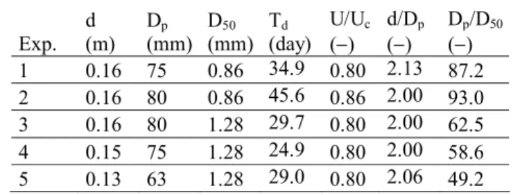
The values of the most important independent va-riables characterizing the experiments are summa-rized in Table 1. The study was made for reasona-bly high flow depth, d = 0.13 m, 0.15 m and 0.16 m. The approach flow velocity, U, was selected to be 80% or 86% (cf. Table 1) of the sand entrain-ment velocity (beginning of motion), Uc. This
va-riable was calculated through the equation sug-gested by Neil (Uc2/(ΔgD50) = 2.5(d/D50)0.2); Δ =
ρs/ρ – 1; ρ = water density; g = acceleration of
gravity. For Exp. #1 (for example), where d = 0.16 m and D50 = 0.86 mm, Uc, U and the flow
discharge, Q, were, respectively, 0.314 ms−1,
0.252 ms−1 and 0.034 m3s−1. The aspect ratio was
such that B/d ≥ 5.2 (B = flume width) and the con-traction ratio was B/Dp ≥ 10.4. These values
indi-cate that wall effect and contraction effect are negligible. Since D50 > 0.8 mm and ρs = 2650
kgm−3 viscous effects can be expected to be small, according to Kothyari et al. (2007). Tests lasted 24.9 days ≤ Td ≤ 45.6 days (Td = test duration),
i.e., much longer than common experiments. The relative flow depth, d/Dp was kept reasonably
constant and ≈2, rendering the effect of this para-meter on the equilibrium scour depth negligibly small; relative sediment size, Dp/D50, varied in the
range 49.2 ≤ Dp/D50 ≤ 93.0, which maximizes the
scour depth.
Table 1. Characteristic variables of the experiments
Exp. d (m) Dp (mm) D50 (mm) Td (day) U/Uc (−) d/Dp (−) Dp/D50 (−) 1 0.16 75 0.86 34.9 0.80 2.13 87.2 2 0.16 80 0.86 45.6 0.86 2.00 93.0 3 0.16 80 1.28 29.7 0.80 2.00 62.5 4 0.15 75 1.28 24.9 0.80 2.00 58.6 5 0.13 63 1.28 29.0 0.80 2.06 49.2
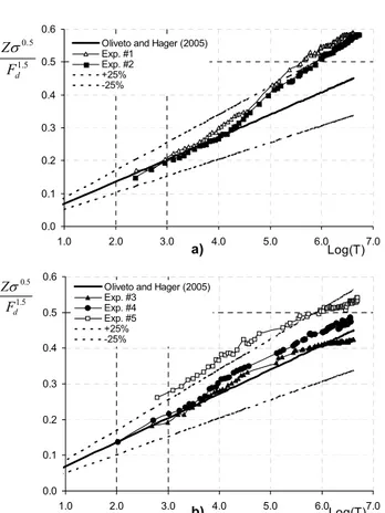
The time records of the scour depth are available at http://w3.ualg.pt/~rlanca/riverflow2010.htm; they are plotted in Fig. 1 as ds vs t (log scale); they
are also given in Fig. 2 by exploiting the coordi-nates suggested by Oliveto and Hager (2002; 2005), i.e.
(
2)
1/3 s R p R d Z z dD z = ∴ = (3) and R t t T = ∴(
)
1/2 50 3 / 1 gD z t R R Δ = σ (4)Fig. 2 also includes the predictor of time evolution of scour depth proposed by Oliveto and Hager (2005):
1/2 3/2
0.068 D d log
Z = Nσ − F T (5)
where Fd = U/(ΔgD50)1/2 is the densimetric Froude
number and N = 1 is a shape factor. Fd was
practi-cally equal for the experiments with a given sand and was taken as the corresponding sand-average for purposes of plotting equation (5).
The inspection of Fig. 1 indicates that equilib-rium was never clearly reached. This is more evi-dent for Exp. #1 and Exp. #2, run for the finer sand. In the case of Exp. #1, two dotted horizontal segments are included, corresponding to horizon-tal plateaux where equilibrium could, a priori, be claimed to have been reached, according to Car-doso and Bettess (1999). Similar plateaux appear
in the other experiments, rendering it clear that the criticism of Radice et al. (2002) is pertinent.
0.020 0.040 0.060 0.080 0.100 0.120 0.140 0.160 0.180 0.200 0.0 0.1 1.0 10.0 100.0 1000.0 ds(m) t (hour) Exp. #1 Exp. #2 Exp. #3 Exp. #4 Exp. #5
Figure 1. Time evolution of the scour depth
0.0 0.1 0.2 0.3 0.4 0.5 0.6 1.0 2.0 3.0 4.0 5.0 6.0 7.0 Log(T) Oliveto and Hager (2005)
Exp. #1 Exp. #2 +25% -25% a) 5 . 1 5 . 0 d F Zσ 0.0 0.1 0.2 0.3 0.4 0.5 0.6 1.0 2.0 3.0 4.0 5.0 6.0Log(T)7.0
Oliveto and Hager (2005) Exp. #3 Exp. #4 Exp. #5 +25% -25% b) 5 . 1 5 . 0 d F Zσ
Figure 2. Time evolution of scour depth written in the coor-dinates of Oliveto and Hager (2005)
The analysis of Fig. 2 reveals that, with the excep-tion of Exp. #5, i) the predictor of Oliveto and Hager (2005) fits the data perfectly, for T < 104, ii) the slope of the observed scour depth evolution is steeper than the slope of the predictor for the finer sand when T > 104, iii) a tendency to equilib-rium is identifiable in the case of the coarser sand (see Exp. # 3 and Exp. #5); iv) the 25% band around the predictor does not really accommodate measurements of Exp. #1(for T > 105) and Exp.
#5.
The time records of scour depth were finally exploited within the framework of Kothyari´s et al. (2007) predictor of scour-depth time evolution. It was concluded that this predictor does not
per-form better than the predictor of Oliveto and Hager (2005) since most of the experimental data fall outside the 25% band; the predictor of Kothyari et al. (2007) largely under-predicts scour depth in four of the five cases.
Although equilibrium was not unambiguously reached, it seems reasonable to postulate that equilibrium must exist since, in nature, there are abutment-like structures where the flow kept run-ning since ever while the scour depth did not in-crease to infinite. Yet, one has to recognize that i) the probability of occurrence of a sufficiently strong turbulent event capable of entraining bed grains will never be null; ii) this probability de-creases as scour progresses, tending asymptoti-cally to zero. Consequently, i) the scour depth will tend to equilibrium but ii) the time required for equilibrium may be rather large, idealized as infi-nite. This is the concept behind equation (1) sug-gested by Bertoldi and Jones (1998) to be fitted to finite-time records of scour and derive the equilib-rium (end) scour depth, for t = ∞.
Thus, equation (1) was fitted to the five data sets. Fig. 3.a) shows the result of this procedure as applied to Exp. #2. Two extents of the record were used in the fitting process: 25 days and the full record. It becomes clear that i) the fitted curves do not perfectly adhere to the scour data, particularly for large values of t; ii) deviations are more pronounced when the fitting process is ap-plied to the shorter duration.
0.040 0.060 0.080 0.100 0.120 0.140 0.160 0.180 0.200 0 200 400 600 800 1000 t (hour) ds (m) data Equation 1 (46 days) Equation 1 (25 days) a) 0.040 0.060 0.080 0.100 0.120 0.140 0.160 0.180 0.200 0 200 400 600 800 1000 t (hour) ds (m) data Equation 2 (46 days) Equation 2 (25 days) b)
Figure 3. a) Data of Exp. # 2 adjusted by equation (1); b) idem for equation (2)
The trend shown in Fig. 3.a) was also observed for the other four experiments although it was less pronounced, particularly for experiments corre-sponding to the coarser sand. The identification of
such trend led to the consideration of equation (2) in the analysis. From Fig. 3.b) it is obvious that this equation fits the data much closer. For this reason, equation (2) was used to derive the end scour of each experiment. It must be stressed that i) the calculations inherently carry unknown er-rors, ii) the errors decrease as the lengths of the scour records used in the fitting procedure in-crease.
Since Exp. #2 was the longer one, it was used to check the order of magnitude of deviations of end scour depth calculated from different-length experiments. For this purpose, the time record was truncated at three different durations, tr < Td.
Equation (2) was applied to the four issued re-cords and the deviations were evaluated assuming that the true end scour is obtained from the ex-trapolation of the entire record (≈46 days) to infi-nite. The output deviations were –4.2% for tr = 25
days, –2.5% for tr = 30 days and –1.2% for tr = 35
days. It can be assumed that, for the remaining (shorter) experiments, deviations associated to the extrapolation of equation (2) to t = ∞ will be of the same order of magnitude or smaller. Smaller deviations are expectable, namely, for Exp(s). #3, #4 and #5, which seem to have attained scour depths closer to equilibrium (cf. Fig. 2.b).
The end scour values, dse, calculated by fitting
equation (2) to the complete scour depth records are given in Table 2. It should be retained here that the determination coefficients of the fitting process were always higher than 0.99. These val-ues of dse are compared with those obtained by
applying the procedures of Melville and Chiew (1999), Cardoso and Bettess (1999) and Grimaldi (2005) to assess equilibrium in laboratory condi-tions.
Table 2. Comparison of time to equilibrium and end scour depth obtained from scour measurements through different approaches
dse
(m) M. & C. (1999) C. & B. (1999) G. (2005) Exp.
(Eq. 2) tM
(day) d(m) se Δd(%) se t(day)C (m) dse Δd(%) se t(day) G d(m) se Δd(%) se # 1 0.173 3.1 0.139 -19 12.4 0.159 -8 6.1 0.150 -13
# 2 0.210 5.1 0.161 -23 19.4 0.182 -13 10.0 0.174 -17
# 3 0.130 3.1 0.121 -7 4.5 0.127 -2 3.1 0.121 -7
# 4 0.140 4.2 0.124 -11 8.2 0.132 -6 6.9 0.126 -10
# 5 0.128 3.1 0.118 -8 6.3 0.124 -3 5.0 0.118 -8
M. & C. (1999) = Melville and Chiew (1999); C. & B. (1999) = Cardoso and Bettess (1999); G. (2005) = Grimaldi (2005).
According to the criterion of Melville and Chiew (1999) – which coincides with the criterion of Coleman et al (2003) in the present situation –, equilibrium should have been obtained at time tM
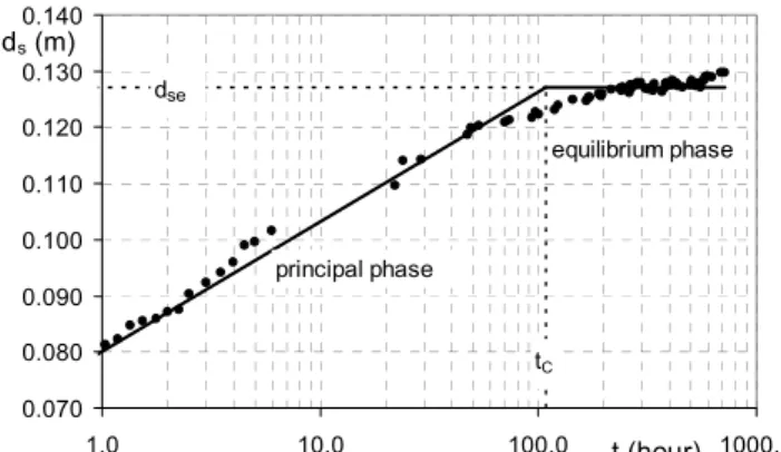
(cf. Table 2). The criterion of Cardoso and Bettess (1999), illustrated in Fig. 4, for Exp. # 3, leads to the values of time to equilibrium, tC, included in
the same table; the equilibrium time associated with the criterion of Grimaldi (2005) is tG. The
criterion of Cardoso and Bettess (1999) was ap-plied to the last plateau of each scour record.
The inspection of Table 2 leads to conclude that: i) in general, tC > tG ≥ tM; ii) the three
meth-ods lead to the experimental under-estimation of the equilibrium scour depth; iii) as expectable from the values of tC, the smaller deviations on dse
are those issued by the method of Cardoso and Bettess (1999); iv) the stronger deviations oc-curred for the finer sand (Exp. #1 and #2) irre-spective of the method; v) deviations range from – 2% (for tC, Exp. #3) to –23% (for tM, Exp. #2).
Conclusion iv) might derive from the fact that, since the sand is finer, the intensity of the vortical system – which can be expected to be similar in the five experiments as Dp, d and U did not
change much – remains strong enough to entrain the bed sediment for longer time, leading to higher durations before equilibrium is reached.
0.070 0.080 0.090 0.100 0.110 0.120 0.130 0.140 1.0 10.0 100.0 t (hour) 1000.0 ds (m) principal phase equilibrium phase dse tC
Figure 4. a) Definition of time to equilibrium and end-scour depth according to Cardoso and Bettess (1999)
The values of Table 2 should still be added with those of the deviations inherent to the use of the 6-parameters polynomial function, equation (2). These deviations where seen to be –1% to –4%. In practice, this means that the use of common meth-ods to estimate pier end-scour depth from labora-tory tests can lead to under-estimations of up to ≈30%, depending on the method. In contrast, the methods of Cardoso and Bettess (1999) and Ber-toldi and Jones (1998) were verified to be practi-cally equivalent for assessing equilibrium scour at abutments by Fael et al. (2006).
The literature on local scour includes some predictors of time to equilibrium. The predictor of Franzetti et al. (1994) was already presented in Section 2, while for d/Dp ≈ 2.0 the predictor of
Melville and Chiew (1999) reads
0.25 30.89 p 0.4 M c p D U d t U U D ⎛ ⎞ ⎛ ⎞ = ⎜ − ⎟⎜⎜ ⎟⎟ ⎝ ⎠⎝ ⎠ (6)
with tM expressed in days; the predictor of time to
equilibrium suggested by Kothyari et al. (2007) is
1 5
log = 4.8T F (7)d
where T and Fd keep the same meaning as in
equations (4) and (5).
The values of time to equilibrium issued from these three predictors are presented in Table 3, where the subscript F stands for Franzetti et al. (1994) and the subscript K stands for Kothyari et al. (2007). The table also includes the equilibrium scour depths observed at time to equilibrium and the percent deviations towards the equilibrium scour depth calculated through equation (2) as ex-trapolated to t = ∞. The values of tM are, with no
surprise, similar to those presented in Table 2; tF >
tM ≈ tK in all cases. The values of percent
devia-tion on the estimated equilibrium scour depth are significant and vary between –4% and –24%.
The previous discussion profusely shows that common methods used in practice to decide on whether a given scour experiment has reached the equilibrium phase or not may be erroneous. It also shows that known predictors of time to equili-brium may imply significantly wrong predictions of equilibrium depth.
Table 3. Comparison of time to equilibrium and end scour depth obtained from existing predictors.
Exp. dse (m) F. (1994) M. & C. (1999) K. (2007) (Eq. 2) tF (day) dse (m) Δdse (%) tM (day) dse (m) Δdse (%) tK (day) dse (m) Δdse (%) # 1 0.173 6.3 0.150 -13 4.1 0.145 -16 4.0 0.145 -16 # 2 0.210 6.2 0.161 -23 4.5 0.160 -24 5.2 0.165 -22 # 3 0.130 5.4 0.124 -4 3.4 0.121 -7 3.6 0.122 -6 # 4 0.140 5.1 0.125 -11 3.2 0.121 -14 3.4 0.125 -11 # 5 0.128 4.3 0.118 -8 2.8 0.117 -9 2.8 0.116 -9 F. (1994) = Franzetti et al. (1994); M. & C. (1999) = Melville and Chiew (1999); K. (2007) = Kothyari et al. (2007).
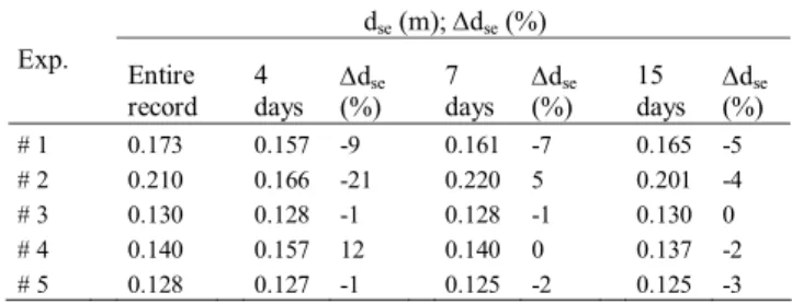
So, the following question is raised: how long should last experiments on local scour at single cylindrical piers to assure sufficiently precise pre-dictions of equilibrium depth? Assuming equili-brium to occur at t = ∞, equation (2) was syste-matically applied to three partitions of each scour record defined at t = 4, 7 and 15 days. It is worth to note that the determination coefficient was in all cases > 0.99. The outputs of this procedure are compared in Table 4 with those obtained from the entire records.
Table 4 indicates that i) the 6-parameters poly-nomial extrapolations on the basis of 4 days-long experiments are not satisfactory; ii) reasonable ex-trapolations are expectable from ≈ 7 days-long re-cords; iii) only marginal improvements may be expected from experiments lasting longer than 7 days.
Table 4. Equilibrium scour depth obtained by adjusting and extrapolating equation (2) to scour records of different dura-tions.
dse (m); Δdse (%) Exp.
Entire
record 4 days Δd(%) se days 7 Δd(%) se 15 days Δd(%) se
# 1 0.173 0.157 -9 0.161 -7 0.165 -5 # 2 0.210 0.166 -21 0.220 5 0.201 -4 # 3 0.130 0.128 -1 0.128 -1 0.130 0 # 4 0.140 0.157 12 0.140 0 0.137 -2 # 5 0.128 0.127 -1 0.125 -2 0.125 -3 5 CONCLUSIONS
From the previous discussion, the following im-portant conclusions can be drawn:
i) Scour experiments at single cylindrical piers, run for up to ≈46 days, did not unambiguously reach equilibrium, with special emphasis in the tests with the finer sand.
ii) Common methods used in practice to decide on the initiation of the equilibrium phase may be rather erroneous.
iii) Known predictors of time to equilibrium may lead to significantly wrong predictions of equilibrium scour depth.
iv) Typically 7 days long scour-depth records adjusted though equation (2) and extrapolated to infinite time seem to render robust vales of the equilibrium scour depth at single cylindrical piers.
ACKNOWLEDGEMENTS
The authors wish to acknowledge the financial support of the Portuguese Foundation for Science and Technology through the PhD grant SFRH/BD/49296/2008 and the research project PTDC/ECM/101353/2008.
REFERENCES
Bertoldi, D.A., Jones, J.S. 1998. Time to scour experiments as an indirect measure of stream power around bridge piers. Proceedings of the International Water Resource Engineering Conference, Memphis, Tennessee, August 1998, pp. 264-269.
Cardoso, A.H., Bettess, R. 1999. Effects of time and chan-nel geometry on scour at bridge abutments. ASCE Jour-nal of Hydraulic Engineering, Vol. 125 nº 4 , Abril. Chabert, J., Engeldinger, P. 1956. Etude des affouillements
autour des piles des ponts. Laboratoire National d’Hydraulique, Chatou, France.
Coleman, S.E., Lauchlan, C.S., Melville, B.W. 2003. Clear-water scour development at bridge abutment. Journal of Hydraulic Research, IAHR, vol. 41, nº 5, pp. 521–531. Ettema, R., 1980. Scour at bridge piers. University of
Auck-land, School of Engineering, AuckAuck-land, New ZeaAuck-land, Rep. No. 216.
Fael, C.M.S., G. Simarro-Grande, Martín-Vide J.P., Cardoso, A.H. 2006. Local scour at vertical-wall abut-ments under-clear water flow conditions. Water Re-sources Research. vol. nº 42, W10408.
Franzetti, S., Larcan; E., and Mignosa, P. 1982. Influence of tests duration on the evaluation of ultimate scour around circular piers, International Conference on the Hydraulic Modelling of Civil Engineering Structures, paper G2, Coventry, England.
Franzetti, S., Malavasi, S., and Piccinin, C. 1994. Sull’erosione alla base delle pile di ponte in acque chiare. Proc., XXIV Convegno di Idraulica e Costruzioni Idrauliche, Vol. II, T4 13–24 (in Italian).
Grimaldi, C. 2005. Non-conventional countermeasures against local scouring at bridge piers. Ph.D. thesis, Hy-draulic Engineering for Environment and Territory, Univ. of Calabria, Cosenza, Italy.
Hoffmans, G.J.C.M., Verheij, H.J. 1997. Scour manual. A.A. Balkema, Rotterdam, p. 205.
Kothyari, U. C., Hager, W. H., Oliveto, G. 2007. General-ized approach for clear-water scour at bridge founda-tions elements. ASCE Journal of Hydraulic Engineering, Vol. 133(11), pp 1229-1240.
Laursen, E.M. 1963. An analysis of relief bridge scour. Journal of Hydraulics Division, ASCE, Vol. 89, No. HY3, pp. 93-118.
Melville, B. W., Chiew Y.M. 1999. Time scale for local scour at bridge piers, Journal of Hydraulic Engineering, Vol.125, Nº1, 59–65.
Oliveto, G., Hager, W. H. 2002. Temporal evolution of clear-water pier and abutment scour. ASCE Journal of Hydraulic Engineering, Vol. 128 nº 9, Sep.
Oliveto, G., Hager, W. H. 2005. Further results to time-dependent local scour at bridge elements. ASCE Journal of Hydraulic Engineering, Vol. 131(2), pp 97-105. Radice, A., Franzetti, S., Balio, F. 2002. Local scour at
bridge abutments. River Flow 2002, Bousmar & Zech (eds.), Balkema Publishers, The Netherlands, 1059– 1068.