Revista da Universidade Vale do Rio Verde ISSN: 1517-0276 / EISSN: 2236-5362
Vol. 17 | n. 2 | Ano 2019
Leda Grasiele Oliveira [email protected] Lincoln Frias [email protected] Patrícia de Siqueira Ramos [email protected]
THE VALUE OF HIGH SCHOOL:
THE IMPACT OF SCHOOLING
ON INCOME AND LABOR
MARKET INSERTION
_______________________________________________
ABSTRACT
There is some consensus that school education is central for the socioeconomic development of a country. Thus, the purpose of this paper is to evaluate the effect of secondary education on labor market insertion, analyzing the income and the different types of occupation of individuals with secondary education and those with only elementary education. In addition to a descriptive analysis, the paper employs multiple regression to understand the relationship between the level of education and the average income, evaluating the effect of secondary education using other variables as controls (e.g., such as sex and age). The data comes from the Continuous Household National Sample Survey (Pesquisa Nacional por Amostra de Domicílios Contínua - PNADC), second quarter of 2017, and the analysis was done in the Python programming language. Individuals with secondary education tend to have higher incomes than those with only elementary education (the additional amount varying between R$206 and R$391 according to different models). In addition, the effect of secondary education varies by age and sex, with women tending to have lower incomes than men.
Keywords: Education. High school. Labor Market.
Income. Brazil.
O VALOR DO ENSINO MÉDIO:
O IMPACTO DA ESCOLARIDADE
SOBRE OS RENDIMENTOS E A
INSERÇÃO NO MERCADO DE
TRABALHO
____________________________________________ RESUMOExiste certo consenso de que a educação escolar é fundamental para o desenvolvimento socioeconômico de um país. Sendo assim, o objetivo da presente pesquisa é avaliar o efeito do ensino médio sobre a inserção no mercado de trabalho, analisando os rendimentos e os diferentes tipos de ocupação de indivíduos que possuem o ensino médio e daqueles que possuem apenas o ensino fundamental. Além de uma análise descritiva, utilizou-se como metodologia a análise de regressão múltipla, com o intuito de entender a relação entre o nível de instrução e o
e utilizando outras variáveis como controle (sexo e idade, por exemplo). Os dados são referentes ao segundo trimestre de 2017 da Pesquisa Nacional por Amostra de Domicílios Contínua (PNADC) e foram analisados usando a linguagem de programação Python. Os indivíduos que possuem o ensino médio tendem a ter rendimentos maiores do que aqueles que possuem apenas o ensino fundamental (essa diferença varia de R$206 a R$391 reais de acordo com o modelo utilizado). Além disso, observa-se que o efeito do ensino médio varia para diferentes idades e para cada um dos sexos, com as mulheres tendendo a possuir rendimentos menores do que os homens.
Palavras-chave: Educação. Ensino médio. Mercado de
trabalho. Rendimento. Brasil.
1. INTRODUCTION
There is a widespread consensus that school education is an essential requirement of economic development. For example, political candidates of diverse lineages usually demand investment in this area.
The assumption is that education has monetary and non-monetary effects. Regarding the first, education would be able to develop skills that will be valued by the labor market, resulting in monetary gains. On the other hand, education would also bring non-monetary returns in terms of political participation, better decisions about health and child care, as well as other decisions important in the long run (OREOPOULOS; SALVANES, 2011).
Therefore, this paper evaluates the effect of high school on labor market insertion, contrasting individuals with high school and those limited to elementary school in relation to their income and types of jobs. In addition to descriptive statistics, a regression analysis is done to understand the relationship between the level of
education and income. The main hypothesis of this paper is that different levels of education may be related to different labor conditions.
The article is divided into four sections, in addition to this introduction. The next one surveys the literature on the relation between education and labor market. The third section presents information about the data and the statistical methods employed in the analysis whereas the fourth section contains their results. The last section presents the final remarks.
2. EDUCATION AND THE LABOR MARKET
Much of the inequality in labor earnings is due to schooling differences among workers. In this respect, the labor market translates educational inequality into income inequality. However, the inequality revealed by the labor market is not determined only by the magnitude of educational inequality among workers. It also depends on how the market values these differences in schooling (BARROS; FRANCO; MENDONÇA, 2007).
Beside this, education is related not only to income, but also to probability of getting a job. In 2002, in Brazil, an individual with incomplete high school had 18% chance of being unemployed. However, after completing high school, the chances of unemployment fell to 11% (TAFNER, 2006). Oreopoulos and Salvanes (2011) present results in the same direction, with less educated individuals being more likely to be unemployed.
The “sheepskin effect” is a decisive phenomenon in this context. It means that an additional year of schooling has a greater effect
on income when it corresponds to the conclusion of a cycle, that is, the acquiring of a diploma.The diploma is considered a kind of signal for the labor market, where the fact that the individual has a diploma indicates that he has the potential to perform certain activities(COELHO; CORSEUIL, 2002).
This effect can be observed for all cycles, in lower elementary school, upper elementary school, high school and college. In Brazil the rates of return per educational cycle are quite high, especially for the secondary and higher education (BARBOSA-FILHO; PESSÔA, 2008).
Several authors calculate the monetary returns of education, with results varying according to region, sex and race. Crespo and Reis (2009) pointed to a reduction of sheepskin effect in recent years, meaning that the completion of a degree is losing value over time. However, the higher effects for advanced levels remain. While in 1982, lower elementary school increased income by 12%, in the 90s, completing this cycle was no longer significant. High school had an effect of 32% in 1982 and fell to 27% in 2004.
There are also regional differences in the monetary effects of education. Suliano and Siqueira (2012) investigated these differences by comparing the Northeast and Southeast regions of Brazil. The results pointed to a higher effect of schooling in the Southeast region. In the Northeast region, an additional year of education would raise income by up to 16%, whereas in the Southeast region it would raise salaries by up to 13%.
3. METHODS
This paper uses descriptive and regression analysis in order to understand the relationship between the level of education and the average income. The analysis were performed in the Python programming language and the codes are available at GitHub (github.com/*******).
The data refer to the second quarter of 2017 and were taken from the Continuous National Household Sample Survey (Pesquisa Nacional por Amostra de Domicílios - PNADC). Some restrictions were applied to the data set. The first one refers to age, where individuals younger than 17 years were withdrawn in order to include only those who already had the chance to complete high school. Then, those who was still attending school were removed, remaining only those who are no longer studying. A third restriction refers to schooling, including only those with elementary and high school. Finally, two versions of the resulting data set were analyzed: one containing only those individuals who have some income and another with all the individuals, that is, including those with no income.
Regression analysis investigate the association among two or more variables (WOOLDRIDGE, 2014). It can be employed to give two different kinds of answers: structural or causal (ANGRIST; PISCHKE, 2017). In the first case, the models use a large amount of explanatory variables without privileging any of them in order to explain all the variation of a certain phenomenon. The main purpose is to explain as much as possible the variation of the dependent variable (which is measured by R²). In
the second style of regression analysis, much influenced by randomized controlled experimental studies, relatively few variables are included in the model, making a clear distinction between what is the variable of interest and what are the control variables. That is, these are included in the model only to isolate the effect of the variable of interest from which the causal effect is estimated. The central aim in this case is to analyze the changes in the coefficient of the variable of interest arising from the inclusion of control variables and from different restrictions of the sample. The present study uses regression analysis in this second sense.
4. RESULTS
In 2017, Brazil still had very low levels of education. A third of the population had only
incomplete elementary school (33.9%). Another
third was limited to a high school diploma (29.6%). The remaining third was divided between those with a elementary school diploma (13.6%), the uneducated (11.3%) and those with higher education (11.6%).
Viewed from another perspective, 58.8% of population (those uneducated, with incomplete elementary school and with elementary school) did not even complete high school, that is, most of the population was restricted to the elementary school.
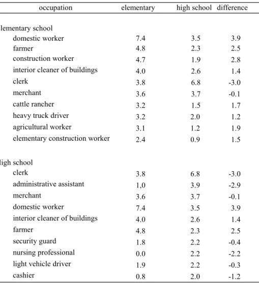
In order to familiarize the reader with the distribution of the most common occupations in Brazil, Table 1 shows the ten occupations with the highest percentages of workers, comparing those with only elementary education with those who completed high school. In the first portion of the
table are the ten most common occupations among individuals who completed elementary education, whereas in the second portion are the ten most common occupations of individuals who have completed high school.
Most workers with elementary education are in positions who tend to be more informal, such as domestic worker (7.4%), farmer (4.8%) and construction worker (4.7%), for example. For workers with high school, the situation is not very different, but there are divergences. Of these, most are working as clerk (6.8%), followed by administrative assistants (3.9%) and merchants (3.7%).
While the three most common occupations of those with primary education are domestic worker, farmer and construction worker, among those with high school, domestic worker is in the fourth position; farmer is in sixth position; and construction worker does not even appear among the ten most common occupations. In addition, the occupations of cattle rancher, heavy truck driver, agricultural worker and construction worker, which are among the most common for those with elementary school, do not appear among those with high school. On the other hand, administrative assistant, security guard, nursing professional, light vehicle driver (car, taxi, pickup truck) and cashier are occupations that are among the most common among those with high school, but not in the case of those limited to elementary school.
Table 1 – Main occupations by educational level (%)
occupation elementary high school difference Elementary school
domestic worker 7.4 3.5 3.9
farmer 4.8 2.3 2.5
construction worker 4.7 1.9 2.8 interior cleaner of buildings 4.0 2.6 1.4
clerk 3.8 6.8 -3.0
merchant 3.6 3.7 -0.1
cattle rancher 3.2 1.5 1.7 heavy truck driver 3.2 2.0 1.2 agricultural worker 3.1 1.2 1.9 elementary construction worker 2.4 0.9 1.5 High school
clerk 3.8 6.8 -3.0
administrative assistant 1,0 3.9 -2.9
merchant 3.6 3.7 -0.1
domestic worker 7.4 3.5 3.9 interior cleaner of buildings 4.0 2.6 1.4
farmer 4.8 2.3 2.5
security guard 1.8 2.2 -0.4 nursing professional 0.0 2.2 -2.2 light vehicle driver 1.9 2.2 -0.3
cashier 0.8 2.0 -1.2
Source: Own elaboration. Data source: PNADC (2017). Observation: only 17 years or old who do not attend school.
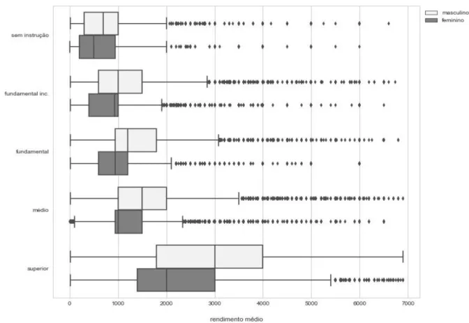
Figure 1 shows the average income according to sex and educational level. Income values was restricted to an upper limit of R$7,000 to make it easier to see and interpret the plot. This number was reached removing the top 1% income among those with elementary and high school, that is, taking away the last percentile of income distribution.
At first sight, what can be observed is that the average income has a tendency to increase with schooling. The average income of uneducated people is very low, around R$700 for males and R$500 for females. The average income of those with incomplete elementary
school is a little higher and so on. In addition, it is possible to observe that for all educational levels women have lower income than men.
Despite the fact that in recent years women have higher levels of education, women’s earnings are still lower than those of men. Other authors found similar results (MONTEIRO; DIAS; DIAS, 2011; SILVEIRA et al., 2015; COELHO; CORSEUIL, 2002, DALCIN; ZANON, 2017). In studies that calculate the internal rate of return for schooling, when the rate is disaggregate by sex, the return is lower for women. For example, the internal rate of return found by Monteiro, Dias and Dias (2011) was 11.8%, but when calculated
for each sex, the values diverged, being 19.8% for males and 16.1% for females.
Figure 1 – Income by sex and educational level
Source: Own elaboration. Data source: PNADC (2017). Observation: only 17 years or old who do not attend school and with income below R$7,000.
In this same perspective, Silveira et al. (2015), using the 2009 PNAD data, also found different returns for men and women, with 11.1% for men and 9.9% for women, with rates varying among the different regions of Brazil, but being lower for women in all cases. Dalcin and Zanon (2017) calculated the internal rate of return for Rio Grande do Sul using the PNADs of 2002 to 2014 and also found a smaller return for women.
The purpose of regression analysis in this paper is to understand the effect of high school on income. Thus, the dependent variable is the income of people over 17 years old who do not
or high school. The variable of interest is the level of education, limited to those two levels. Other variables are used as control - such as sex, age, state and type of area (state capital, metropolitan area and rest of the state) - in order to understand if the effect of high school is different for individuals with different characteristics.
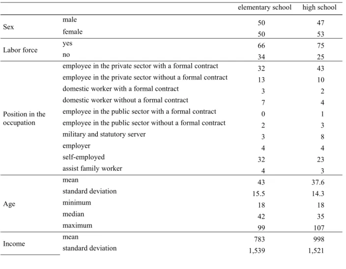
Table 2 presents a statistical summary of the variables included in the models. Among individuals with elementary school, there is an equal division among the sexes. For individuals with high school, 53% are women and 47% are men. Among those with elementary school, 66%
for a job. In the case of individuals with high school, the portion is higher, 75%.
Concerning the position in the occupation of those with elementary school, the majority is employed in the private sector with formal contracts (32%) or self-employed (also 32%). Among those with high school, most are also employed in the private sector with a formal contract (43%), 11 percentage points higher than their elementary school counterparts. In the second place are also self-employed workers (23%), again with a difference of 9 percentage points compared to those with elementary school.
Another difference is that the percentage of people working as military and statutory servants is higher among those with high school (8% against 3%). The percentage of domestic
workers without a formal contract is higher among those with elementary education compared to those with high school (7% and 4% respectively).
Regarding age, among individuals with elementary school, the average is 43 years old and the median is 42 years old. The group with high school is younger, with a mean difference of around 7 years.
The average income of the group with elementary school is R$783, whereas in the case of people with high school diplomas it is R$998, a difference of R$215. Looking at the median, the difference is even greater, with those with high school having an income twice as high than those with elementary school (R$937 and R$450, respectively).
Table 2 – Descriptive analysis (including individuals without income)
elementary school high school
Sex malefemale 50 47
50 53
Labor force yesno 66 75
34 25
Position in the occupation
employee in the private sector with a formal contract 32 43 employee in the private sector without a formal contract 13 10 domestic worker with a formal contract 3 2 domestic worker without a formal contract 7 4 employee in the public sector with a formal contract 0 1 employee in the public sector without a formal contract 2 3 military and statutory server 3 8
employer 4 4
self-employed 32 23
assist family worker 4 3
Age mean 43 37.6 standard deviation 15.5 14.3 minimum 18 18 median 42 35 maximum 99 107
Income meanstandard deviation 783 998 1,539 1,521
minimum 0 0
median 450 937
maximum 166,666 100,000
Data source: PNADC (2017). Observation: only 17 years or old who do not attend school.
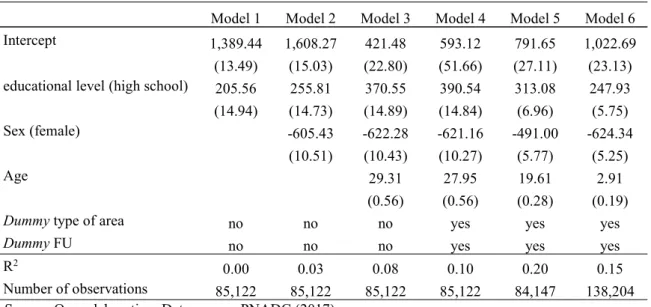
Table 3 presents the results of the six regressions models. In the first five models the data refer only to those with some income. However, in the fifth model, it includes only those with incomes lower than R$7,000. The sixth model included only those with incomes lower than R$7,000, but individuals without income were now included. Table 3 shows the R² (coefficient of determination) of the models, denoting how much each of them can explain the variation in the explained variable (income). The model 5 has the highest explanatory power, explaining 20% of the variation of income. The values in parenthesis are the standard errors of each explanatory variable.
In the model 1 no variable was used as control, the level of education being the only explanatory variable. Thus, the model presents only the effect of high school on income (mixing with the effect of the omitted variables). Since the level of education is a categorical variable composed of two categories (elementary and high school), the model uses one of the categories as a base. In this case the category used as a base was the elementary school. Thus, the intercept (1,389.4) is the average income of a individual with only elementary school. The coefficient of the educational level (205.6) is the effect of high school on income. That is, according to this model, the fact that the individual has completed high school means that he has an income, on average, R$205.6 higher than those with only elementary school.
In the model 2, the variable sex was added as a control variable, in order to understand if the effect of high school on income will be different for both sexes. It can be seen that by adding this variable, both the intercept and the coefficient of the educational level have different values, which confirms that by controlling for sex, the effect of high school on income is different. The variable sex, as well as the level of education, is categorical and, in this case, the male category was taken as the basis. In this model the intercept has a value of 1,608.3, which means that if the individual has only elementary school and he is male, in average, his income will be R$1,608.3. The value of the coefficient of the educational level is 255.8, which means that if the individual has high school, his income tends to increase by an average of R$255.8. On the other hand, the negative coefficient for the variable sex in the amount of -605.43 means that if the individual is female, her income tends to be on average R$605.4 lower.
The model 3 expanded the previous model including age as a control variable. Again, both the intercept and the coefficient changed. The intercept in this model is smaller, 421.5. The coefficient of the educational level is higher (370.5), indicating that the effect of high school is higher than in the previous models. The coefficient of the variable sex, in turn, is -622.3. On the other hand, the coefficient of the variable age was 29.3, which means that an additional year of age increases income by R$29.3, on average.
Thus, controlling for age and sex, the coefficient of the educational level is higher, indicating that their effect on income was confounded with the effect of education in the first model, when they were omitted.
In the fourth model two dummy variables were included, state and type of area. Again the effect of high school on income increases, since the coefficient of the educational level has increased to 390.5, which means that there is a different effect of high school in different locations.
In the fifth model the same variables of the previous one were used (educational level, sex, age, type of area and state), but, as previously mentioned, the data are restricted to individuals with income lower than R$7,000. As a result, the
effect of the educational level decreases compared to the previous model. The effect of sex also decreases with the coefficient, lowering from -621.2 to -491. In addition, the effect of age also diminishes, suggesting that these variables have less influence on the lower incomes.
Finally, the model 6 includes the same variables and again includes only those with incomes lower than R$7,000, but now individuals without income were also included. The effect of high school decreased compared to the previous model, because individuals without income were considered. The same happened with the effect of sex, which is also greater in this model, since a considerable portion of people without income is female. On the other hand, the effect of age has a great reduction from 19.6 to 2.9.
Table 3 – Results of the regression models
Model 1 Model 2 Model 3 Model 4 Model 5 Model 6 Intercept 1,389.44 1,608.27 421.48 593.12 791.65 1,022.69 (13.49) (15.03) (22.80) (51.66) (27.11) (23.13) educational level (high school) 205.56 255.81 370.55 390.54 313.08 247.93 (14.94) (14.73) (14.89) (14.84) (6.96) (5.75) Sex (female) -605.43 -622.28 -621.16 -491.00 -624.34
(10.51) (10.43) (10.27) (5.77) (5.25)
Age 29.31 27.95 19.61 2.91
(0.56) (0.56) (0.28) (0.19)
Dummy type of area no no no yes yes yes
Dummy FU no no no yes yes yes
R2 0.00 0.03 0.08 0.10 0.20 0.15
Number of observations 85,122 85,122 85,122 85,122 84,147 138,204 Source: Own elaboration. Data source: PNADC (2017).
This set of models shows that high school provides higher monetary returns when compared to elementary school, which agrees with the results presented by Monteiro, Dias and Dias (2011), that found a lower return rate for elementary school compared to high school. Coradini (2014) agrees that the positive relations between the years of school and the amount of income were more significant for the higher educational levels.
In addition, when analyzing the most common jobs for the two educational levels, it was observed that among those with elementary school they tend to be more informal, such as domestic worker, farmer, construction worker, etc. In the case of individuals with high school, the situation is different. For example, the most common occupation is clerk; the second one is administrative assistants; and the third, merchants. That is, these are occupations that are less informal and consequently have better working conditions and higher compensations.
This divergence on the characteristics of the occupations agrees with the results from the regression, according to which workers with high school diplomas are better paid. And this also confirms that the educational level leads to higher incomes not by an increase in productivity in the same jobs, but by giving the opportunity to fill different occupations. That is, the relation between educational level and income is mediated by the type of occupation. Those with higher educational levels are more likely to have occupations that offer higher incomes.
5. FINAL REMARKS
Given the relevance of schooling for individuals and for society as whole, the present paper investigated the effect of high school on income and on the kind of jobs. The analysis showed a significant difference in income according to the educational level of the individuals. In addition, there was also a difference between the the most common occupations of those with only elementary education when compared to those with high school, with the former finding themselves in more informal jobs.
Another contribution of this paper was to quantify the effect of secondary education on income, whose value varied between R$206 and R$391, depending on the variables used as control (such as age, sex, type of area and state). In addition, the analysis confirms that women tend to have lower income than men and that the greater the age, the higher the income. Thus, the regression models identified an effect of high school on earnings and that this effect is not the same for men and women and for different ages. REFERENCES
ANGRIST, J.; PISCHKE, J. Undergraduate econometrics instruction: through our classes, darkly.
Journal of Economic Perspectives, v. 31, n. 2, p.
125-144, 2017.
BARBOSA-FILHO, F. H.; PESSÔA, S. Retorno da educação no Brasil. Pesquisa e Planejamento Econômico, vol. 38, n. 1, 2008.
BARROS, R. P.; FRANCO, S.; MENDONÇA, R. A recente queda da desigualdade de renda e o acelerado progresso educacional brasileiro da última década. Brasília: Ipea. Texto para discussão, n.
1304, 2007.
COELHO, A. M.; CORSEUIL, C. H. Diferenciais salariais no Brasil: um breve panorama. Rio de Janeiro: IPEA, 2002 (Texto para Discussão, n. 898).
CRESPO, A; REIS, M. C. Sheepskin effects and the relationship between earnings and education: analyzing their evolution over time in Brazil.Revista Brasileira de Economia, v. 63, n. 3, p. 209-231, 2009.
CORADINI, O. L. Efeitos da educação formal, categorias ocupacionais e posição social. Sociedade e Estado, v. 29, n. 2, p. 511-538, 2014.
DALCIN, A.; ZANON, D. Taxa interna de retorno da educação: uma análise não paramétrica para o Rio Grande do Sul. Ensaios FEE, v. 38, n. 2, p. 251-272,
2017.
INSTITUTO BRASILEIRO DE GEOGRAFIA E ESTATÍSTICA (IBGE). Pesquisa Nacional por Amostra de Domicílios. Rio de Janeiro: Instituto
Brasileiro de Geografia e Estatística, 2014. Disponível em:
https://ww2.ibge.gov.br/home/estatistica/indicadores/tr abalhoerendimento/pnad_continua/default.shtm. Acesso em: 20 jul. 2018.
MONTEIRO, W. F.; DIAS, J.; DIAS, M. H. A. Taxa de retorno da escolaridade nos estados brasileiros: crescente ou decrescente? In: Anais do XXXVII
Encontro Nacional de Economia.
ANPEC-Associação Nacional dos Centros de Pósgraduação em Economia, 2011.
OREOPOULOS, P.; SALVANES, K. G. Priceless: The nonpecuniary benefits of schooling. Journal of Economic Perspectives, v. 25, n. 1, p. 159-184, 2011.
SILVEIRA, G. F. et al. Retornos da escolaridade no Brasil e regiões.Gestão & Regionalidade, v. 31, n. 91,
2015.
SULIANO, D. C.; SIQUEIRA, M. L. Retornos da educação no Brasil em âmbito regional considerando um ambiente de menor desigualdade. Economia Aplicada, v. 16, n. 1, p. 137-165, 2012.
TAFNER, P. Educação no Brasil: atrasos, conquistas e desafios. In: IPEA. Brasil: o estado de uma nação – mercado de trabalho, emprego e informalidade, Rio
de Janeiro: IPEA, cap. 3, 2006.
WOOLDRIDGE, J. M. Introdução à Econometria:
uma abordagem moderna. São Paulo: Cengage Learning, 2014.