THROUGH AN ECOLOGICAL MODEL By Vânia Sofia de Oliveira Bento

(1)

NEW UNIVERSITY OF LISBON

Faculty of Sciences and Technology

Depart. of Sciences and Environmental Engineering

OYSTERS RETURN TO THE TAGUS ESTUARY

THROUGH AN ECOLOGICAL MODEL

By

Vânia Sofia de Oliveira Bento

Dissertation submitted to the Faculty of Sciences and Technology of

New University of Lisbon for obtaining the degree of Master in

Environmental Management Systems

Adviser: Prof. J. Gomes Ferreira

Lisbon

(2)

(3)

Acknowledgements

The present work would not have been achieved without the collaboration of some people. To whom I want to say thank you:

To my adviser Prof. J. Gomes Ferreira, for this opportunity, for his availability and his teaching which allowed me to carry out this work.

To Dr. Laudemira Ramos, who provided me many bibliographic materials.

To Dr. Teresa Simas, for her time spent.

To Dr. Ana Nobre and Dr. Ana Sequeira of IMAR – Center for Ecological Modelling, who were always available for answering my queries.

(4)

(5)

Abstract

Aquaculture is an activity that has been increasing along the last years. Until the 1970’s Portugal and more specifically the Tagus estuary, was the major exporter of oysters in Europe. Factors like TBT and oysters gill disease had made that the shellfish aquaculture has never been again practised in Tagus estuary. According to that, this work intends to concept and to implement an ecological model that develops the oysters growth in order to them return to the estuary. To begin with, the model was calibrated with data from Database of 1980 and then validated with Database of 1982. The model results have shown a good correlation with measured data, so it was supposed as a good model.

After that, it was simulated two different scenarios. The first one it was increased 30C in water temperature and in the second one it was changed the seeding day to the 90 day instead the 120 day. The results illustrate that in scenario I, the production of oysters decrease as well as the oyster individual weight and length, and in scenario II, however the oyster individual growth as decrease a little the oyster total harvest as increase.

With these approaches, it will be possible to define the better conditions in order to achieve a good model that can be able to optimise the production of oyster in the Tagus estuary.

(6)

(7)

Index

1. Introduction ...1

1.1. Problem definition ...1

1.1.1. Aquaculture worldwide ...1

1.1.2. Aquaculture in Portugal ...2

1.1.3. Aquaculture Legislation ...4

1.1.4. Carrying Capacity...5

1.1.5. Ecological models ...7

1.2. State of art ...8

1.3. Objectives... 13

2. Methodology... 15

2.1. Study area... 15

2.2. Localization of the aquaculture areas and definition in GIS... 16

2.3. Loading and treatment of data... 16

2.3.1. Water quality... 17

2.3.2. Grow and techniques of culture... 18

2.4. Application of ecological model... 20

2.4.1. Calibration ... 24

2.4.1.1. Forcing Functions... 25

2.4.1.2. State Variables... 26

2.4.2. Validation ... 27

2.4.2.1. Forcing Functions... 27

2.4.2.2. State Variables... 27

(8)

3. Results and discussion ...29

3.1. Calibration ...29

3.1.1. Flow...29

3.1.2. Water Temperature...30

3.1.3. Salinity ...34

3.1.4. Suspended Particulate Matter (SPM)...38

3.1.5. Phytoplankton ...43

3.1.6. Zoobenthos ...47

3.2. Validation ...48

3.2.1. Water Temperature...48

3.2.2. Salinity ...51

3.2.3. Suspended Particulate Matter...54

3.2.4. Phytoplankton ...57

3.2.5. Zoobenthos ...60

3.3. Scenario I...61

3.4. Scenario II ...63

4. Conclusion ...65

5. References ...67

Annexes ...73

Annex A – Data of zoobenthos from Esperança (1981, 1982)...73

(9)

Index of figures

Figure 1.1 – Shell deposits in Tagus estuary ... 3

Figure 1.2 – Evolution of Oyster Production in Portugal – Font: INE/DGRA... 4

Figure 1.3 – Image of Crassostrea angulata ... 11

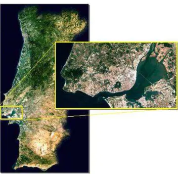
Figure 2.1 – Localization of Tagus estuary in Portugal map... 15

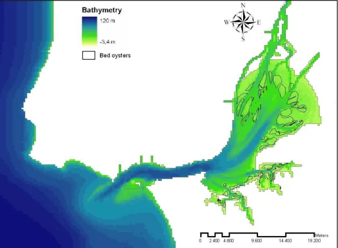
Figure 2.2 – Localization of the bed of oysters in Tagus estuary ... 16

Figure 2.3 – Relationship between tools used in this study... 17

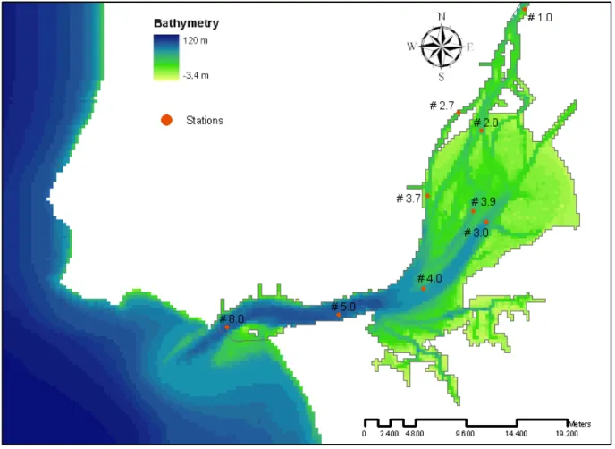
Figure 2.4 – Tagus estuary with stations... 18

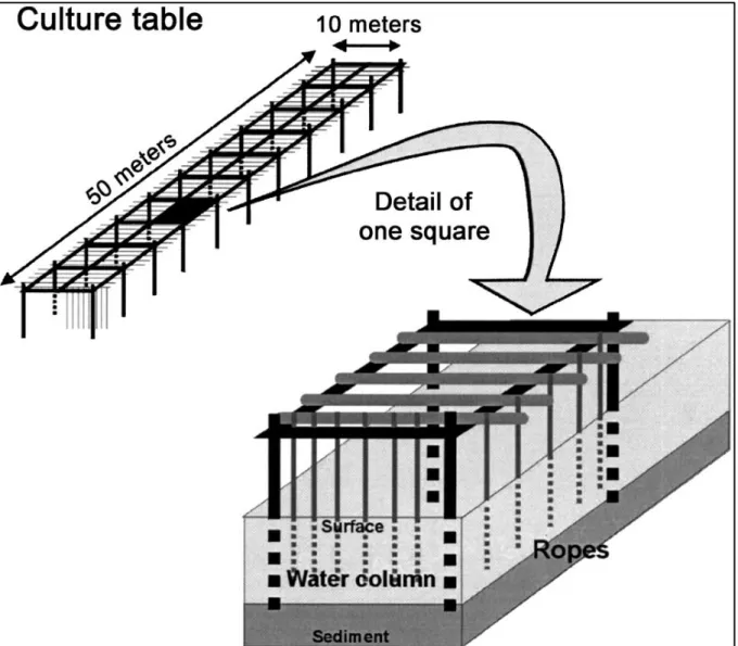
Figure 2.5 – Sketch of typical oyster table ... 19

Figure 2.6 – Tagus estuary with model box division ... 20

Figure 2.7 - Physiological components of net energy balance... 22

Figure 2.8 – Tagus estuary with model box limits and stations... 25

Figure 2.9 – Tagus estuary with the oysters’ stations... 28

Figure 3.1 – Flow: Model Calibration ... 29

Figure 3.2 – Water Temperature: Model Calibration – Box 1... 30

Figure 3.10 – Salinity: Model Calibration – Box 3 ... 35

(10)

Figure 3.16 – Salinity: Model Calibration – Box 13... 38

Figure 3.17 – SPM: Model Calibration – Box 1 ... 39

Figure 3.25 – Phytoplankton: Model Calibration – Box 1... 43

Figure 3.32 – Oyster individual weight... 47

Figure 3.33 – Oyster individual length... 47

Figure 3.34 – Oyster total harvest ... 48

Figure 3.35 – Water Temperature: Model Validation – Box 1 ... 49

Figure 3.40 – Salinity: Model Validation – Box 6... 52

(11)

Figure 3.44 – SPM: Model Validation – Box 1 ... 54

Figure 3.49 – Phytoplankton: Model Validation – Box 1... 57

Figure 3.54 – Oyster individual weight... 60

Figure 3.55 – Oyster individual length ... 60

Figure 3.56 – Oyster total harvest... 61

Figure 3.57 – Oyster individual weight: Scenario I... 61

Figure 3.58 – Oyster individual length: Scenario I... 62

Figure 3.59 – Oyster total harvest: Scenario I... 62

Figure 3.60 – Oyster individual weight: Scenario II... 63

Figure 3.61 – Oyster individual length: Scenario II... 63

(12)

(13)

(14)

(15)

Index of tables

Table 2.1 – Geographical information used in the present study... 17

Table 2.2 – Licensed area for oysters... 19

Table 2.3 – EcoWin objects implemented for Tagus estuary... 21

Table 2.4 – Values of the parameters ... 23

Table 2.5 – Performance measures for comparing model results and field data... 24

Table 3.1 – Statistics Results – Flow Calibration ... 29

Table 3.2 – Statistics Results – Water Temperature Calibration ... 30

Table 3.3 – Statistics Results – Salinity Calibration ... 34

Table 3.4 – Statistics Results – Suspended Particulate Matter Calibration ... 38

Table 3.5 – Statistics Results – Phytoplankton Calibration ... 43

Table 3.6 – Statistics Results – Water Temperature Validation... 48

Table 3.7 – Statistics Results – Salinity Validation ... 51

Table 3.8 – Statistics Results – Suspended Particulate Matter Validation... 54

(16)

(17)

(18)

(19)

1. Introduction

1.1. Problem definition

This work aims to create another alternative to fisheries economy. Over the last decades, our fish stock has been decreasing. With aquaculture, it is possible to reverse this situation.

The Tagus estuary has been chosen for this study because it provides the conditions to implement the aquaculture of bivalves, as existed for decades, until the collapse 35 years ago of the fishery of the Portuguese oysterCrassostrea angulata.

It was developed an ecological model, which integrated the physical and biogeochemical processes as well as population dynamic conditions for the oyster's growth. This model can estimate the carrying capacity of this place.

1.1.1. Aquaculture worldwide

World aquaculture has grown considerably during the last fifty years. In the 1950s the production was less than a million tonnes and in 2004 it was 59.4 million tonnes, of which 69.6% were accounted for by China, 21.9% by Asia (excluding China) and the Pacific, 3.5% by the Western Europe, 2.3% by Latin America and the Caribbean, 1.3% by North America, 0.9% by Near East and North Africa, 0.4% by Central and Eastern Europe and 0.2% by Sub-Saharan Africa. The sector has grown at an average of 8.8% per year since 1970 (FAO, 2006).

According to FAO (2001), shellfish and finfish aquaculture also has grown significantly over the last two decades. The first one, perhaps, is the most sustainable form of mariculture because it is largely extensive, requiring no artificial food input and because the animals obtain all their nutrition from phytoplankton, microphytobenthos and different types or organic detritus (Nunes, et al., 2003).

(20)

as the increase of biodeposition may contribute to significant environmental changes such as sediment anoxia (Nunes, et al., 2003).

Aquaculture is a diverse sector spanning a range of aquatic environments spread across the world, which utilizes a variety of production systems and species. It is important to recognise the problems of the impact of aquaculture such as:

 the discharge or aquaculture effluent leading to degraded water quality and organic matter

rich sediment accumulation in farming areas;

 alteration or destruction of natural habitats and the related ecological consequences of

conversion and changes in ecosystem functions;

 competition for the use of freshwater;

 introduction and transmission of aquatic animal diseases through poorly regulated

translocations; and

 effects on wildlife through methods used to control predation of cultured fish.

Over the last years, the public pressure as well as commercial pressure or common sense has led the aquaculture sector to improve management and when it is well planned and well managed it is recognized that aquaculture has positive societal benefits (FAO, 2006).

1.1.2. Aquaculture in Portugal

(21)

industry, problems such as an incomplete legislator coverage and the inability to achieve recognition as an important sector of the economy affects this activity (Bernardino, 2000).

Figure 1.1 – Shell deposits in Tagus estuary

In Portugal, aquaculture systems and operational procedures are similar to those of the Mediterranean type (Bernardino, 2000) being the production essentially exported to France.

Vilela developed the technique of culture that was used, which involves three steps: larval attachment, spat collection and growth. According to Ruano (1997), the first step is the larval attachment, which occurs on several types of collectors, including ceramic tiles covered by a cement mixture, chains of shells, and plastic tubes that are placed on the oyster beds. Subsequently, the spat collection, where workers remove the spat that are 6 -8 months old and 2 – 4 cm long from the collectors as single oysters and place them in growout areas. The last step is the growth, where the oysters remain in the farms until they attain commercial size, at least 5 cm long. In case of water quality is poor and food is sparse, it is necessary to transfer the oysters to cleaner sites with richer water to improve quality and growth (Ruano, 1997). Cleaner sites usually have less food, given food is associated with “poorer” WQ, i.e. more chl a and more detritus. The final step (afinação) is usually in less rich waters, to clean from microrganisms, improve taste, etc.

(22)

According to National Strategic Plan 2007 to 2013 is to strengthen, innovate shows the evolution of oyster producti (Direcção-Geral das Pescas e Aquicultur

Figure 1.2 – Evolution of Oyst

1.1.3. Aquaculture Legislation

There are several legal frameworks conventions as:

 Convention for the Protection

Convention);

 Convention on the Protection of the  Convention on Biological Diversit  Convention for the Protection

Convention);

Another important framework is the Comission (a), 2000) that establishes

0 200 400 600 800 1000 1999 2000 T o n n e s o f O y st e rs

Evolution of Oy

Plan for Fisheries, one of the fourth priorities to be developing innovate and diversify the aquaculture production

production in Portugal, which have increased significantly e Aquicultura, 2007).

Evolution of Oyster Production in Portugal – Font: INE/DGRA

Aquaculture Legislation

frameworks related to aquaculture. Many of them are

Protection of the Marine Environment of the North-East

Protection of the Marine Environment of the Baltic Sea Area ( ogical Diversity (CBD);

Protection of the Mediterranean Sea Against Pollution

is the European Water Framework Directive (2000/60/EC) establishes a framework for the protection of inland

2001 2002 2003 2004 2005

Years

volution of Oyster Production in

Portugal

to be developing since tion. The Figure 1.2 significantly in 2001

Font: INE/DGRA

them are international

East Atlantic (OSPAR

ea Area (HELCOM);

Pollution (Barcelona

(2000/60/EC) (European inland surface waters,

(23)

transitional, coastal and groundwater, which apart from other things, prevents further deterioration, protects, and enhances the status of aquatic ecosystem. In addition, this framework requires Member States to assess the Ecological Status of water bodies, which means achieve one determinate status through the assessment of biological, hydromorphological and physic-chemical quality elements. Some works as Borja, et al. (2007) has been developed with this framework.

The Marine Strategy establishes a framework for the development of Marine Strategies designed to achieve good environmental status in the marine environment. This shall be developed and implemented n order to:

a) Protect and preserve the marine environment, prevent its deterioration or, where practicable, restore marine ecosystems in areas where they have been adversely affected; b) Prevent and reduce inputs in the marine environment, with a view to phasing out pollution,

to ensure that there are no significant impacts on or risks to marine biodiversity, marine ecosystems, human health or legitimate uses of the sea.

Marine strategies shall apply an ecosystem-based approach to the management of human activities, ensuring that the collective pressure of such activities is kept within levels compatible with the achievement of good environmental status and that the capacity of marine ecosystems to respond to human-induced changes is not compromised, while enabling the sustainable use of marine goods and services by present and future generations (European Comission (b), 2008).

1.1.4. Carrying Capacity

Carrying capacity is a fundamental concept in shellfish culture, which corresponds to the ability of the system support shellfish production.

(24)

overall ecosystem function”. In Nunes et al. (2003) the concept of ecological carrying capacity is derived from the logistic growth curve in population ecology, defined as the maximum standing stock that can be supported by an ecosystem for a given time. This concept is not only important for species cultivation but also for other concerns such as water quality and tourism (Duarte, et al., 2003).

In this work, it is adopted the definition proposed by Inglis et al. (2000), who divided carrying capacity into four functional categories:

i. Physical Carrying Capacity – the total area of marine farms that can be accommodated in the available physical space;

ii. Production Carrying Capacity – the stocking density of bivalves at which harvests are maximized;

iii. Ecological Carrying Capacity – the stocking or farm density which causes unacceptable ecological impacts;

iv. Social Carrying Capacity – the level of farm development that causes unacceptable social impacts.

The physical carrying capacity depends on the overlap between the physical requirements of the target species and the physical properties of the area of interest, which also include some basic chemical variables like salinity and dissolved oxygen concentration. It also depends on the culture technique. Relatively to the production carrying capacity, it might be measured in terms of wet or dry weight, energy or organic carbon (McKindsey, et al., 2006).

(25)

reasons, in line with the concept of ecological aquaculture, bivalves may be successfully cultured alongside kelp, when nutrients excreted and egested may be absorbed by macroalgae and recycled into valuable biomass, according to Fang et al. (1996) (Duarte, et al., 2003).

1.1.5. Ecological models

According to Héral et al. (1986), global models allow the overall production of a system to be represented as an empirical function of the biomass (Raillard, et al., 1994). However, it is very restrictive to the carrying capacity.

Usually, spatially resolved ecological models simulate hydrodynamic transport in a very simple way, considering residual flows and tidally averaged situations (Duarte, et al., 2003). These are known as box models. Modelling has been used by different authors like Gerritsenet al. (1994), Raillard and Menesguen (1994), Ferreira et al. (1998), Bacher et al. (1998), Chapelle et al. (2000), Gangnery et al. (2001), Niquil et al. (2001) and Grillot et al. (1996), as an approach to examine environmental sustainability and to establish carrying capacity of shellfish aquaculture and is acknowledge as a powerful tool to support sustainable management (Nunes, et al., 2003).

Models are commonly used for determination of optimal carrying capacity, connecting physical processes, biogeochemistry and population dynamics offering a great potential for simulating the biomass of commercially important species under natural and cultured conditions (Franco, et al., 2006).

(26)

1.2. State of art

During the period 1962-1971, Portugal exported annually over 7500 tonnes of oysters for relaying in other countries (Ramos, 1982). All cultivation in the Tagus estuary had been carried out on the intertidal areas but sometimes was commonly to be found Crassostrea angulatain other areas like the sub-littoral zones below low tide level (Key, 1981).

Bivalve production is good in areas that have good environments with good water quality. The capacity to produce bivalves was lost completely in the Tagus estuary because of, according to Ruano (1997), the manufacturing industries, agriculture, tourist facilities, and other activities that were introduced into it.

After the 1860’s some measures were taken to improve oyster quality in the natural beds but the oyster culture only had been practiced in the middle of the 20thcentury.

The first law was passed in 1868 to regulate fishing in the natural oyster beds. It specified that:

1) Oysters could not be harvested from 1 April to 31 September, covering the spawning season;

2) the minimum size of oyster that could be harvested was 5 cm, and;

3) oysters in intertidal zones could be gathered only by hand.

Subsequently, several measures were passed covering special situations to protect human health. In 1895 the first “Regulation law for the oyster industry, oyster parks, and oyster culture” appeared. In 1923 the first “Sanitary regulation law of oyster industry” was passed. In 1953, the government built the first depuration plant for oysters in the Tagus estuary and in 1972 it was published the new “Regulation law for the oyster industry” (Ruano, 1997).

(27)

to several kilometres upstream. It can occur on substrates of sand, sandy mud, silt, and shells (Ruano, 1997).

The Oysters Mortality

Since 1973, the Portuguese oyster experienced an unexpected and extensive mortality that leads to the ending of production in the Tagus estuary and around 1974 it had occurred in France and England on such a scale that the trade was no longer economic.

According to Vilela (1975), pollution was the main reason for decline of the oyster industry, particularly in the most productive areas. One of the causes was attributed to the introduction and uses of an anti-fouling agent the tri(n-butyl)tin (TBT) by shipyards, which levels of TBT were relatively high in the open Tagus estuary and in docks (Bettencourt, et al., 1999).

Other factor that made the production of oysters declined was the occurrence of several epizootics, namely the “oyster gill disease”, which according to Comps et al. (1976) is caused by an iridovirus. This disease reduced the filtering capacity and killed some young and stressed animals. Associated to this problem was the phenomenon of abnormal shell growth. The reduction in growth of shell edges and thickening of the two surfaces of the shell with multiple layers, resulted in very heavy shell weight in relation to the overall size of the shell and of the oyster contained within it (Key, 1981).

In addition to those factors the “foot disease”; several protozoan diseases; an ineffective or absent management strategy to protect the natural beds; overharvesting and depletion of the beds by fishermen and non-existence of hatcheries; which could had provided farmers with juvenile oysters when natural spatfalls were declining, increase the mortality of the oysters (Ruano, 1997).

(28)

Estuaries

According to the definition of Pritchard (1967), an estuary is a semi-enclosed coastal body of water which has a free connection with the open sea and within which seawater is measurably diluted with fresh water derived from land drainage (Lazier, 2006). Perillo (1995) develops another further definition as, an estuary is a semi-enclosed coastal body of water that extends to the effective limit of tidal influence, within which sea water entering from one or more free connections with the open sea, or any other saline costal body water, is significantly diluted with fresh water derived from land drainage, and can sustain euryhalines biological species for either part or the whole of their life cycle (Dyer, 1997).

Estuaries are intensively used for aquaculture in many countries, and suspension-feeding bivalves are among the most cultivated organisms in these ecosystems. This is a “passive” type of culture, where the animals feed on natural suspended matter and their metabolites being dispersed by currents and waves (Duarte, et al., 2003).

Estuaries are also economically important features of the ocean because of their high biological productivity, their proximity to large cities with their wastes, and their increasing use as sites for aquaculture (Lazier, 2006).

(29)

Mesotidal estuaries, like Tagus from the turbulence of the sea,

tidal currents which ensure an intensive renewal

Estuaries can be distinguished amplitudes of different parameters substances, nutritive salts, turbidity energetic transfers. The Crassostrea their nutritional requirements well

Crassostrea angulata

In this is study it is used the Portuguese family of oysters Ostreidae. Many about their taxonomy, which

Bivalves are poecilosmotics, which than these of external seawater important to the oysters’ growth.

As well as the other suspension systems. Their biodeposits, like extremely important in regulating

Tagus estuary, are favourable areas for shellfish culture. the sea, this type of estuaries offer good trophic conditions

re an intensive renewal of food within the area (Raillard, et al.,

distinguished by the instability of environmental conditions, parameters such as tides, temperature, salinity, dissolved salts, turbidity and also by the multiplication of the various

Crassostrea are especially well adapted to those fluctuant

rements well covered in estuarine environment (Lubet, et

he Portuguese oyster, Crassostrea angulata (Figure e. Many authors as Esperança (1981/1982) and Vilela ch for this work is not given much importance.

Figure 1.3 – Image of Crassostrea angulata

motics, which means that the concentration of the body seawater (Lubet, et al.). Therefore, the environmental oysters’ growth.

suspension-feeding bivalves, oysters play an important ts, like filter suspended particles and the undigested

lating water column processes (Newell (a), 2004).

shellfish culture. For being protect trophic conditions due to strong

(Raillard, et al., 1994).

conditions, variations in great dissolved oxygen, organic various allowing important those fluctuant conditions and (Lubet, et al.).

Figure 1.3), which is from the and Vilela (1975) had written

body fluid being the same environmental conditions are very

important role in the aquatic undigested remains, could be

(30)

Crassostrea angulata is euryhalines but salinity influence respiration, nutrition, gametogenesis, growth, larvae survival and the effects are different according to the age or some environmental factors (e.g. temperature, dissolved oxygen) (Lubet, et al.). It tolerates a wide salinity range, even as low as 2-6‰ in winter and after heavy rains. It is shown that after 1-2 months of rains, a large number of oysters in the upper parts of estuaries become affected by so-called “fresh water edema” due to osmo-regulatory dysfunction. In contrast, during summer, in beds close to river mouths or inside lagoons, salinities can rise to 35-38‰ without any apparent stressing of the oyster (Ruano, 1997).

The growth of Crassostrea angulatais null under 10ºC and can survive in an aerobiosis during 10 days at 140 – 150C and more at low temperatures. Filtration stops at 80C (Lubet, et al.). The temperature range in its habitat varies from a minimum of 80-100C in northern waters during winter to 200-300C in southern lagoons during summer (Ruano, 1997).

Oysters are filter feeders, animals feeding on planktonic algae, organic particles and also bacterias, which are in good conditions for nutrition and growth in estuarine environment (Lubet, et al.).

During the rainy season, the water in large estuaries carries a large quantity of silt. It flocculates and settles on oyster beds, causing mud blisters in the shells of oysters as well as heavy mortalities of oyster spat (Ruano, 1997).

The main oyster predators are several species of crabs (especially the green crab, Carcinus maenas), gastropods, sea stars, and sea birds. Generally, oyster larvae are eaten by jellyfish (Ruano, 1997).

Although are genetic and phenotypic differences between Crassostrea angulataand Pacific oyster,

Crassostrea gigas, they are taxonomically close (Batista, et al., 2007). For this reason, we used the

(31)

1.3. Objectives

The objective of this work is to develop and implement an ecological model, which simulates the aquaculture of oysters –Crassostrea angulata– in Tagus estuary.

(32)

(33)

2. Methodology

2.1. Study area

The study was carried out in the Tagus estuary, in Portugal (Figure 2.1), one of the largest estuaries in Europe, covering an area of 320 km2. The main freshwater source to the estuary is the Tagus River, having an annual average flow of 400 m3 s-1 (Alvera-Azcárate, et al., 2003). This discharge vary significantly from winter to summer so the residence time of freshwater in estuary is highly variable, ranging from approximately 6 to 65 days (Brogueira, et al., 2006). About 112 km2are intertidal areas, which 19 km2are occupied by salt marsh vegetation and 81 km2by mudflats. The average depth is 10 m (Ferreira, et al., 2004).

The Tagus estuary is mesotidal and its circulation is mainly tidally driven, with mean tidal amplitude of 2.6 m, ranging from 4.1 m in spring tides to 1.3 m in neap tides. Tides are semi-diurnal ranging between 3.56 m at high tide and 0.87 m at low tide (Ferreira, et al., 2004).

The combined factors of low average depth, strong tidal currents and low input of river water make this a well-mixed estuary, with stratification being rare and occurring in specific situations such as neap tides or after heavy rains (Ferreira, et al., 2004).

(34)

2.2. Localization of the aquaculture areas and definition in GIS

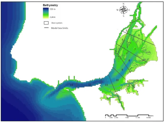
The areas where was made the study of the aquaculture viability were the oldest oysters’ bed in the Tagus estuary (Saldanha, 1980). In Figure 2.2, it is possible seen them in zones less deep.

Figure 2.2 – Localization of the bed of oysters in Tagus estuary

2.3. Loading and treatment of data

(35)

Figure

One of the tools, which have Information System (GIS). This The coordinate system used for

the Transverse Mercator Projection. The software us

Table 2.1

Layer Type

Bathymetry Sampling station data

Box definition Aquaculture areas

Coastline

Shellfish sampling stations

2.3.1. Water quality

A wide range of water quality Tagus estuary with 25 measurin various tidal situations and normally data were loaded into the relational

Station Data Aquaculture Data

ShellSIM Physiological Model

Figure 2.3 – Relationship between tools used in this study.

have already been used in aquaculture areas location This will be used again in others operations which are used for all data was UTM Zone 29N which uses the e Mercator Projection. The software used for all GIS operations was

1 – Geographical information used in the present study.

Spatial Resolution (in meters) Layer type

30 Raster (Regular grid)

- Vectorial (Points)

- Vectorial (Polygons

- Vectorial (Line)

- Vectorial (Points)

quality

quality data are available from a survey carried out during measuring stations. Typically, 30 water quality parameters and normally at three different depths (Ferreira, et al., o the relational database BarcaWin200TMand used in this work.

Relational Database

BarcaWin2000 Station location Aquacultu

Information System

Ecological Model EcoWin2000

d in this study.

location, is the Geographical which are shown in Table 2.1. the WGS-1984 Datum and operations was ESRI ArcGIS 9.2.

esent study.

Layer type Data type

Raster (Regular grid) Real Vectorial (Points) Integer Vectorial (Polygons) Integer Vectorial (Polygons) Integer Vectorial (Line) Integer Vectorial (Points) Integer

during 1980-1983 on the parameters were measured at (Ferreira, et al., 2004). The existing and used in this work.

(36)

This database, which is written in Turbo Pascal for Windows and C++, and uses the Borland Paradox Engine for all database-related functions, includes a program for file conversion between different formats, the data files and database software for analysis and exploration of the data (Ferreira, et al., 1998).

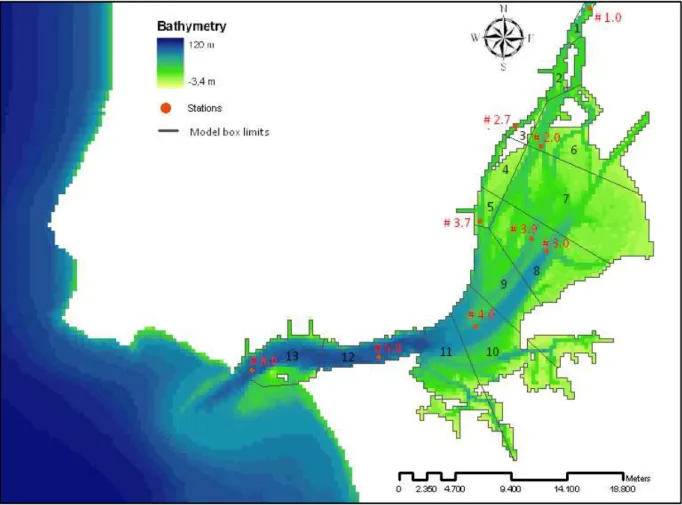
The sampling stations used in this work are shown in Figure 2.4.

Figure 2.4 – Tagus estuary with stations

2.3.2. Grow and techniques of culture

(37)

Next illustration (Figure 2.5) was extracted from Gangnery (a) et al. (2003), and it is a sketch of a typical oyster table. This type of culture consists in tables that are made of railway bars pushed in the sediment, where is supported horizontal iron bars from which the ropes are suspended in the water column. The ropes length varies depending on water deeph.

Figure 2.5 – Sketch of typical oyster table

For each box, it was calculated through GIS the licensed areas of oysters. Those are shown in Table 2.2.

Table 2.2 – Licensed area for oysters

Box 4 5 6 7 8 9 10 11

Licensed Area for

(38)

2.4. Application of ecological model

The ecosystem was assumed to be vertically homogeneous, such as Ferreira, et al. (1998), and divided into compartments. The estuary was divided into 13 ecological boxes, which could be seen in Figure 2.6, and it was used an upwind 1-D transport scheme to calculate the transport of particulate and dissolved substances between boxes.

Figure 2.6 – Tagus estuary with model box division

(39)

Table 2.3 – EcoWin objects implemented for Tagus estuary

Object type Object name Object outputs

Forcing functions

Flow Main flow

Light Total and photosynthetically active radiation (PAR) surface irradiance Air temperature Air temperature

Tide object Tidal height

Water temperature Water temperature

State variables

Hydrodynamics 1D Salinity

Nutrients Ammonia, nitrite, nitrate, phosphate silica and dissolved inorganic nitrogen (DIN) Suspended matter Suspended matter, particulate organic

matter (POM) and particulate organic carbon (POC)

Phytoplankton Phytoplankton biomass

Zoobenthos Oyster density, biomass, single individual weight and length, phytoplankton uptake and licensed area for oysters

Man Oyster total seed and harvest

For this study, the full EcoWin2000 model runs with eleven different objects, containing 23 forcing functions and 59 state variables. These simulate the relevant biogeochemistry and provide the appropriate drivers for the ShellSIM individual growth formulations (Ferreira, et al., 2008).

These drivers, known as “forcing functions”, with potential to affect physiological responses simulated by ShellSIM include food availability, food composition, seawater temperature, salinity and aerial exposure. Data required by ShellSIM to compute food availability and composition include measures of the suspended availabilities of total particulate matter (TPM; mg/l), particulate organic

matter (POM; mg/l) and Chlorophyll a (CHL; g/l) (Hawkins, 2008).

(40)

challenges by successfully simulating

across broad natural ranges of environment 2008). This software is a simple hands suspension-feeding shellfish exposed of net energy balance (Figure 2.7).

Figure 2.7 - Physiological com

The population dynamics was simulated trough simulates the transition of the shoots

density per unit area. The equation (1) expresses th

Where,

 t, time;

 s, weight class;

 n, number of shoots;

 g, scope for growth (growth rate);

 µ, mortality rate.

The parameters used are shown in table below (

simulating dynamic adjustments in feeding, metabolism environmental variability in 8 shellfish species to simple hands-on tool, calibrated to predict physiological

exposed to full natural environmental variations, based

Physiological components of net energy balance

simulated trough a class transitional model (Simas, et shoots between weight classes in order to describe plant ation (1) expresses the class transition:

owth rate);

ed are shown in table below (Table 2.4).

metabolism and/or growth s to date (Hawkins, physiological responses of based upon principles

(Simas, et al., 2007), which describe plant population

(41)

Table 2.4 – Values of the parameters

Object Parameter Value

Water Temperature Minimum temperature 9,9 ºC

Maximum temperature 24 ºC

Phase 150

Light Cloud Cover 0,5

Cloud Amplitude 0,3

Cloud Peak 350

Cloud Phase 180

Suspended Matter Turbulence 0,5 (calibrated value)

Latitude 39 ºC

Salinity 15 psu

Temperature 15 ºC

POC fraction 0,043

Phytoplankton ThresholdNH4 1µmol L

-1

kNH4 2 µmol L

-1

Pmax 0,2 h-1(calibrated value)

Ks 4 µmol L-1(calibrated value)

Iopt 450 (calibrated value)

Death loss 0,8 (calibrated value)

q10PH 0,05

RTMPH 5

Zoobenthos Number of oyster classes 10

Oyster class amplitude 10 g TFW ind. Oyster mortality 5,48 x 10-4d-1

Man Oyster first seeding day 120 d

(42)

2.4.1. Calibration

Model calibration is a critical phase in the modelling process and is done by comparing model results

with measurements and adjusting the structure and parameters of the model such that the model

results and observations match adequately (Janssen, et al., 1995). For this comparison, were used

qualitative techniques based on visual inspection of the results, as well as quantitative techniques

that express the agreement between model and data numerically. The performance measures used

in this model calibration were the Average error (AE), Relative mean bias (rB) and Correlation

Coefficient (r), which formulas are expressed below, Table 2.5:

Table 2.5 – Performance measures for comparing model results and field data.

Symbol Formulation

AE ∑

Rb

R

∑

∑ · ∑

Where,

• Pi and Oiare the model value and field data value;

• an

•

d , are their means and;

the variance of field data value.

After crossing the GIS information with the location of the stations and ecological model boxes, it

(43)

Figure 2.8 – Tagus estuary with model box limits and stations

2.4.1.1. Forcing Functions

Water Temperature

Measured water temperature from Database 1980 was used for the calibration of the water temperature. Data from stations #1.0, #2.0, #2.7, #3.7, #3.9, #4.0, #5.0 and #8.0 were selected which represent boxes 1, 3, 5, 6 , 8, 10, 12 and 13 that are illustrated in Figure 2.8

Light

(44)

River Flow

The river flow was calibrated with average month data from the Omnias Station (18E/04H) Database 1980 that represents the Box 1. This database can be accessed on National Information System Of Water Resources (SNIRH, 1995 - 2008).

2.4.1.2. State Variables

Salinity

For salinity calibration was used the Database 1980. This measured data are from stations #2.0, #2.7, #3.7, #3.9, #4.0, #5.0 and #8.0, as they are representative of the different boxes that are already referred.

Suspended Particulate Matter

The suspended particulate matter (SPM) was calibrated with the data field from the Database 1980, where stations #1.0, #2.0, #2.7, #3.7, #3.9, #4.0, #5.0 and #8.0 were selected.

Phytoplankton

Relatively to the phytoplankton biomass calibration it was used the data of chlorophyll a concentrations from Database 1980. The stations selected for that were #1.0, #2.0, #2.7, #3.7, #3.9, #4.0 and #5.0.

Zoobenthos

(45)

2.4.2. Validation

For the validation process it was used qualitative techniques and quantitative techniques, as are already mentioned above in calibration. Because it was fewer data, some stations would not be considered.

2.4.2.1. Forcing Functions

The only forcing function validated in this work was water temperature with data from Database 1982. For that, the stations selected were #1.0, #2.0, #3.9, #4.0 and #5.0, which represented boxes 1, 6, 8, 10 and 12 of the ecological model.

2.4.2.2. State Variables

Salinity

The salinity validation it was made with data from Database 1982, which stations #2.0, #3.9, #4.0 and #5.0 were used.

SPM

SPM was also validated with Database 1982. For it were used stations #1.0, #2.0, #3.9, #4.0 and #5.0.

Phytoplankton

Like SPM for phytoplankton biomass validation it was used the same stations from the Database 1982.

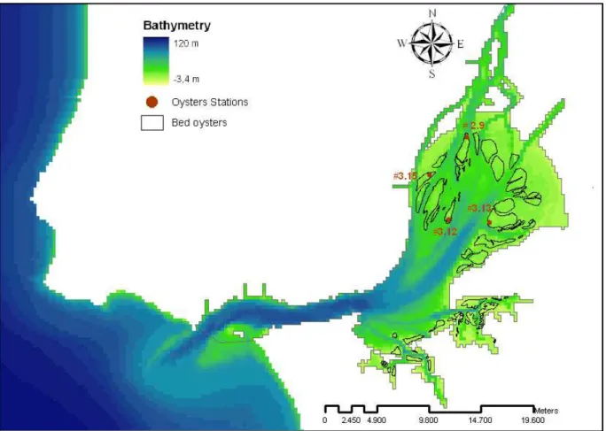
Zoobenthos

(46)

Figure 2.9 – Tagus estuary with the oysters’ stations

2.5. Scenarios

Scenario I

Global climate change is very likely to give rise to large-scale impacts on the physical and geochemical characteristics of the oceans and coast including, in addition to others, increases in sea surface temperature and sea level (European Environmental Agency, 2007). Because of that, it is chosen for Scenario I the increase of 30C on water temperature.

Scenario II

(47)

3. Results and discuss

3.1. Calibration

The calibration was made on the the results presented below were Tagus estuary.

3.1.1. Flow

Although correlation between model result error is not very high, which it is possible seen in

Table

The Figure 3.1 illustrates the expected, and in beginning considered significantly good.

100 150 200 250 300 731 781 F lo w ( m 3s -1)

iscussion

on the third year run of model, where the model was below were obtained at the end of the calibration of the

ween model results and field data do not present a good result igh, which it is possible seen in Table 3.1.

Table 3.1 – Statistics Results – Flow Calibration

Box 1

Relative Bias -0,1

Average Error (%) 36%

Correlation -0,15

the evolution of model along the year. In spring, beginning of autumn start to increase again. Therefore, cantly good.

Figure 3.1 – Flow: Model Calibration

781 831 881 931 981 1031

Time (Julian Day)

Flow

Measured Model Results

model was already stabled and of the 13 box model of the

ta do not present a good result, the average

spring, the flow decreases as Therefore, the model result is

(48)

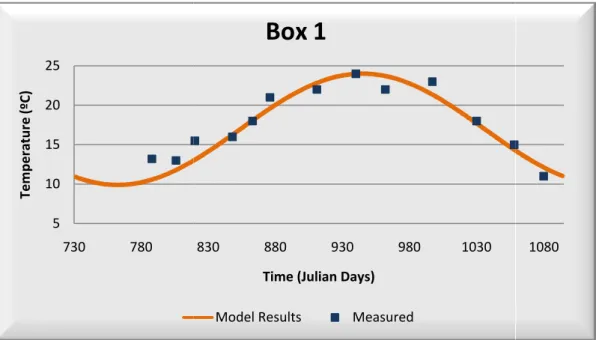
3.1.2. Water Temperature

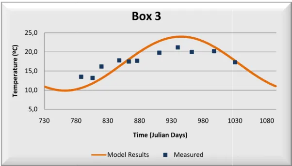
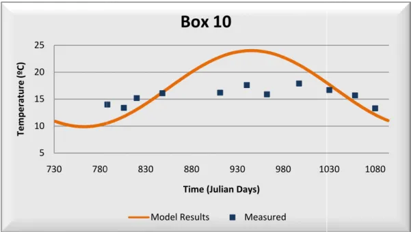
After calibration, water temperature field data as it can be seen in Table correlation coefficient higher than 0,90

the model represents very well water temperatur

Table 3.2 – Statistics Results

Box 1 Box 3

Relative Bias 0,5

-Average Error (%) 7% 12%

Correlation 0,96 0,96

The model results and measured data are pres 3.5, Figure 3.6, Figure 3.7, Figure 3.8

Figure 3.2 – Water Temp

5 10 15 20 25 730 780 T e m p e ra tu re ( ºC )

Water Temperature

temperature presents a very good correlation between model Table 3.2. The majority of the boxes used in this calibration than 0,90 as also a minor average error and relative bias,

water temperature.

Statistics Results – Water Temperature Calibration

Box 3 Box 5 Box 6 Box 8 Box 10 Box 12 Box 13

-0,4 -1,6 -0,3 -1,1 -1,4 -2,3 -2,7

12% 18% 12% 13% 20% 21% 27%

0,96 0,91 0,90 0,92 0,81 0,79 0,16

data are presented below in Figure 3.2, Figure 3.3, 8 and Figure 3.9.

Water Temperature: Model Calibration – Box 1

830 880 930 980 1030

Time (Julian Days)

Box 1

Model Results Measured

between model results and this calibration have a relative bias, which means

Box 13 Global

2,7 -1,1

27% 15%

0,16 0,77

, Figure 3.4, Figure

(49)

Figure Figure 5,0 10,0 15,0 20,0 25,0 730 780 T e m p e ra tu re ( ºC ) 5 10 15 20 25 730 780 T e m p e ra tu re ( ºC )

Figure 3.3 – Water Temperature: Model Calibration – Box 3

Figure 3.4 – Water Temperature: Model Calibration – Box 5

780 830 880 930 980 1030

Box 3

780 830 880 930 980 1030

Box 5

Box 3

Box 5

1030 1080

(50)

5 10 15 20 25

730 780

T

e

m

p

e

ra

tu

re

(

ºC

)

5 10 15 20 25

730 780

T

e

m

p

e

ra

tu

re

(

ºC

)

830 880 930 980 1030

Box 6

830 880 930 980 1030

Box 8

1080

(51)

Figure 3 Figure 3 5 10 15 20 25 730 780 T e m p e ra tu re ( ºC ) 5 10 15 20 25 730 780 T e m p e ra tu re ( ºC )

3.7 – Water Temperature: Model Calibration – Box 10

3.8 – Water Temperature: Model Calibration – Box 12

780 830 880 930 980 1030

Box 10

780 830 880 930 980 1030

Box 12

Box 10

Box 12

1030 1080

(52)

3.1.3. Salinity

Salinity is run in the model by variation salinity and the opposite happens in very good, as it is shown in Table r=0,75. Besides the bad individual

lower values, which at the end represent measured data.

Table 3.3

Box 3 Box 5

Relative

Bias 1,9 -2,1

Average

Error (%) 41% 13%

5 10 15 20 25 730 780 T e m p e ra tu re ( ºC )

variation of the river flow, which means low flow in happens in winter. Despite the individual box correlation

Table 3.3, the global variation presents a good one

individual correlation coefficient, the average error and relative end represent the satisfying relation between the

3 – Statistics Results – Salinity Calibration

Box 6 Box 8 Box 10 Box 12 Box 13

1,8 -2,3 -0,7 -0,6 1,1

37% 11% 10% 7% 4%

0,21 0,21 0,10 0,47 0,36

830 880 930 980 1030

Box 13

flow in summer, higher correlation coefficient isn’t correlation, with and relative bias have the model and the

Box 13 Global

1,1 -0,1

4% 18%

0,36 0,75

(53)

The figures below, Figure 3.10 Figure 3.16, show the model respectively. Figure Figure 0 5 10 15 20 25 30 35 730 780 S a li n it y ( p su ) 20 22 24 26 28 30 32 34 36 730 780 S a li n it y ( p su )

10, Figure 3.11, Figure 3.12, Figure 3.13, Figure model results and the measured data for boxes 3, 5,

Figure 3.10 – Salinity: Model Calibration – Box 3

780 830 880 930 980 1030

Box 3

780 830 880 930 980 1030

Box 5

Figure 3.14, Figure 3.15 and boxes 3, 5, 6, 8, 10, 12 and 13

1030 1080

(54)

Figure 3

4 9 14 19 24 29

730 780

S

a

li

n

it

y

(

p

su

)

20 25 30 35

730 780

S

a

li

n

it

y

(

p

su

)

3.12 – Salinity: Model Calibration – Box 6

3.13 – Salinity: Model Calibration – Box 8

830 880 930 980 1030

Box 6

830 880 930 980 1030

Box 8

1080

(55)

Figure Figure 25 27 29 31 33 35 37 730 780 S a li n it y ( p su ) 25 27 29 31 33 35 37 730 780 S a li n it y ( p su )

780 830 880 930 980 1030

Box 10

780 830 880 930 980 1030

Box 12

1030 1080

(56)

Figure 3.

3.1.4. Suspended Particulate

The results of SPM calibration do not This fact might result of variation from Figure 3.18, Figure 3.19, Figure 3.20

Although the results presented in Table Table 3.4 – Statistics Results

Box 1 Box 3

Relative Bias 17,4 24,1

Average Error (%) 58% 55%

30 32 34 36 38 40 730 780 S a li n it y ( p su )

.16 – Salinity: Model Calibration – Box 13

articulate Matter (SPM)

SPM calibration do not present a good correlation between model and m variation from measured data along the year, like is shown

20, Figure 3.21, Figure 3.22, Figure 3.23 and Figure

Table 3.4, the model are considered as satisfying at the year scal Statistics Results – Suspended Particulate Matter Calibration

24,1 19,5 0,4 23,3 12,2 5,2 5,4

55% 37% 33% 40% 42% 51% 35%

0,61 -0,55 0,68 -0,67 -0,17 -0,05 -0,54

830 880 930 980 1030

Box 13

on between model and measured data. wn in Figure 3.17, Figure 3.24.

g at the year scale. Calibration

Box 13 Global

5,4 13,5

35% 44%

0,54 0,46

(57)

5 25 45 65 85 105

730 780

S

P

M

5 25 45 65 85 105 125

730 780

S

P

M

Figure 3.17 – SPM: Model Calibration – Box 1

780 830 880 930 980 1030

Box 1

780 830 880 930 980 1030

Box 3

1030 1080

(58)

Figure

5 25 45 65 85

730 780

S

P

M

5 25 45 65 85 105

730 780

S

P

M

830 880 930 980 1030

Box 5

830 880 930 980 1030

Box 6

1080

(59)

10 20 30 40 50 60 70 80 90

730 780

S

P

M

10 20 30 40 50 60 70

730 780

S

P

M

780 830 880 930 980 1030

Box 8

780 830 880 930 980 1030

Box 10

1030 1080

(60)

Figure

5 15 25 35 45 55

730 780

S

P

M

5 15 25 35 45 55

730 780

S

P

M

830 880 930 980 1030

Box 12

830 880 930 980 1030

Box 13

1080

(61)

3.1.5. Phytoplankton

The correlation between model presented in Table 3.5, are considerab

Table

Box 1

Relative Bias 11,5

Average

Error (%) 56%

Correlation 0,55

The variation of phytoplankton 3.28, Figure 3.29, Figure 3.30 illustrating the bloom.

Figure 0 10 20 30 40 50 60 70 730 780 P h y to p la n k to n b io m a ss (µ g c h l a l -1)

Phytoplankton

model results and measured data, even though the , are considerably good.

Table 3.5 – Statistics Results – Phytoplankton Calibration

Box 3 Box 5 Box 6 Box 8 Box 10

-1,2 3,1 -0,6 1,6 6,4

59% 62% 102% 64% 53%

0,63 0,34 0,63 0,45 0,61

kton biomass is presented in Figure 3.25, Figure 3

and Figure 3.31, where it is possible seen the increase of

Figure 3.25 – Phytoplankton: Model Calibration – Box 1

780 830 880 930 980 1030

Box 1

though the huge errors values

Box 10 Box 12 Global

5,7 3,8

77% 68%

0,52 0,52

3.26, Figure 3.27, Figure he increase of chl a in springs

(62)

Figure 3.26 Figure 3.27 0 5 10 15 20 25 730 780 P h y to p la n k to n b io m a ss (µ g c h l a l -1) 0 5 10 15 20 730 780 P h y to p la n k to n b io m a ss (µ g c h l a l -1)

– Phytoplankton: Model Calibration – Box 3

830 880 930 980 1030

Box 3

830 880 930 980 1030

Box 5

1080

(63)

Figure Figure 0 5 10 15 20 25 30 730 780 P h y to p la n k to n b io m a ss (µ g c h l a l -1) 0 5 10 15 20 730 780 P h y to p la n k to n b io m a ss (µ g c h l a l -1)

780 830 880 930 980 1030

Box 6

780 830 880 930 980 1030

Box 8

1030 1080

(64)

Figure 3.30 –

Figure 3.31 –

0 10 20 30 40 730 780 P h y to p la n k to n b io m a ss (µ g c h l a l -1) 0 10 20 30 40 730 780 P h y to p la n k to n b io m a ss (µ g c h l a l -1)

830 880 930 980 1030

Box 10

830 880 930 980 1030

Box 12

1080

(65)

3.1.6. Zoobenthos

After calibration it can be seen overestimate oyster growth in oyster growth in all boxes, any oyster growth in the others.

0 50 100 150 200 250 300

Box 4 Box 5

W e ig h t (g ) 0 2 4 6 8 10 12 14

Box 4 Box 5

Le n g th ( cm )

Zoobenthos

be seen in Figure 3.32 and Figure 3.33 that the model growth in box 4 and 6. Because the same parameters are all boxes, any change to get better box 4 and 6 results would t

Figure 3.32 – Oyster individual weight

Figure 3.33 – Oyster individual length

Nº of the Box

Oyster Individual Weight

Nº of the Box

Oyster Individual Length

the model results tend to parameters are used to simulate the 6 results would tend to underestimate

Box 11

Weight

Box 11

(66)

At the end of third year of calibration,

Figure 3.34. It is shown that in boxes 6, 7 and 8 the

Figure

3.2. Validation

3.2.1. Water Temperature

The model results for water temperature we Database 1982 - Figure 3.35, Figure

model results still presents a good correlation with recalibrated for the validation of the model.

Relative Bias

Average Error (%)

Correlation 0 1000 2000 3000 4000 5000 6000 7000

Box 4 Box 5 Box 6

H a rv e st ( to n T F W )

Oys

calibration, the total oysters harvested for each box are shown that in boxes 6, 7 and 8 the production is higher than in the others.

Figure 3.34 – Oyster total harvest

Water Temperature

temperature were compared to the measured water temperature of Figure 3.36, Figure 3.37, Figure 3.38 and Figure 3.39

ood correlation with field data (Table 3.6) this forcing function was validation of the model.

Statistics Results – Water Temperature Validation

Box 1 Box 6 Box 8 Box 10 Box 12 Global

2,0 0,5 0,2 -0,8 -1,3 0,3

ror (%) 12% 15% 10% 13% 17% 13%

0,94 0,68 0,95 0,96 0,91 0,80

Box 6 Box 7 Box 8 Box 9 Box 10 Box 11

Nº of the Box

Oyster Total Harvest

Total Harvest

box are illustrated in the others.

temperature of the 39. Because of the this forcing function was not

Global

(67)

Figure Figure 5 10 15 20 25 1460 1510 T e m p e ra tu re ( ºC ) 5,0 10,0 15,0 20,0 25,0 1460 1510 T e m p e ra tu re ( ºC )

Figure 3.35 – Water Temperature: Model Validation – Box 1

Figure 3.36 – Water Temperature: Model Validation – Box 6

1510 1560 1610 1660 1710 1760

Box 1

1510 1560 1610 1660 1710 1760

Box 6

Box 1

Box 6

1760 1810

(68)

5 10 15 20 25

1460 1510 1560

T

e

m

p

e

ra

tu

re

(

ºC

)

5 10 15 20 25

1460 1510 1560

T

e

m

p

e

ra

tu

re

(

ºC

)

Water Temperature: Model Validation – Box 8

Water Temperature: Model Validation – Box 10

1560 1610 1660 1710 1760

Box 8

1560 1610 1660 1710 1760

Box 10

1810

(69)

Figure 3

3.2.2. Salinity

Like it was happened in salinity percentage of errors is not relevant validation model.

Table

Relative Bias

Average Er

Correlation

In Figure 3.40, Figure 3.41, Figure data for salinity validation.

5 10 15 20 25 1460 1510 T e m p e ra tu re ( ºC )

3.39 – Water Temperature: Model Validation – Box 12

in salinity calibration, in validation, the global correlation not relevant (Table 3.7), so that this state variable is not

Table 3.7 – Statistics Results – Salinity Validation

Box 6 Box 8 Box 10 Box 12 Global

Relative Bias 3,6 -1,4 -3,5 -2,6 -0,8

erage Error (%) 25% 8% 18% 14% 17%

Correlation 0,18 0,55 0,22 -0,47 0,70

Figure 3.42 and Figure 3.43 are shown the model

1510 1560 1610 1660 1710 1760

Box 12

Box 12

global correlation is good and is not recalibrated for the

Global

0,8

17%

0,70

model results and measured

(70)

Figure 3

10 15 20 25 30

1460 1510 1560

S

a

li

n

it

y

(

p

su

)

25 27 29 31 33 35

1460 1510 1560

S

a

li

n

it

y

(

p

su

)

3.40 – Salinity: Model Validation – Box 6

3.41 – Salinity: Model Validation – Box 8

1560 1610 1660 1710 1760

TítTime (Julian Days)ulo

Box 6

1560 1610 1660 1710 1760

Box 8

1810

(71)

Figure

20 25 30 35

1460 1510

S

a

li

n

it

y

(

p

su

)

20 25 30 35

1460 1510

S

a

li

n

it

y

(

p

su

)

Figure 3.42 – Salinity: Model Validation – Box 10

Figure 3.43 – Salinity: Model Validation – Box 12

1510 1560 1610 1660 1710 1760

Box 10

1510 1560 1610 1660 1710 1760

Box 12

1760 1810

(72)

3.2.3. Suspended Particulate Matter

For this state variable, the conclusion satisfactory results at the year scale. below (Table 3.8).

Relative Bias

Average Error (%)

Correlation

The model results and measured data 3.45, Figure 3.46, Figure 3.47 and Figure

Figure

0 20 40 60 80

1460 1510 1560

S

P

M

Suspended Particulate Matter

conclusion is the same that it was in calibration, the year scale. The outcomes for the quantitative validation are

Statistics Results – Suspended Particulate Matter Validation

Box 1 Box 6 Box 8 Box 10 Box 12 Global

18,1 8,9 13,7 7,1 1,0 10,1

ror (%) 39% 33% 51% 35% 24% 36%

-0,42 -0,07 -0,55 0,01 0,09 0,45

measured data are illustrated for respectively boxes in Figure Figure 3.48.

Figure 3.44 – SPM: Model Validation – Box 1

1560 1610 1660 1710 1760

Box 1

the model presents validation are shown in table

Validation

Global

Figure 3.44, Figure