UNIVERSIDADE DA BEIRA INTERIOR
Ciências Sociais e Humanas
ECONOMIC GROWTH, INFLATION AND STOCK
MARKET DEVELOPMENT: A PANEL VAR APPROACH
João Vasco Oliveira Mota
Dissertação para obtenção do Grau de Mestre em
Economia
(2º ciclo de estudos)
Orientador: Prof. Doutor José Alberto Serra Ferreira Rodrigues Fuinhas
iii
Acknowledgements
In first place I want to thank to Professor José Alberto Serra Ferreira Rodrigues Fuinhas for accepted the invitation to be my supervisor and for all the work, advises and knowledge that he has transmitted to me.
I want to express my gratitude to my family for all the support and for the opportunity to became a master in economics.
Also want to thank to all my friends that have been at my side in this long journey, without their support It would not be possible to accomplish this goal.
Finally, I want to thank all the people who I have met during this journey, and that in one way or another helped me.
v
Resumo
A relação dinâmica entre crescimento económico, inflação e desenvolvimento de mercado de capitais foi examinada para 31 países de todo o Mundo, para o período de 2000 a 2014, utilizando dados anuais. De forma a conseguir medir o desenvolvimento de mercado de capitais foi criada uma variável composta através da Análise de Componentes Principais. Para avaliar a interdependência entre as variáveis e as causalidades de Granger, foi aplicado um modelo de painel vetor autorregressivo. Este estudo distingue-se dos existentes ao utilizar uma metodologia que permite testar as hipóteses em ambas as direções nas causalidades de Granger, o que na literatura existente é escasso. Os resultados demostram a presença de causalidade bidirecional do desenvolvimento de mercado de capitais para crescimento económico; do crescimento económico para a inflação e a presença de causalidade unidirecional do desenvolvimento de mercado de capitais para a inflação. As funções de impulso resposta e a decomposição da variância mostram que a maioria dos choques exerce o seu efeito nos primeiros dois anos. Este estudo conclui que o desenvolvimento de mercado de capitais estimula o crescimento.
Palavras-chave
Crescimento económico; Painel VAR; PCA; Desenvolvimento de mercados de capitais; Inflação.
vi
Resumo Alargado
O nexus entre crescimento económico, inflação e desenvolvimento de mercados de capitais tem sido objeto de estudo nas últimas décadas. Estes estudos têm como objetivo avaliar o papel que o desenvolvimento do mercado de capitas e a inflação têm no crescimento económico. Os resultados destes estudos são heterogéneos devido a diferentes metodologias aplicadas, dados, variáveis e horizonte temporal.
Na literatura estão presentes três hipóteses: hipótese neutra quando não existe causalidade entre variáveis; hipótese supply-leading ou demand-following quando existe uma causalidade unidirecional entre variáveis; hipótese feedback quando existe uma causalidade bidirecional entre variáveis.
Nesta dissertação analisa-se a relação dinâmica entre crescimento económico, inflação e desenvolvimento do mercado de capitais em 31 países entre 2000 e 2014. Este estudo diferencia-se dos demais já realizados devido a aplicar um painel vetor autorregressivo que trata todas as variáveis como endógenas e permite observar heterogeneidade individualmente.
Para medir o crescimento económico foi utilizado a variável produto interno bruto per capita a preços de 2005. A variável inflação é reportada ao final do período usando o índice de preços no consumidor. Para medir o desenvolvimento de mercado de capitais foram utilizadas duas variáveis: rácio de capitalização de mercado (capitalização de mercado dividido pelo produto interno bruto, com valores nominais) e Turnover ratio (valor das ações das empresas cotadas em bolsa a dividir pelo produto interno bruto, valores nominais) criando-se uma variável composta que incorpora a informação importante de cada uma das variáveis usadas, transformando-a numa só varável através da análise de componentes principais. Todas as variáveis encontram-se na forma de logaritmos naturais.
Foram realizados testes de cross-section e posteriormente testes de 2ª geração de raízes unitária devido a presença de cross-section dependece. Testamos o modelo através do teste de Hausman para saber se é um modelo de efeitos fixos ou aleatórios. Aplicou-se um painel vetor autorregressivo, seguidamente testou-se a causalidade entre variáveis através do teste de Granger. Apresentamos as funções de resposta-impulso, permitem observar os efeitos de um choque de uma variável endógena sobre as restantes variáveis, e a decomposição da variância do erro de previsão, demonstra o comportamento de cada uma das variáveis na explicação da variância das restantes variáveis do modelo após um choque.
vii
Os resultados obtidos neste estudo corroboram a hipótese feedback, entre crescimento económico e inflação, e entre crescimento económico e desenvolvimento do mercado de capitais. Existe ainda a presença de uma causalidade unidirecional entre desenvolvimento de mercado de capitais e inflação, hipótese supply-leading.ix
Abstract
The dynamic relationship between economic growth, inflation and stock market development was examined for 31 countries from the entire world, for the period from 2000 to 2014, by using annual data. In order to better measure the stock market development a composite variable was created through the principal component analysis. To assess the interdependence among the variables, and Granger causalities, a panel vector auto-regressive model, was estimated. This research differs from the others by using a methodology that allows testing the hypotheses in both directions in Granger casualties, which is scarce in literature. The study finds bi-directional causality running from stock markets development to economic growth, from stock markets development to inflation and a unidirectional causality from economic growth to inflation. The impulse response functions and the forecast-error variance decomposition show that most of the shocks exert their effect during the first two years. The research supports that the development of stock markets stimulates economic growth.
Keywords
xi
Index
1. Introduction ... 1
2. Literature Review ... 2
3. Data and Methodology ... 3
3.1. Data ... 3
3.2. Methodology ... 5
3.3. Preliminary tests ... 5
4. Empirical Results ... 8
5. Conclusion ... 12
References ... 13
xiii
Figures list
xv
Tables list
Table 1. Variables description and summary statistics Table 2. Factortest LMCAP LTUR
Table 3. VIF test and Average correlation coefficients & Pesaran CD test Table 4. Panel Unit Root test (CIPS)
Table 5. Hausman Test
Table 6. Lag order selection on estimation Table 7. VAR model Results
Table 8. Panel VAR-Granger causality Wald test Table 9. Forecast-error variance decomposition Table 10. Eigenvalue stability condition
xvii
Acronyms list
GDP Gross Domestic Product PVAR Panel vector Autoregressive PCA Principal Component Analysis CIPS Cross-sectionally augmented IPS GMM Generalized method of moments SDM Stock market development
INF Inflation
TUR Turnover ratio
MCAP Market capitalization of listed domestic companies VIF Variance inflation factor
1
1. Introduction
Since the beginning of the existence of stock markets had an important role in the economy. When stock markets started did not traded real stocks but promissory notes and bonds. With the increase of the demand was necessary to organize a marketplace where people could make their trades people used to go to a coffee shops where the debt issues and shares sales were fixed in the coffees doors or mailed as a newsletter. From there to the creation of an official stock market exchange was just a question of time due the necessity of regulation and the increase of the volume of trade stocks. Due the importance that a stock market has in the economy of a country researchers have turn their attention to study how a stock market influence economic growth. In the last decades, the relationship between economic growth, inflation and Stock market development has been object of many studies. The results of this studies are heterogeneous, hence that every study uses different methodology, data and time span. In this study the variables used were Real Gross Domestic (as a proxy of economic growth), Inflation and to measure stock market development was used a composite variable created from market capitalization of listed domestic and turnover ratio. This kind of issues usually was studied by using two variables with time series, in this study a Panel Vector Autoregressive approach was used which allows to use all the variables at the same time. Using a panel constituted by 31 countries worldwide with a time span from 2000 to 2014. The empirical research of casual relationship between economic growth, inflation and stock market development showed significance causality between these variables. Thought the analysis of Impulse-Response functions and variance decomposition revealed the impact that each variable has in the others.
The rest of this paper is organized as follow: Section 2 presents a literature review and the main contributes. Section 3 describes data, methodology and preliminary tests. Discussion is presented in Section 4 and Section 5 concludes.
2
2. Literature Review
This paper follows the literature existence by studding the presence of causality between economic growth, inflation and stock market development. There is in literature different conclusions about the direction of the causality between these variables what can be justified due to different methodology, data and time period applied in each study. There are three hypotheses in literature: the neutral hypothesis meaning there is no causality between variables, the supply-leading or demand-following hypothesis when is a unidirectional causality among two variables, and the feedback hypothesis when there is a bidirectional causality between variables. Is expected that stock market development have a positive impact on economic growth (e.g. Capasso, 2008; Levine and Zervos, 1998).
A review of literature shows that the supply-leading hypothesis, unidirectional causality from stock market development and economic growth, is supported by Enisan and Olufisayo (2009), Kolapo et al. (2012), Pradhan et al. (2013).The demand-following hypothesis, unidirectional causality from economic growth to stock market development is founded in Kar et al. (2011), Panopoulou (2009), Liang and Teng (2006). Supporting the feedback hypothesis, bidirectional causality among stock market development and economic growth, there is the studies of Cheng (2012), Hou and Cheng (2010), and Zhu et al. (2004). Supporting the neutral hypothesis is the study of Lu and So (2001).
In the relationship between Inflation and stock market development the supply-leading hypothesis, unidirectional causality from inflation to stock market development, is supported by Dritsaki and Bargiota (2005). The demanding-following hypothesis, unidirectional causality from stock market development to inflation, is supported by Liu and Sinclair (2008), Shahbaz et al. (2008), and Zhao (1999). The feedback hypothesis, bidirectional causality among stock market development and inflation, is supported by Cakan (2013), and Pradhan (2011). Supporting the neutral hypothesis, Lu and So (2001), there is no casual links between inflation and stock market development.
Supporting the supply-leading hypothesis, inflation causes economic growth, is Pradhan et al. (2013). Demanding-following hypothesis, unidirectional causality from economic growth to inflation (Kim et al., 2016). The Feedback hypothesis is supported by Nguyen and Wang (2010), and Kar et al. (2011). The neutral hypothesis, no casual links between variables, is supported by Billmeier and Massa (2009).
3
3. Data and Methodology
This section is divided in three subsections. In the first one the variables and data used are described. The second subsection contains the method used. The third subsection show the preliminary tests.
3.1. Data
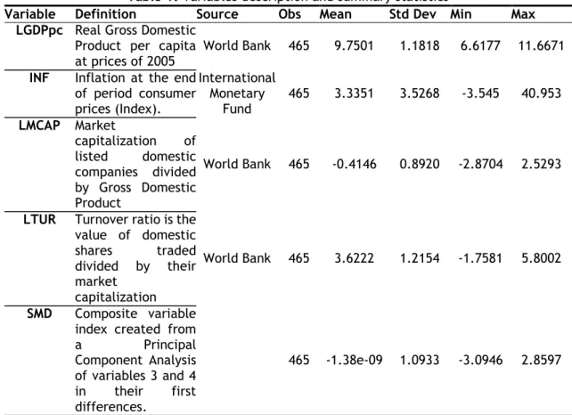
Annual data from 2000 to 2014 was applied to a panel of 31 countries: Argentina, Austria, Australia, Belgium, Canada, Chile, France, Germany, China (Hong Kong SAR), Indonesia, Ireland, Israel, Japan, Korea Republic, Luxemburg, Malaysia, Mexico, the Netherlands, Norway, Peru, Philippines, Poland, Portugal, Singapore, Slovenia, South Africa, Spain, Sri Lanka, Switzerland, Thailand and the United States. The variables Real Gross Domestic Product per capita, Inflation, Market Capitalization and Turnover Ratio. The criteria used to select the time horizon and the countries was the data available. The Table 1 show name, definition, source raw data and the summary statistics of the variables.
Table 1: Variables description and summary statistics
Variable Definition Source Obs Mean Std Dev Min Max
LGDPpc Real Gross Domestic Product per capita at prices of 2005
World Bank 465 9.7501 1.1818 6.6177 11.6671 INF Inflation at the end
of period consumer prices (Index). International Monetary Fund 465 3.3351 3.5268 -3.545 40.953 LMCAP Market capitalization of listed domestic companies divided by Gross Domestic Product World Bank 465 -0.4146 0.8920 -2.8704 2.5293
LTUR Turnover ratio is the value of domestic shares traded divided by their market capitalization World Bank 465 3.6222 1.2154 -1.7581 5.8002 SMD Composite variable index created from a Principal Component Analysis of variables 3 and 4 in their first differences. 465 -1.38e-09 1.0933 -3.0946 2.8597
Notes: The prefixes L and D denote natural logarithms and the first differences, respectively; all the monetary values are in US Dollars.
4
To measure economic growth was used Real Gross Domestic Product per capita at prices of 2005 in natural logarithms, the data was obtained from the World Bank (Code: NY.GDP.PCAP. KD). Inflation data was obtained from International Monetary Fund and is reported to the end of the period consumer prices (Index).To measure Stock Market Development was used the variables Market Capitalization of listed domestic companies and Turnover Ratio of domestic shares both obtained from the World Bank (Code: CM.MKT.LCAP.CD and CM.MKT.TRNR respectively), in order to use only one variable and due to both variables have much in common was created a composite variable, SMD, using Principal Component Analysis (PCA). The use of PCA allow removing the essential information that each variable gives and turn it into a single variable that incorporate information from both variables. To test the robustness of the composite variable was performed the test of Kaiser-Meyer-Olkin measure of sampling adequacy (Kaiser 1970), and Bartlett's test for sphericity (Bartlett 1950) using the Stata command factortest (see Table 2).
Table 2: Factortest LMCAP LTUR
Determinant of the correlation matrix 0.962 Bartlett test of sphericity
Chi-square 18.003
Degrees of freedom 1
p-value 0.0000
Kaiser-Meyer-Olkin measure of sampling adequacy 0.5
The determinant of the correlation matrix is less than one when all correlations are different than zero, if all correlations are equal to zero then the value of the determinant of the correlation matrix is one, in this case the value of the determinant of the correlation matrix is 0.962 meaning that all the measures are correlated.
The Bartlett test of sphericity has as null hypothesis that the variances are equal, in this case the null hypothesis was not rejected.
Kaiser-Meyer-Olkin measure of sampling adequacy is an index, between zero and one, of the magnitudes of the variance among the variables that might be common variance. If the value is below 0.5 is considerable unacceptable and PCA should not be made. In this case the value of Kaiser-Meyer-Olkin measure of sampling adequacy is 0.5, is considerable miserable, but is possible to use PCA.
5
3.2. Methodology
To analyse the relation between all the variables was applied a panel-data vector autoregressive (PVAR) model developed by Love and Zicchino (2006). In this model, all the variables are treated as endogenous and unobserved individual heterogeneity was allowed (Grossmann et al., 2014). All variables are stationary in their first differences (see table 4). The first-order PVAR model equation is showed in eq.1:
t t c it it
z
d
z
0
1 1
f
i
,
(1)where is the vector for the tree variables used in our study: DLGDPpc, DINF and DSMD denotes the vector of constants; denotes the matrix polynomial; denotes the fixed effects (was performed the Hausman test to confirm); denotes time effects and denotes the random errors term. Due the fact that the model use fixed effect that, cause correlation between the fixed effects and the regressors, that result of the lags of the depended variables, was applied the technique known as the “Helmert procedure” (Arellano and Bover, 1995). Only was removed the forward mean-differencing, i.e. the mean of all the future observations available for each country-year (Love and Zicchino, 2006). Using Generalized method of moments (GMM), with the lags of the regressors as instruments, the system was estimated. Granger causality test was performed to analyse the casual relationship between the variables, the variance decomposition shows the percent of the variation in one variable that is explained by the shock to another variable that accumulate over time. The variance decomposition was performed by 10 periods. Impulse-response functions describes the reaction of one variable to the innovation in another variable in the system (e.g. Papadamou et al., 2015). The impulse-response function was compute by follow Choleski procedure. Standard errors of impulse-response and the confidence-intervals were estimate by Monte Carlo simulations (the procedure was repeat 1000 times to compute the 5th and the 95th percentiles of the impulse responses).
3.3. Preliminary tests
This section shows the preliminary tests on data to check the proprieties of the variables. To teste the multicollinearity was performed the Variance Inflation Factor test (VIF) and to test for Cross-section was performed the Pesaran CD test (Pesaran, 2004). The results of both tests can be seen in Table 3.
6
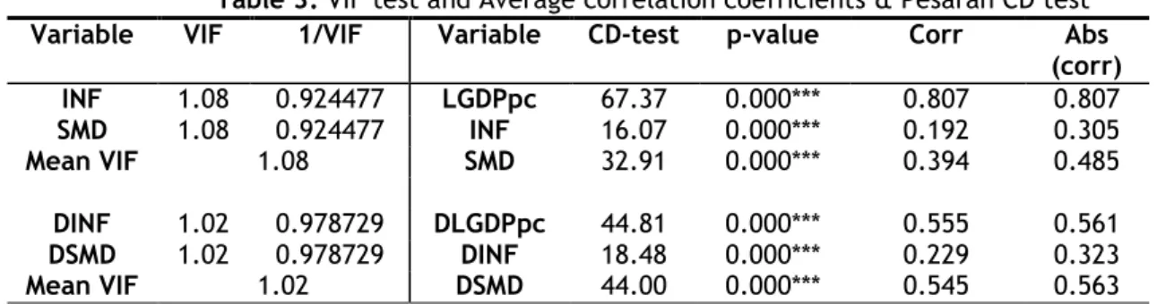
Table 3: VIF test and Average correlation coefficients & Pesaran CD testVariable VIF 1/VIF Variable CD-test p-value Corr Abs
(corr) INF 1.08 0.924477 LGDPpc 67.37 0.000*** 0.807 0.807 SMD 1.08 0.924477 INF 16.07 0.000*** 0.192 0.305 Mean VIF 1.08 SMD 32.91 0.000*** 0.394 0.485 DINF 1.02 0.978729 DLGDPpc 44.81 0.000*** 0.555 0.561 DSMD 1.02 0.978729 DINF 18.48 0.000*** 0.229 0.323 Mean VIF 1.02 DSMD 44.00 0.000*** 0.545 0.563
Notes: *** denotes statistical significance level of 1%; The Stata command xtcd was used.
At level the value of the mean of VIF was 1.08 and at the first differences was of 1.02. In both cases the value of VIF is lower than 10, meaning that multicollinearity between variables is not a concern. The null hypothesis of the CD Pesaran test is cross-section independence CD ~ N(0,1), in this case, there is cross-section dependence in levels and at the first differences. Due to the fact that there is cross-section dependence only was executed the 2nd generation of unit root test, cross-sectionally augmented IPS (CIPS) test (Pesaran 2007). The results can be seen in Table 4.
Table 4: Panel Unit Root test (CIPS)
Specification without trend Specification with trend
Variable Zt-bar p-value Zt-bar p-value
LGDPpc 0.647 0.741 0.095 0.538 INF -5.018 0.000*** -3.140 0.001*** SMD -1.219 0.111 -2.385 0.09 DLGDPpc -4.727 0.000*** -1.878 0.000*** DINF -12.316 0.000*** -9.052 0.007*** DSMD -10.450 0.000*** -7.744 0.000***
Notes: *** denotes statistical significance level of 1%; the Stata command multipurt was used.
Null hypothesis for CIPS tests: series is I(1) and CIPS test assumes cross-section dependence is in form of a single unobserved common factor. At levels only inflation is stationary, but in first differences, all variables are stationary with and without trend, meaning that we can use a PVAR. Although inflation is stationary at levels, to measure the acceleration was computed its first differences. To determinate if the panel was random or fixed effects, was performed the Hausman test. The Hausman test support the presence of fixed effect, see Table 5.
7
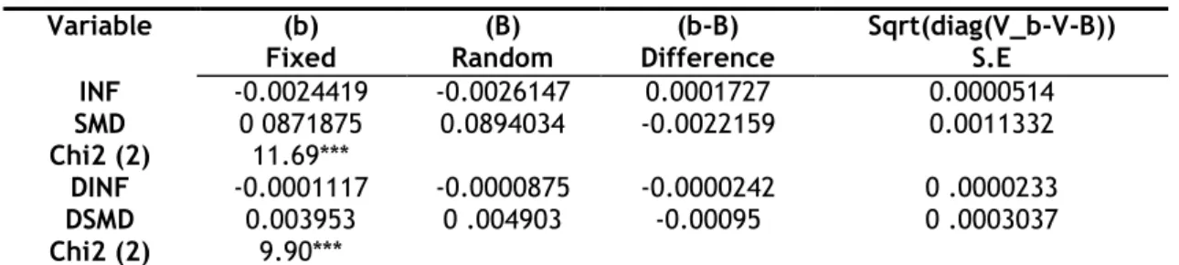
Table 5: Hausman TestVariable (b) Fixed (B) Random (b-B) Difference Sqrt(diag(V_b-V-B)) S.E INF -0.0024419 -0.0026147 0.0001727 0.0000514 SMD 0 0871875 0.0894034 -0.0022159 0.0011332 Chi2 (2) 11.69*** DINF -0.0001117 -0.0000875 -0.0000242 0 .0000233 DSMD 0.003953 0 .004903 -0.00095 0 .0003037 Chi2 (2) 9.90***
Notes: *** denotes statistical significance level of 1% .
The null hypothesis of the Hausman test is difference in coefficients not systematic, in our case the result indicates that our model is a fixed effects model (p-value< 0.05). The following step was to calculate the lag-order selection statistics by following (Grossmann et al., 2014) procedure. This procedure computes the overall coefficient of determination (CD), Hansen´s J statistic (J) and its p- value (J p-value), also was computed the MBIC, MAIC and MQIC that are tree model selection criteria by Andrews and Lu (2001). Was used a maximum of four lags totalizing 279 observations, 31 panels and an average of number T of 9. Table 6 reveals the results.
Table 6: Lag order selection on estimation
Lag CD J J pvalue MBIC MAIC MQIC
1 0.8072152 50.08506 0.004449 -101.9577 -3.914939 -43.24447 2 0.8551336 19.22595 0.3780355 -82.13586 -16.77405 -42.99374 3 0.8530872 13.3973 0.1454375 -37.28361 -4.602702 -17.71255 4 0.7314111
Notes: Stata the command pvarsoc was used.
Once MBIC and MQIC values are lower at one lag, so was selected a first-order PVAR. In a small sample size like ours, the use of two lags sacrifices too much degrees of freedom.
8
4. Empirical Results
A PVAR was estimate using one lag and due the fact that was used variables in their first differences. Was used the option gmmstyle (in the pvar command) that replace missing values with zero (Holtz-Eakin et al., 1988). The results are showed in Table 7. Following this procedure was enlarged the number of observations, what results in a more efficient results. The Granger causality test, using Wald test for each equation of the PVAR, was (see Table 8)
Table 7 : VAR model Results Response of Response to DLGDPpc DINF DSMD DLGDPpc 0.1650197(2.41)** 0 .0007363(2.20)** 0.031929(9.08)*** DINF 65.45823(3.07)*** -0.4938517(-5.16)*** 5.021746(3.93)*** DSMD -2.858854(-2.60)*** -0.003063(-0.87) -0.3199613(-5.85)*** N obs 372 N panels 31
Notes: the regression coefficients are shown in first place; inside parentheses are the heteroscedasticity adjusted t-statistics; *** and **denote statistical significance level of 1% and 5%, respectively; the Stata command pvar. With the option GMM, with one lag, was used.
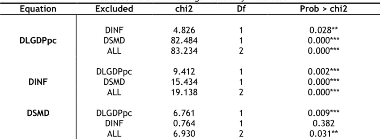
Table 8: Panel VAR-Granger causality Wald test
Equation Excluded chi2 Df Prob > chi2
DLGDPpc DINF 4.826 1 0.028** DSMD 82.484 1 0.000*** ALL 83.234 2 0.000*** DINF DLGDPpc DSMD 15.434 9.412 1 1 0.002*** 0.000*** ALL 19.138 2 0.000*** DSMD DLGDPpc 6.761 1 0.009*** DINF 0.764 1 0.382 ALL 6.930 2 0.031**
Notes: *** and ** denotes statistical significance level of 1% and 5% respectively; the Stata command
pvargranger was used.
The Panel VAR-Granger causality Wald test, shows the presence of a bi-directional causality between economic growth and inflation, and also between economic growth and Stock market development. There is a unidirectional causality between Stock market development and inflation.
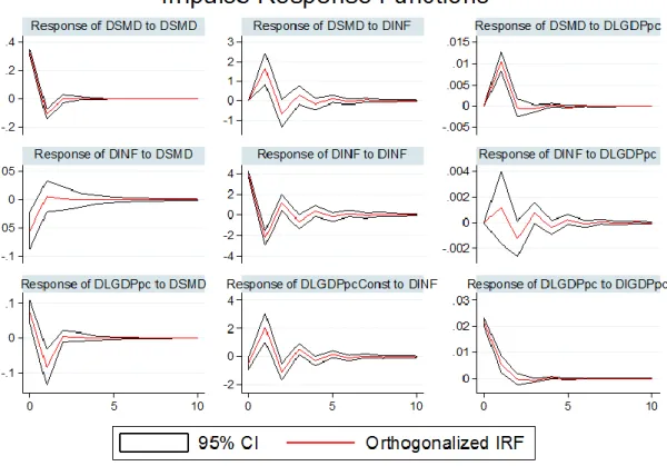
Figure 1 shows the simulations of impulse response functions, were is possible to observe the behaviour of row variables to an existing impulse in the column variables. The 5th and the 95th percentile error bands, in graphics represented by black lines, were estimated by Monte Carlo with 1000 repetitions
9
Figure 1. Impulse-Response FunctionsIn Figure 1 is possible to observe that all the variables return to zero, after a shock, in maximum of five years. This behavior means that variables are stationary, what is consistence with the results previous obtained. A one standard deviation shock to DSMD causes a negative response by DINF. Introducing a deviation shock to DINF, all variables return to the equilibrium after 5 periods. The impact of the shock of INF in DLGDPpc is higher that the shock of INF in DSMD. A deviation shock in DLGDPpc causes a positive impact on DINF and DSMD, but DSMD and DINF returns to the equilibrium after two and five periods, respectively. This results are in line with the literature, this system is a reactive system that after a few periods all variables return to the equilibrium by a harmonic movement.
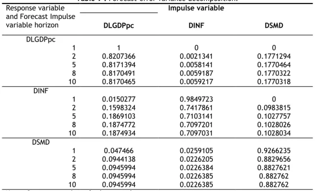
Forecast-error variance decomposition (Table 9) represents how a variable respond to shocks in specific variables (Marques et al., 2013).
10
Table 9 : Forecast-error variance decomposition.Response variable and Forecast Impulse variable horizon Impulse variable DLGDPpc DINF DSMD DLGDPpc 1 1 0 0 2 0.8207366 0.0021341 0.1771294 5 0.8171394 0.0058141 0.1770464 8 0.8170491 0.0059187 0.1770322 10 0.8170465 0.0059217 0.1770318 DINF 1 0.0150277 0.9849723 0 2 0.1598324 0.7417861 0.0983815 5 0.1869103 0.7103141 0.1027757 8 0.1874772 0.7097201 0.1028026 10 0.1874934 0.7097031 0.1028034 DSMD 1 0.047466 0.0259105 0.9266235 2 0.0944138 0.0226205 0.8829656 5 0.0945994 0.0226384 0.8827621 8 0.0945994 0.0226385 0.882762 10 0.0945994 0.0226385 0.882762
Notes: Stata command pvarfevd, was used.
The results on Table 9 are consistence with the results from exogeneity tests (see Table 5 and Fig. 1). With regard to DLGDPpc, after a two-year period, shocks to DLGDPpc explain about 82% of the forecast error variance and after 10 years it stabilizes at 81.7%. Analysing the shocks to DINF and DSMD, the shocks to DSMD explains 17.7% and the shocks to DINF explains 0.6% of the forecast variance. Considering DINF in a year period shocks to DINF explains 98.5% of the forecast error variance and after a 10 year-period this percentage reduce to 70.97% while DLGDPpc explains 18.75% and DSMS explains 10.28%. When analysing the impacts on DSMS, a shock on DSMD explains 92.67%% of the forecast error variance after one year and 88.28% after a 10-year period. DLGDPpc and DINF explain 9.46% and 2.26% respectively. The variable DSMD is more autonomous, being almost autoregressive due the fact that auto explains in 88% and the remaining variables have a low impact on DSMD. The adjustment is more dependent of real variables, like DLGDPpc, than the variables of risk, Inflation, because of the safe mechanisms existence in the financial sector.
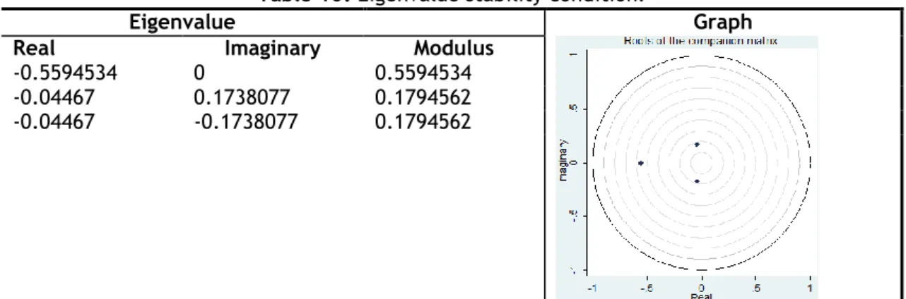
To check the robust of the PVAR was performance a stability test This command tests the condition of eigenvalue. The Table 9 shows the results and the graph of eigenvalues.
11
Table 10: Eigenvalue stability condition.Eigenvalue Graph
Real Imaginary Modulus
-0.5594534 0 0.5594534
-0.04467 0.1738077 0.1794562 -0.04467 -0.1738077 0.1794562
All the eigenvalues are inside the unit circle meaning PVAR satisfies stability condition; Stata command pvarstable was used.
The eigenvalue stability conditiongraph show that all the eigenvalues are inside the unit circle, confirming that the estimate PVAR is stable (Hamilton 1994; Lutkephol 2005).
12
5. Conclusion
This paper applies a PVAR model, Granger test, impulse response functions and forecast-error variance decomposition to study the relationship between economic growth, inflation and stock market development for 31 countries from 2000 to 2014. Stock market development was measure using a composite variable, performed by PCA method, and economic growth was measure using real gross domestic product was a proxy. Results showed the presence of a bidirectional causality between economic growth and inflation, and between economic growth and stock market development, supporting the feedback hypothesis. There is also a unidirectional causality between Stock market development and inflation, supporting the. supply-leading hypothesis. The found results are in concordance with the literature, strengthening that stock market development plays an important role on countries’ economy.