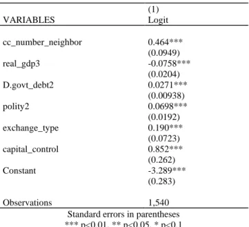
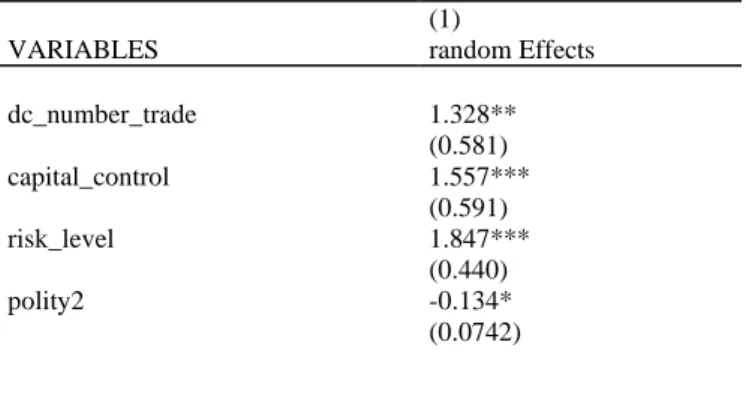
Contagion of financial crises across neighbors and trade partners
127
0
0
Texto
(2)
(3)
(4)
(5)
(6)
(7)
(8)
(9)
(10)
(11)
(12)
(13)
(14)
(15)
(16)
(17)
(18)
(19)
(20)
(21)
(22)
(23)
(24)
(25)
(26)
(27)
(28)
(29)
(30)
Imagem


+7


Documentos relacionados
Tiver profissionais adequados e competentes Tiver profissionais competentes llll Tiver profissionais adequados e competentes Tiver bons funcionários ll Tiver
Com este trabalho pretendeu-se caracterizar a população com alta hospi- talar na região de Lisboa e Vale do Tejo entre 2009 e 2011, com mais de 1 dia e menos de 365 dias
França e do “que poderíamos chamar a sua escola” sobre o caso do surrealismo português, mas também a tripartição do modernismo português “…considerando que, tal
Acerca do surgimento do direito fundamental à vida privada: Pode-se dizer que ele somente veio a ser apercebido como uma das projeções da dignidade da pessoa humana quando
Durante vários anos foram estudados certos padrões comportamentais com possível risco para o desenvolvimento de ITUs recorrentes, tais como micção pré e pós-coital, frequência
Wilson Henry Irvine, nascido no Nordeste dos EUA no ano de 1869 e falecido na mesma região em 1936, foi um mestre do paisagismo no Impressionismo americano
O presente trabalho objetivou quantificar MLT, trans-RSV, fenólicos totais e a atividade antioxidante (AA) em vinhos monocasta portugueses, bem como averiguar a
A análise do contexto pretende caracterizar o ambiente em que decorreram as atividades ou ações planeadas no projeto de intervenção, dotar os recursos disponíveis e/ou necessários à
