THE MARGINS OF PORTUGUESE TRADE AND THE EURO

Universidade Técnica de Lisboa

Instituto Superior de Economia e Gestão

Master in Applied Econometrics and Forecasting

2010/2011

THE MARGINS OF PORTUGUESE TRADE AND THE EURO

Author Advisor

Wilson Nicolau Melim Araújo Luca David Opromolla

ABSTRACT

By Wilson M. Araújo

This paper analyzes the cross-sectional and time-series characteristics of

Portuguese exports between 1995 and 2002, before and after the introduction of

the single European currency – the Euro. The analysis focuses on a set of trade

margins, that compose the total value of exports in a given market, including the

number of exporting firms, the number of products exported (extensive margin),

and the average exports per firm-product pair (intensive margin).

Using an extremely rich and comprehensive international trade data set for

Portugal, we show the following results. First, the extensive margin (mainly the

number of exporters and the number of exported products) is the main factor

explaining the cross-sectional variation of Portuguese exports across trading

partners. Second, the evolution over time of all trade margins for the Euro Zone is

dominated by a unit root, implying, for example, that shocks affecting the number

of exporters, the number of exported products or the average exports per

firm-product pair will have permanent effects. Third, we identify three potential effects

of the introduction of the Euro in 1999: (i) a positive effect on the number of

exporting firms in the four years before the introduction; (ii) a positive effect on

the intensive margin, i.e. average exports per firm-product pair, from 1998 until

2002, and (iii) a tendency for firms to homogenize the set of products exported to

RESUMO

Por Wilson M. Araújo

Este artigo analisa as características seccionais e temporais das exportações

Portuguesas entre 1995 e 2002, antes e depois da introdução da moeda única

europeia - o Euro. A análise baseia-se num conjunto de margens de comércio, que

compõem o valor total das exportações num dado mercado, incluindo o número

de empresas exportadoras, o número de produtos exportados (margem extensiva),

e as exportações médias por combinação empresa-produto (margem intensiva).

Usando uma base de dados de comércio internacional para Portugal,

extremamente rica e extensiva, demonstramos os seguintes resultados. Em

primeiro lugar, a margem extensiva (principalmente o número de exportadores e o

número de produtos exportados) é o principal factor que explica a variação

seccional das exportações Portuguesas entre os parceiros comerciais. Em segundo

lugar, a evolução ao longo do tempo de todas as margens de comércio para a Zona

Euro é dominada por uma raiz unitária, implicando, por exemplo, que os choques

que afectam o número de exportadores, o número de produtos exportados ou as

exportações médias por combinação empresa-produto terão efeitos permanentes.

Em terceiro lugar, identificamos três possíveis efeitos da introdução do Euro em

1999: (i) um efeito positivo sobre o número de empresas exportadoras nos quatro

anos anteriores à introdução, (ii) um efeito positivo na margem intensiva, i.e.,

uma tendência para as empresas homogeneizarem o conjunto de produtos

ACKNOWLEDGMENTS

I would like to thank the economists of the Research Department of the

Bank of Portugal, and especially my advisor Luca David Opromolla for their very

important suggestions, continuing support and motivation. I also would like to

thank Mário Centeno for his comprehension, and Paulo Rodrigues for his help in

opening up new research paths.

I could not forget my family as well. They were always by my side in the

good and the bad moments. I am very grateful to them.

Last but not least, a great thank you to Cláudia Barradas who worked with

me at the beginning of this long journey.

Thanks to you all.

CONTENTS

1. Introduction ... 1 

2. Short Review of the Relevant Literature ... 3 

3. Data ... 5 

3.1. Trade Data ... 5 

3.2. Other Data Sources ... 7 

3.3. A First Glance to Portuguese Exports ... 7 

4. Empirical Methodology ... 8 

4.1. Decomposing Aggregate Exports into Extensive and Intensive Margins .... 9 

4.2. Cross-Sectional Variation in Total Exports ... 10 

4.3. Trade Margins over Time ... 11 

4.3.1. Stationary or Unit-Root Processes and Trade Margins ... 11 

4.3.2. Unit-Root Test on Trade Margins ... 13 

4.4. Euro Effects on Trade Margins ... 18 

5. Empirical Results ... 22 

5.1. Cross-Sectional Variation in Total Exports ... 22 

5.2. Unit-Root Test on Trade Margins ... 23 

5.3. Euro Effects on Trade Margins ... 25 

6. Conclusions ... 27 

References ... 29 

Appendix A – Figures ... 32 

Appendix B – Tables ... 35 

LIST OF FIGURES

Figure 1 – Evolution of Portuguese Exports, 1995-2002 ... 32 

Figure 2 – Evolution of the Portuguese Trade Margins, 1995-2002 ... 33 

LIST OF TABLES

Table I – Sample of Countries used in the Empirical Investigation ... 35 

Table II – Summary Statistics, Portugal, 1999 ... 36 

Table III – Growth Rates of Portuguese Exports (%) ... 36 

Table IV – OLS Regression Decomposition of Portuguese Exports across Trading Partners, 1995-2002 ... 37 

Table V – Unit-Root Test on Trade Margins ... 39 

Table VI – Euro Effects Constant over Time ... 40 

1. INTRODUCTION

The great majority of the recent theoretical and empirical contributions to

the economics literature on international trade have been characterized by an

increasing attention to the role played by firms. The decision of entering or exiting

a foreign market, the decision of which products to export, and the actual sales per

firm-product are problems and outcomes that have gone under more and more

intense scrutiny. In other words, the division of trade into an intensive and an

extensive margin has become standard and it is justified by the fact that not only

the “intensity with which firms trade” matters, but also “how they trade”. The

analysis of trade margins helps explaining the evolution of aggregate trade flows

between countries, and understanding how aggregate trade flows respond to

external shocks.

One of the most important economic events in history occurred in 1999 with

the introduction of the Euro in eleven European countries.1 The introduction of a single currency was expected to reduce the (variable and fixed) costs of trade, and

allow individuals and businesses to make exchanges that were previously

unprofitable. Therefore, the Euro was expected to promote welfare through the

facilitation of trade within the Euro Area.

Despite the fact that more than ten years have passed since the introduction

of the Euro and the existence of several studies on its impacts on trade, the lack of

country-specific evidence on trade margins is still considerable. This paper fills

1

this gap by decomposing Portuguese aggregate exports into trade margins and

studying their characteristics before and after the introduction of the Euro.

Using an extremely rich and extensive international trade data set for

Portugal, this paper analyzes the exports margins between 1995 and 2002.

Portuguese aggregate exports to a given destination are decomposed into four

components, as in Bernard et al. (2009): the number of exporting firms, the

number of products exported, the average exports per firm-product, and a residual

term (the density) capturing the degree of homogeneity in the set of products

exported across destinations. The intensive margin is captured by the third term,

while the extensive margin is composed by the other three terms.

Employing the above decomposition, we make three main contributions to

the literature. First, we take a cross-sectional approach and quantify the

importance of each margin in explaining the variation of exports across Euro Zone

and non-Euro Zone trading partners. Second, we adopt a time-series approach and

test for the presence of a unit root in each of the four trade margins. This allows us

to identify whether the evolution of the trade margins for the Euro Zone is well

described by a stationary or by a unit-root process. An important aspect of our

analysis is that it employs a unit-root test that allows for the presence of an

unknown number of nonlinear breaks in the deterministic component of each

trade margins series. Finally, we provide some initial evidence on the causal

impact of the introduction of the Euro on trade margins. To this end, we estimate

difference-in-differences approach, while in the second we allow for time varying

treatment effects.

Several results emerge from the analysis. First, we find that variation in

exports across trading partners is mainly governed by the extensive margin.

Second, unit-root tests suggest the existence of a unit root in all margins series.

Third, using a difference-in-differences approach we estimate a positive

instantaneous impact of the Euro on the density and on the average exports, a

negative impact on the number of products exported, and no significant effect on

the number of exporting firms. When allowing for time-varying treatment effects,

we estimate significant positive effects (i) on the number of exporting firms in the

four years preceding the actual introduction of the Euro, and (ii) on both average

exports per firm-product and density in the four years following the introduction

of the Euro.

The remainder of the paper is organized as follows. Section 2 provides a

short review of the relevant literature, while Section 3 describes the data used in

the empirical investigation. Sections 4 and 5 present the empirical methodology

and the results, respectively, and Section 6 concludes.

2. SHORT REVIEW OF THE RELEVANT LITERATURE

The study of trade margins plays a key role in international trade. The

possibility of dissecting trade data along the firm, product, and country

dimensions has allowed researchers to gain important insights in understanding

customary to talk about extensive and intensive margins of trade. The extensive

margin is the one that has undergone several changes in its composition. Initially,

the study of the extensive margin only contemplated the product margin, such as

the goods specialization, but over the years, more particularly after the nineties,

the firm margin began to conquer its space so that recent investigation in

international trade consider it now fundamental for understanding general patterns

of trade. While the first models mentioning firms, such as Krugman (1980)

considered that either all or no firms took part in trade, more recent models like

Melitz (2003) consider that firms are heterogeneous, though mono-product

exporters. To overcome this weakness of heterogeneous-firm models, some

modifications have been introduced, in which firms are allowed to export more

than a single product on each market. Trade models as those in Bernard et al.

(2006) or Eckel & Neary (2006) encompass this assumption. As a consequence,

these last developments legitimated the emergence of new extensive margins as

the number of products exported per firm and the number of firm-product

combinations exported to a given destination.

In spite of the recent advances in the theory of international trade, there are

only few studies that analyse the impact of the adoption of the Euro on

intra-European trade taking advantage of firm-level or more disaggregated data sets.

Baldwin & Nino (2006) and Flam & Nordström (2006) use a bilateral trade data

set at the product-level and find evidence that the effects of the Euro on trade

manifest themselves mainly through the variation in the number of product

adoption of the Euro, Berthou & Fontagné (2008) makes use of French firm-level

export data and a business survey to conclude that there is a positive impact of the

Euro on firms’ decisions to export, on the number of products exported and on the

export value per product, for larger and more productive manufacturing firms.

Baldwin et al. (2008) uses the same kind of firm-level data for Belgium, France

and Hungary. They compute a set of descriptive statistics that show an increase in

the number of products exported by French firms to Euro Zone countries in 1999,

compared to other destinations. Analogous conclusions were drawn from the

number of destinations per product per firm for Belgian and French cases.

3. DATA

This section describes the data used in the empirical investigation. In

addition, the last subsection provides a brief analysis of the evolution of

Portuguese exports over time.

3.1. Trade Data

The trade data set employed in this thesis was provided by Statistics

Portugal (Instituto Nacional de Estatística – INE). It contains information on all

export and import transactions made by Portuguese mainland-based firms during

the period from 1995 to 2005. Each data point includes information on the year

and month of the transaction, the firm’s identifier, the product code (an eight-digit

transacted (in kilos), the (nominal) value of the transaction in Euros, the transport

mode, the relevant international commercial term (CIF, FOB, etc.) among others.2

One of the most important features of this data set is that it allows drawing

information on how many firms and products are involved in trade relationships

with a given country at any moment in time. The sample used in this study covers

the period 1995-2002 and 27 destinations.

The reasons behind the choice of the time horizon, 1995-2002, are the

following: avoiding complications related to the EU enlargement in 2004 and

studying the evolution of exports in a period that covers the 4 years immediately

preceding and following the introduction of the Euro. Destinations are divided

into two groups: nine Euro Zone countries, that compose the treatment group in

the difference-in-difference analysis, and 18 OECD (Organization for Economic

Co-operation and Development) non-Euro Zone countries, that represent the

control group in the difference-in-difference analysis.3 Table I in Appendix B reports the countries used in the empirical investigation, distinguishing them by

Euro Zone (9 countries) and non-Euro Zone (18 countries).4

2

The Combined Nomenclature (CN) is a system that defines the general rules for the classification of commodities, imported into or exported from the European Union, to an eight-digit code and is adjusted on a yearly basis. This system is composed of the Harmonized System (HS) with additional European Community subdivisions: the first six digits of the CN roughly coincide with the HS classification. The HS classification is run by the World Customs Organization and is widely used in international trade relationships.

3

Note that these 27 destinations represent about 91% of Portuguese exports over the period 1995-2002.

4

3.2. Other Data Sources

In order to enrich the econometric analysis in the difference-in-differences

approach, the respective estimations also include the real GDP of the destination

and the bilateral real exchange rate as covariates. Information on (real and

nominal) gross domestic product and bilateral nominal exchange rates were

obtained from OECD and Bank of Portugal websites, respectively. With this

information, the bilateral real exchange rates were constructed based on the GDP

deflators, in Euros.

3.3. A First Glance to Portuguese Exports

An initial analysis on Portuguese exports and some of their components

helps to identify different behaviour patterns, before and after the introduction of

the Euro and between Euro Zone and non-Euro Zone.

Table II in Appendix B shows some descriptive statistics of Portuguese

exports, in 1999. The numbers indicate that Portugal was more active, in all

respects, within the Euro Zone than outside in the year when the Euro was

introduced. This pattern is to be expected if we think that the Euro considerably

reduced trade costs within the Euro Zone. However, as we will see below, the

evolution of these indicators over time makes this interpretation less

straightforward.

Figure 1 in Appendix A displays the evolution of the annual series: export

value, number of exporting firms, number of product categories exported and

2002. Table III in Appendix B contains, for each series, the respective

1995-1998 and 1999-2002 growth rates.

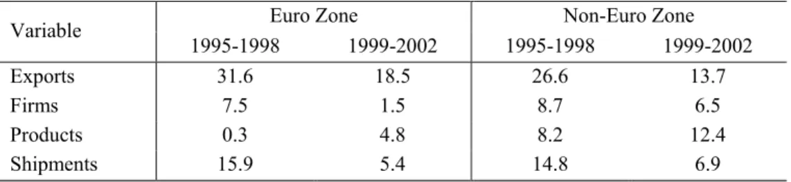
Three main patterns stand out from Table III: (i) the series on the value of

exports is the one showing the highest growth rates (for the two destinations and

periods considered); (ii) all series except the one on products present superior

growth rates in the pre-Euro period than in the post-Euro period; (iii) with the

exception of the exports value, all post-Euro growth rates are considerably higher

for non-Euro Zone series than for Euro Zone series.

In view of this, apparently there are reasons to argue against the possible

trade creation from Euro introduction: growth rates are higher in pre-Euro period

than the post-Euro period with the single exception of the products exported.

However, it must be clear that from this preliminary analysis it is not possible to

see specific-country evolution (we only see two groups of countries viewed each

one as a single destination) and that might mitigate potential Euro effects at

destination country level. In addition, we need to control for other factors that

may influence trade to estimate, if present, the Euro effects.

4. EMPIRICAL METHODOLOGY

This section provides the econometric methodology applied in the empirical

investigation and that is based in a decomposition of Portuguese exports into four

4.1. Decomposing Aggregate Exports into Extensive and Intensive Margins

As discussed above, the analysis focuses on four components of the value of

Portuguese exports to a given destination. Following Bernard et al. (2009),

Portuguese exports to destination i (xti) can be decomposed into the product of the

number of firms exporting to that destination (fi), the number of product

categories exported to the destination (pi), the density of trade (di) (to be defined

below), and the average value of exports per firm-product (xi),

(1) xt_i = f p d x_{i i i i},

where / (d_i=o_i f p_{i i}), oi is the number of firm-product pairs for which exports to

destination i are positive and x_i =xt o_i/ _i. In this decomposition the extensive

margin is captured by the first three margins (fi, pi and di), while the intensive

margin is present through the last term xi. It is important to include the density

term in order to adjust for the fact that not all firms trade all products. If firms

tend to export a constant set of product categories, Bernard et al. (2009) alert that

density is negatively correlated with the number of exporting firms and products

exported:

As the number of firms and products grows across countries, the

number of possible firm-product observations (fi pi) expands

multiplicatively. If firms are active in a relatively constant

firm-product observations with positive trade will expand less than

proportionately, causing density to decline.

In Bernard et al. (2009), p. 4.

Next subsections include the econometric methodology adopted in this

paper in order to concretize the empirical investigation.

4.2. Cross-Sectional Variation in Total Exports

Whether the extensive or the intensive margin contributes most to

differences in exports across trading partners is a question that recently gained

considerable attention in the international trade literature. In this section, we

describe the methodology used to analyze the contribution of each margin to

explain the differences in Portuguese exports across trading partners for a given

year.

The methodology that we adopt was introduced in Bernard et al. (2009).

Using the decomposition of Portuguese exports in equation (1) we regress the

logarithm of each margin (firms, products, density, and average exports) on a

constant and on the logarithm of total exports using ordinary least squares. Let yi

represents one of the four trade margins to destination i, i.e., y_iÎ

{

}

then the four regressions to be estimated for each year are:

where uy,i is the error term when the dependent variable is the logarithm of the

trade margin y, cy is a constant and βy is the parameter of interest and represents

the share of the whole variation in exports explained by margin y. Noting that the

decomposition in (1) is log-linear and knowing that OLS is a linear estimator with

zero mean residuals, the sum of the estimated coefficients ˆβ_y from the four

equations is equal to unity, i.e., ˆβ β β β_f + ˆ_p+ + =ˆ_d ˆ_x 1.5 Finally, in order to find differences in margins’ contributions across trading partners, the four regressions

are estimated for three different groups of destination countries: OECD countries

(n=27) and within OECD, Euro Zone countries (n=9) and non-Euro Zone

countries (n=18).

4.3. Trade Margins over Time

This part assesses the evolution of the trade margins over time. After a small

introduction about the distinction between stationary and unit-root processes, we

describe the methodology used to test for the presence of a unit root in the trade

margins time series.

4.3.1. Stationary or Unit-Root Processes and Trade Margins

Amongst several important subjects around macroeconomics, the evolution

of economic series over time when these display an increasing trend (such as

exports) remains a striking object of study. An important question that continues

to deserve a lot of attention in this respect is to know whether a time series is

5

stationary or not. In other words, are series better approximated by a I(0) or a I(1)

process? The answer to this question is of particular interest because the

understanding of how exports behave over time has huge implications on the role

of the economic policy. If the series is I(1) (contains a unit root), then the shocks

affecting the series will have permanent effects on the series level and policy

action is required to return series to its original level. On the other hand, if the

series is I(0), the shocks affecting the series will purely be transitory, and, in this

case, the need for policy action is less obligatory because the series will

eventually return to its equilibrium level.

Once trade margins and the introduction of the Euro are central in this

study, we test for the presence of a unit root on Portuguese trade margins series

for the Euro Zone. To make possible the application of these tests, the trade

margins time series were constructed from equation (1) on a monthly basis

(between 1995 and 2002) and considering Euro Zone as a single destination.

Figure 2 in Appendix A shows the evolution over the period 1995-2002 of the

respective monthly trade margins series. As we can see, all series display

seasonality and an increasing trend over time, except density which exhibits a

decreasing trend. A decreasing trend for the density series is to be expected since,

as explained above, density is negatively correlated with the number of firms and

products, both increasing over time.

Below we present the methodology used to check for non-stationarity of the

trade margins time-series. Our methodology is based on the well-known

modification on its usual specification is introduced in order to safeguard results

when there are potential structural breaks in series as those related to the

introduction of the Euro. If the presence of a unit root is not rejected the series

seems well approximated by a I(1) process, while a I(0) process seems more

adequate when the presence of a unit root is rejected.

4.3.2. Unit-Root Test on Trade Margins

The traditional DF tests are very popular amongst unit-root tests. However,

since Perron’s (1989) seminal paper, it is known that ignoring the existence of

structural breaks in a series has very problematic consequences for these tests,

mainly the loss of power and size distortion. An alternative method to consider

breaks that was initially proposed was to approximate the breaks using dummy

variables. This method turned out to have several drawbacks: (i) it is necessary to

know the exact number and location of the breaks which are almost always

unknown; (ii) the tests accounted only for one or two breaks, which is very

restrictive; (iii) the use of dummy variables suggests sharp changes in the trend or

level; since breaks in economic series often gradually display their impacts over

time, dummies will not capture well this behaviour. The latter drawback is

particularly relevant in the context of this study since it is likely that the

introduction of the Euro displayed its effects only gradually over time. Recent

developments in unit-root tests allow us to overcome the above difficulties.

Below, we will test for a unit root in the presence of structural breaks using an

equally well, i.e. it has good size and power properties, both in the presence of

gradual and sharp breaks.

Enders & Lee (2009) modifies the usual DF test implementing a variant of

the Flexible Fourier transform (see Gallant (1981)) to control for the unknown

nature of the breaks. A Fourier adjustment, using only a small number of low

frequency components, is able to capture the types of breaks that we usually see in

economic data. We take this approach to account for breaks because it is

reasonable to think that the effects of the introduction of the Euro were spread out

over time and did not fully manifest themselves in 1999. Therefore, the usual DF

specification will also include a time-dependent deterministic term α(t):

(3) y_t =α( )t + +γt δy_t-1+ε_t,

where α(t) can be written as:

(4) ₀

1 1

( ) sin(2 / ) cos(2 / ), / 2

n n

k k

k k

α t α α πkt T β πkt T n T

= =

= +

å

å

In the above formulation ((3) and (4) altogether), ε_t is a stationary error term with

variance 2

ε

σ , n is the total number of frequencies contained in the Fourier

adjustment, k is a particular frequency and T is the number of observations.

Following Enders & Lee (2009) that a single frequency k can capture an ample

variety of breaks that we see in economic data, the resulting equation, from (3)

and (4), is:

or equivalently:

(6) ∆y_t = +µ αsin(2πkt T/ )+βcos(2πkt T/ )+ +ηt fy_t-1+e_t,

where yt-1 was subtracted on both sides of (5) such that fº -θ 1. This last

expression (6) is very useful since it allows testing for a unit root directly from the

t-ratio of f. As residuals might display serial correlation, (6) is augmented with

lagged values of ∆yt:

(7) _{0 1 2 3 1}

1

∆ sin(2 / ) cos(2 / ) ∆

l

t t i t i t

i

y b b πkt T b πkt T b t ρy_- λ y_- u

=

= + + + + +

å

In order to determine the lag length l we follow the GTS t-sig strategy, consisting

of a t-test at 10% significance level on the last augmented term until reject the null

of λl = 0.6 At the same time, when it is possible to eliminate the last lag, serial

correlation tests on residuals are implemented to verify if the elimination of the

last augmented term caused serial correlation; if it did, then the term is not

excluded and that is the equation test for a unit root.7 To choose the maximum of l to start with, it is used the l12 rule present in Schwert (1989):

1/ 4

max( ) 12.( / 100)

l T = ëé T ù_û, where [.] represents “the integer part of”. But, since this

rule is not suited to maximize the power of the test, it is used a “smoothed”

version: as the total number of observations of margins series is T = 96, according

to l12 rule the lmax is 11; then it is set lmax=10.

6

GTS t-sig stands for “general-to-specific sequential t-sig”. This method is described in Lopes (2010).

7

Finally, the hypothesis test for a unit root is simply:

(8) H₀:ρ=0 vs H₁:ρ<0

on (7) using τ_DF =ρˆ/se( )ρˆ . The critical values for this test are reported in Enders

& Lee (2009).

However, as we have seen, this method depends on the value of the

frequency k, and because this is generally unknown, it needs to be estimated in

first place. A grid-search procedure that consistently estimates k is to estimate

equation (6) for each integer k = 1, 2, ..., 5. ˆk results from the regression with the

smallest “Sum Squared of Residuals” (SSR). As such, the unit-root test is applied

on (7) with ˆk.

Now, we already know how to proceed in the case of a structural break on a

series. And what if there is no need to account for structural breaks? In this case,

Enders & Lee (2009) recommend performing the usual linear DF test without the

trigonometric terms because it will have more power. As wee clearly see, the

“standard” DF test emerges as a special case of (6) making α= β= 0. Enders &

Lee (2009) also developed an F-test for the null α= β= 0, using the following F

-statistic:

(9) 0 1

1

( ( )) / 2

( )

( ) / ( )

SSR SSR k

F k

SSR k T q

-=

- ,

where SSR1(k) is the SSR from (6), SSR0 is the SSR from the regression without

observations. But, since k needs to be estimated, they consider the following

modification of the F-test in (9):

(10) ( )ˆ max ( ) k

F k = F k ,

where kˆ=arg max ( )k F k . As it is evident, the ˆk giving the smallest SSR value

will maximize the F-statistic in (9) such that kˆ=arg inf SSR ( )k ₁ k . They report

the critical values for this test in their paper. If the sample value of F k( )ˆ is larger

than the respective critical value, the test for a unit root uses equation (7) with the

trigonometric terms. On the contrary, if the null is not rejected, then it is possible

to augment power by using the usual linear DF test (equation (7) without the

trigonometric terms).

Below, we summarize in three steps the methodology presented in this part

and that is applied on Portuguese trade margins series for the Euro Zone. As series

were collected monthly and they display seasonality, all regressions mentioned

below also include the usual eleven monthly dummies to account for it. Therefore,

considering yt as a trade margin, the procedure is as follows:

Step 1: Estimate (6) for integer values of k from 1 to 5. ˆk _{results from the}

regression with the smallest SSR.

Step 2: Perform the F-test for a break (α= β= 0) on equation (6) with ˆk , using

(9). If the null α= β= 0 is rejected, use (7) to test for a unit root. If the null is not

Step 3: Test for a unit root using (7) with or without the trigonometric terms. In

any case, the hypothesis test for a unit root is the same described in (8),

0: 0 1: 0

H ρ= vs H ρ< . If H0 is not rejected, we do not reject the existence of a

unit root and then, the margin series seems well approximated by a I(1) process.

On the contrary, the rejection of H0 implies the rejection of a unit root and thus, a

I(0) process will approximate better the series.

To see how well a Fourier approximation mimics the time path of the

margins series, Figure 3 in Appendix A shows the seasonally adjusted margins

series along with the nonlinear trend Fourier adjustment (dashed lines) obtained

by estimating the regression y_t =c₀ +c₁sin(2πkt Tˆ / )+c₂cos(2πkt Tˆ / )+c t₃ +v_t,

where ˆk results from “Step 1” above. As we can see by the dashed lines, each

series seems particularly well approximated, though this adjustment is not always

necessary.

4.4. Euro Effects on Trade Margins

In this part, we describe the methodology used to identify the impact of the

Euro on Portuguese trade margins. Did the Euro raise the number of Portuguese

exporting firms and the product categories exported? How did export value per

firm-product respond to the introduction of the Euro? These kinds of questions are

central when analyzing currency union effects on trade margins. To explore them

for the Portuguese case, we use a balanced annual panel dataset from 1995 to

we apply a difference-in-differences approach to estimate the Euro effects on the

four Portuguese trade margins.

The difference-in-differences technique measures the effect of a treatment at

a given period in time. The reasoning of this technique consists of examining the

effect of some kind of treatment by comparing the treatment group after treatment

both to the treatment group before treatment and to a control group. Though its

weakness is to incorrectly identify the treatment effect when something else

occurs between the two groups at the same time as treatment, this method is

simple to implement and under certain assumptions is also a strong econometric

tool to evaluate the effects of an important policy. In this study, the treatment

group is composed of the countries that entered the Euro Zone in January 1999 (9

destinations) while the control group is composed of the countries that never

entered the Euro Zone (18 destinations).8 According to this methodology, the key assumptions that permit to identify the effect of the introduction of the Euro on

the trade margins are two: (i) the introduction of the Euro produced a constant

instantaneous effect; (ii) exports to Euro Zone and non-Euro Zone countries

would evolve by the same way in the absence of Euro.

Letting yit be a trade margin to a given destination country i at time t,

{

}

it it it it it

y Î f p d x , the Euro effects on each trade margin are estimated using

the fixed effects Poisson estimator, with robust standard errors clustered by

destination country, on the following gravity equation:

8

(11) y_it =exp

(

)

EZit, the variable of interest inherent with the difference-in-differences method, is

a dummy variable equal to one over the period 1999-2002 when the destination

country is a member of the Euro Zone, and zero otherwise. ln(rgdpit) is the natural

logarithm of the destination’s real gross domestic product. ln(rerit) is the natural

logarithm of the real exchange rate. κ_i and κ_t are the sets of 26 destination and 7

year dummies, respectively, in order to get a fixed effects estimator to deal with

the unobserved heterogeneity. The reason behind the use of the Poisson estimator

is related to the gravity equation generally applied in international trade area. In

this respect, Silva & Tenreyro (2005) argue that taking the logs in a gravity

equation, as in (11), and apply OLS in the presence of heteroskedasticity leads to

biased and inconsistent estimates because, in this case, we would get

ln( ) |_ity _it 0

Eé_ë e x ù¹_û , since “the expected value of the logarithm of a random

variable depends both on its mean and the higher-order moments of the

distribution”. As an alternative, Silva & Tenreyro (2005) suggest applying directly

the Poisson maximum likelihood estimator on (11), where the key assumption that

provides unbiased and consistent estimates of the parameters is that the regressors

are strongly exogenous. Second section of the Appendix C shows this fact.

The traditional gravity models make use of cross-section data on different

pairs of trading partners and include both exporter and importer GDP in the

single exporting country (in this case Portugal), “exporter income is captured in

the regression constant and only importer income is included in the regression.”

In spite of the difference-in-differences specification in (11) is the usual

method to estimate treatment effects, in this particular case of the Euro seems to

be more adequate to assume that the Euro produced effects even before its

introduction, so that firms started to adjust their trade in a proactivity perspective,

and that these effects may vary over time. Accordingly, if the Euro effects are

spread out over years, then a constant instantaneous effect of the Euro may be

misspecified. To hold this, and following Laporte & Windmeijer (2005), we

introduce some flexibility on the analysis by substituting the dummy step variable,

EZit, by annual pulse variables from 1996 to 2002 in (11):

(12) yit =exp

(

11,

)

y y

t t it

γ κ v

+ ,

where the pulse variable EZ96it is equal to one in 1996 when the destination

country belongs (or in this case, will belong) to Euro Zone and so on for the

remain pulse variables (EZ97it, EZ98it, EZ99it, EZ00it, EZ01it and EZ02it,).

Therefore, the coefficient associated with a given pulse variable represents the

5. EMPIRICAL RESULTS

This section exposes the main results obtained from the methodology

described in previous section. The titles in this section match to the titles in the

respective methodology section for easier linking “methodology-results”.

5.1. Cross-Sectional Variation in Total Exports

The contribution of trade margins (firms, products, density, and average

exports) to cross-sectional variation in Portuguese exports across trading partners

in a given year is obtained by the estimation of the equation (2) using OLS. The

results are displayed in Table IV in Appendix B in which is only reported the

estimate of the slope parameters βy. Once the main conclusions do not change

over years, here it will be discussed the results for 2002 (last part of the table).

Each cell corresponds to a different regression based on equation (2) according to

the margin in study and displays the estimated slope coefficient and standard error

(in parentheses) of that regression at a given year. Thus, each column within a

given year sum to unity. In 2002 (last portion of the table), as we can see in the

last element of the column “OECD”, the intensive margin (given by the average

firm-product exports) explains, on average, about 41% of the variation in

Portuguese exports across OECD destinations. Variation in the number of

exporting firms (first element) and the number of products exported (second

element) account for 50.6% and 41.8% of the variation, respectively. The

coefficient for density is negative (-0.332), revealing the negative correlation with

extensive margin accounts for 59.1% of the variation (more than intensive

margin).9 Similar conclusion is extracted for the other two sets of countries in which OECD is divided: extensive margin accounts for the vast majority of the

variation of Portuguese exports to Euro Zone and non-Euro Zone (56.8% and

64.0%, respectively). Besides that, we can also see that the extensive margin is

even more important for non-Euro Zone than Euro Zone destinations. So, it

follows that the extensive margin is the largest contributor to variation of

Portuguese exports across different destinations, but it is less important to explain

variations of Portuguese exports to Euro Zone countries than to non-Euro Zone

countries. The results do not differ substantially for the other years. Thus,

previous finding alert for the fact that the analysis of Portuguese exports must take

into account not only knowledge on the value exported, but also a very deep

knowledge on exporting firms and products exported.

5.2. Unit-Root Test on Trade Margins

This subsection reports the results from the unit-root tests applied on

Portuguese trade margins series for the Euro Zone. Margins series are observed

monthly from 1995 to 2002 (Figure 2 in Appendix A). We follow the three steps

presented in the methodology section above for taking into account potential

smooth breaks in series, caused by the introduction of the Euro.

As mentioned before, given we are in the presence of monthly series, we

must keep in mind that all regressions involved in calculations, and that will be

9

cited below, additionally include eleven monthly dummies to control for

seasonality.

The first step consists on finding the best frequency k. This is done by

estimating (6), for the integers 1£ £k 5, choosing ˆk (the estimated frequency)

from the estimation yielding the lowest “Sum of Squared Residuals”. First portion

(a) of Table V in Appendix B indicates in last column that the best frequency is

one for firms and density, two for products and three for average firm-product

exports.

In the second step, it is applied an F-test for a break to verify whether the

sine and cosine terms will be needed in the DF equation test for a unit root. At this

stage, it is estimated (6) (where k is replaced by ˆk ) with and without the

trigonometric terms. Then, it is computed the F-statistic as in (9) and (10), and

implemented the test for the null of joint nullity of the two parameters associated

with the sine and cosine terms (α = β = 0). The test is performed at 5%

significance level and the critical value is reported in Enders & Lee (2009). The

last column of the middle portion (b) of Table V in Appendix B shows that the

trigonometric terms are needed in the test equation for firms, but not in the

equations for the other margins (products, density and average exports). For the

latters we will use the usual linear DF test since the F-test did not reject the

inexistence of any break in these series.

Finally, in third and last step is performed the unit-root test on each margin

seen by the previous F-test, the DF equation test with the trigonometric terms will

be applied on firms’ series while the usual linear DF test on the other three series:

products, density and average exports. The test is performed at 5% significance

level and the critical value for the nonlinear DF test is reported in Enders & Lee

(2009). The last portion (c) of Table V in Appendix B shows the results for the

unit-root test based on equation (7). The GTS t-sig strategy complemented with

serial correlation tests on residuals set nine lags for firms, products and average

exports and only one for density. As we can observe, all the t-statistics of ρ (τ_DF)

are higher than the critical values reported in the last column. Therefore, the test

suggests that all series contain a unit root in their data generating process, once is

not possible to reject the null of unit root for all cases. Under this situation, it

follows that all Portuguese trade margins for the Euro Zone are well described by

a I(1) process and, thus, exhibit great persistence with a stochastic trend (unit

root). Having said that, it is expected that all fluctuations in margins represent

permanent shifts in trend and, moreover, macroeconomic shocks have a

permanent or long-run effect on series level.

5.3. Euro Effects on Trade Margins

The results concerning the effect of the introduction of the Euro on the

Portuguese trade margins are the subject of this last section. First, we assume that

the effect of the Euro is instantaneous and constant over time by estimating

equation (11) with the fixed effects Poisson estimator. Table VI in Appendix B

column represents a separate regression according to the trade margin used as the

dependent variable. Looking at the first row, we can see that the Euro had no

significant effect only on the number of exporting firms (fit). Concerning the

number of products exported, we estimate a negative impact of the introduction of

the Euro, but not as strong as the positive effects found for the density and

average exports margins. These last two margins were particularly influenced by

the introduction of the Euro.

The previous results are based on a very restrictive assumption, namely that

the Euro is expected to produce constant effects over time and only after its actual

introduction. The validity of this assumption is very questionable, particularly

because nothing prevents economic agents, such as firms, to pre-react to

announced external shocks. Indeed, it is very likely that firms tend to pre-adjust

their exports in order to maximize their benefits from a shock with high

magnitude, such as the introduction of the Euro in the monetary system.

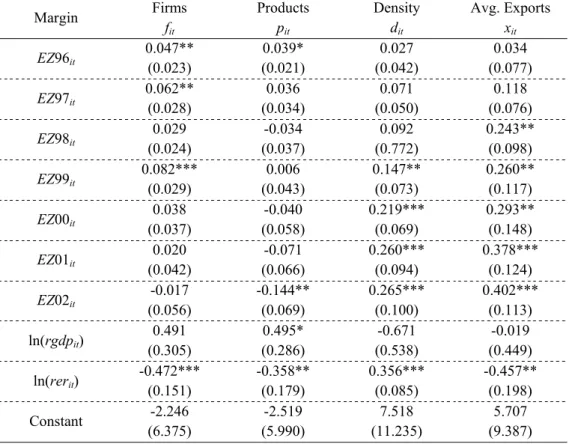
The design of the equation (12) takes the above issues into account. This

specification allows for time varying treatment effects before and after the

introduction of the Euro. The results are now presented in Table VII of the

Appendix B. Two main aspects emerge from the analysis. First, the number of

firms exporting to Euro Zone countries increases in the four years prior to the

actual introduction of the Euro. Second, both average exports per firm-product

and the density terms increase in the four years including and following the

Firms operate under significantly uncertain conditions, constantly making

decisions affecting their costs and productivity. A major source of uncertainty

arises from trade policy, as documented in Handley & Limão (2011). The increase

in the number of firms exporting to Euro Zone destinations, before the actual

introduction of the Euro, reveals an anticipation strategy by firms to create new

business opportunities and to solidify them during that period. However, firms

opted by doing a smooth transition to the new economic reality, as evidenced by

the significant rise of average exports only near Euro introduction. This transition

culminated in the firms’ specialization in more profitable products (reduction of

categories exported), required by the new competition triggered by the “almost”

free trading within Euro Zone after 1999.

6. CONCLUSIONS

The distinction between the extensive and the intensive margins of trade has

recently become central in the field of international trade for understanding the

cross-sectional and time-series determinants of trade, as well as the response of

trade flows to important economic and political events. This paper deals with the

above three issues using detailed information on export transactions conducted by

all firms based in Portugal, over the period 1995-2002.

Results concerning the variation of trade across destination countries show

that these differences are due, in large part, to the extensive margin (the number of

exporting firms, the number of products exported and density) rather than the

We also show that the evolution over time of all trade margins is

characterized by a unit-root. Macroeconomic shocks are therefore expected to

have a permanent effect on the level of trade.

Finally, the last results identify, after 1999, a negative effect of the

introduction of the Euro on the number of products exported, a positive effect on

the density and on the average exports and no significant effect on the number of

exporting firms. Alternatively, if it is assumed that Euro generated effects also

before its introduction, results point out for a positive adjustment on the number

of exporting firms until 1999. The number of products exported display the full

negative impact three years after Euro introduction, in 2002. Density and average

firm-product exports are positively affected by the Euro from 1999 and 1998

onwards, respectively.

This paper is a first attempt in studying the behavior of Portuguese trade

margins in response to important external shocks such as the introduction of the

Euro. Although we provide some initial interesting results, further progress in this

area will require deeper information on firms’ characteristics to identify different

REFERENCES

Baldwin, R. and Nino, V. (2006). Euros and Zeros: The Common Currency Effect

on Trade in New Goods. NBER Working Papers 12673.

Baldwin, R., Fontagné, L., Nino, V., Santis, R. and Taglioni, D. (2008). Study on

the Impact of the Euro on Trade and Investment. European Economy,

Economic Papers 321, May.

Bernard, A., Redding, S. and Schott, P. (2006). Multi-Product Firms and Trade

Liberalization. NBER Working Papers 12782.

Bernard, A., Jensen, J., Redding, S. and Schott, P. (2007). Firms in International

Trade. NBER Working Papers 13054.

Bernard, A., Jensen, J., Redding, S. and Schott, P. (2009). The Margins of US

Trade. American Economic Review: Papers & Proceedings 99 (2), 487-493.

Berthou, A. and Fontagné, L. (2008). The Euro Effects on the Firm and

Product-Level Trade Margins: Evidence from France. CEPII Working Papers

2008-21.

Eckel, C. and Neary, J. (2006). Multi-Product Firms and Flexible Manufacturing

in the Global Economy. CEPR Discussion Papers 5941.

Enders, W. and Lee, J. (2009). The Flexible Fourier Form and Testing for Unit

Department of Economics, Finance and Legal Studies, University of

Alabama.

Flam, H. and Nordström, H. (2006). Euro Effects on the Intensive and Extensive

Margins of Trade. CESifo Working Paper Series 1881.

Gallant, R. (1981). On the Basis in Flexible Functional Form and an Essentially

Unbiased Form: the Flexible Fourier Form. Journal of Econometrics 15,

211-353.

Handley, K. and Limao, N. (2011). Trade and Investment under Policy

Uncertainty: Theory and Firm Evidence. Presented at the 2011 NBER

International Trade and Investment Program Meeting.

Krugman, P. (1980). Scale Economies, Product Differentiation and the Pattern of

Trade. American Economic Review 70, 950-959.

Laporte, A. and Windmeijer, F. (2005). Estimation of Panel Data Models with

Binary Indicators when Treatment Effects are not Constant over Time.

Economics Letters 88 (3), 389-396.

Lopes, A. S. (2010), “Raízes Unitárias – Uma Introdução”, mimeo, ISEG-UTL.

Melitz, M. (2003). The Impact of Trade on Intra-Industry Reallocations and

Aggregate Industry Productivity. Econometrica 71 (6), 1695-1725.

Perron, P. (1989). The Great Crash, the Oil Price Shock, and the Unit Root

Schwert, G. (1989). Tests for Unit Roots: A Monte Carlo Investigation. Journal of

Business and Economic Statistics 2, 147-159.

APPENDIX A – FIGURES

Exports Firms

Products Shipments

Notes: This figure displays the evolution of annual Portuguese exports, and their components, to Euro Zone (EZ – solid lines) and non-Euro Zone (NEZ – dashed lines) destinations over the period 1995-2002. All series are normalized to 100 in 1999.

Figure 1 – Evolution of Portuguese Exports, 1995-2002

1995 1996 1997 1998 1999 2000 2001 2002 75 80 85 90 95 100 105 110 115 120

EZ NEZ

1995 1996 1997 1998 1999 2000 2001 2002 94 96 98 100 102 104

106 EZ NEZ

1995 1996 1997 1998 1999 2000 2001 2002 95.0 97.5 100.0 102.5 105.0 107.5 110.0 112.5

EZ NEZ

1995 1996 1997 1998 1999 2000 2001 2002 85.0 87.5 90.0 92.5 95.0 97.5 100.0 102.5 105.0 107.5

Firms (ft) Products (pt)

Density (dt) Average Exports (xt)

Notes: This figure shows the evolution of monthly series of the Portuguese trade margins, as defined in Section 4.3.1, over the period 1995-2002.

Figure 2 – Evolution of the Portuguese Trade Margins, 1995-2002

1995 1996 1997 1998 1999 2000 2001 2002 2003 3600

3800 4000 4200 4400 4600

Firms

1995 1996 1997 1998 1999 2000 2001 2002 2003 2600

2800 3000 3200 3400 3600

Products

1995 1996 1997 1998 1999 2000 2001 2002 2003 0.000825

0.000850 0.000875 0.000900 0.000925 0.000950 0.000975

0.001000 Density

1995 1996 1997 1998 1999 2000 2001 2002 2003 70000

Firms, s.a. (f’t) Products, s.a. (p’t)

Density, s.a. (d’t) Average Exports, s.a. (x’t)

Notes: This figure displays, for the period 1995-2002, the monthly series of Portuguese trade margins seasonally adjusted (s.a.) (solid lines) and approximated by a nonlinear Fourier trend (dashed lines).

Figure 3 – Fourier Trend Approximation, 1995-2002

1995 1996 1997 1998 1999 2000 2001 2002 2003 3800 3900 4000 4100 4200 4300 4400 4500 4600

Firms_SA Fourier

1995 1996 1997 1998 1999 2000 2001 2002 2003 2800 2900 3000 3100 3200 3300 3400 3500

3600 Products_SA Fourier

1995 1996 1997 1998 1999 2000 2001 2002 2003 0.000825 0.000850 0.000875 0.000900 0.000925 0.000950 0.000975

Density_SA Fourier

1995 1996 1997 1998 1999 2000 2001 2002 2003 70000 75000 80000 85000 90000 95000 100000

APPENDIX B – TABLES

Table I

Sample of Countries used in the Empirical Investigation

Full Sample – 27 OECD Countries

Euro Zone Countries (9) non-Euro Zone Countries (18)

Austria Australia New Zealand

“Belux” Canada Norway

Finland Czech Republic Poland

France Denmark Slovakia

Germany Hungary Sweden

Ireland Iceland Switzerland

Italy Japan Turkey

Netherlands South Korea United Kingdom

Spain Mexico United States

Table II

Summary Statistics, Portugal, 1999

Euro Zone Non-Euro Zone

Number of exporting firms 17,791 14,156

Number of products exported 16,936 13,165

Number of firm-product pairs 61,317 38,862 Avg. Exports per firm-product pair 237.951 137.301 Notes: This table shows some descriptive statistics of Portuguese exports to Euro Zone and non-Euro Zone destinations, in 1999. A product is defined as a distinct eight-digit Combined Nomenclature code. Average exports are expressed in 1999 thousands Euro.

Table III

Growth Rates of Portuguese Exports (%)

Variable Euro Zone Non-Euro Zone

1995-1998 1999-2002 1995-1998 1999-2002

Exports 31.6 18.5 26.6 13.7

Firms 7.5 1.5 8.7 6.5

Table IV

OLS Regression Decomposition of Portuguese Exports across Trading Partners,

1995-2002

Year Margin OECD Euro Zone non-Euro Zone

1995

Firms 0.590*** (0.039)

0.425*** (0.040)

0.639*** (0.057) Products 0.501***

(0.027)

0.439*** (0.058)

0.504*** (0.035) Density -0.388***

(0.031)

-0.308*** (0.054)

-0.404*** (0.042) Avg. Exports 0.297***

(0.035) 0.444*** (0.046) 0.261*** (0.056) 1996

Firms 0.583*** (0.041)

0.450*** (0.043)

0.632*** (0.064) Products 0.505***

(0.031)

0.457*** (0.060)

0.508*** (0.043) Density -0.384***

(0.030)

-0.317*** (0.053)

-0.399*** (0.041) Avg. Exports 0.296***

(0.041) 0.409*** (0.055) 0.258*** (0.069) 1997

Firms 0.565*** (0.035)

0.448*** (0.046)

0.609*** (0.059) Products 0.484***

(0.027)

0.458*** (0.058)

0.484*** (0.038) Density -0.375***

(0.028)

-0.311*** (0.054)

-0.385*** (0.039) Avg. Exports 0.326***

(0.034) 0.405*** (0.058) 0.293*** (0.060) 1998

Firms 0.554*** (0.029)

0.439*** (0.042)

0.608*** (0.051) Products 0.463***

(0.022)

0.430*** (0.056)

0.477*** (0.031) Density -0.363***

(0.024)

-0.290*** (0.042)

-0.382*** (0.035) Avg. Exports 0.345***

(0.027) 0.422*** (0.064) 0.297*** (0.050) 1999

Firms 0.529*** (0.024)

0.440*** (0.043)

0.570*** (0.041) Products 0.457***

(0.021)

0.420*** (0.054)

0.466*** (0.031) Density -0.340***

(0.020)

-0.279*** (0.036)

-0.356*** (0.030) Avg. Exports 0.354***

(0.027)

0.419*** (0.069)

2000

Firms 0.522*** (0.025)

0.432*** (0.039)

0.571*** (0.042) Products 0.438***

(0.023)

0.413*** (0.048)

0.446*** (0.034) Density -0.331***

(0.024)

-0.274*** (0.025)

-0.350*** (0.039) Avg. Exports 0.372***

(0.027) 0.429*** (0.065) 0.333*** (0.042) 2001

Firms 0.515*** (0.027)

0.413*** (0.038)

0.580*** (0.049) Products 0.429***

(0.025)

0.402*** (0.049)

0.444*** (0.038) Density -0.327***

(0.022)

-0.265*** (0.026)

-0.349*** (0.037) Avg. Exports 0.384***

(0.031) 0.450*** (0.063) 0.326*** (0.052) 2002

Firms 0.506*** (0.027)

0.427*** (0.041)

0.561*** (0.048) Products 0.418***

(0.021)

0.413*** (0.047)

0.435*** (0.032) Density -0.332***

(0.021)

-0.272*** (0.028)

-0.356*** (0.035) Avg. Exports 0.409***

(0.028)

0.432*** (0.066)

0.361*** (0.045)

Countries 27 9 18

Notes: This table displays, for each year from 1995 to 2002, the OLS decomposition (see Section 4.1) of variation in Portuguese exports across trading partners along four trade margins: the number of exporting firms, the number of products exported, the density of trade and the average firm-product exports. Each cell reports the estimate of the slope parameter, βy, and the standard error (in parentheses) of a different regression according to

equation (2) in Section 4.2 for three different sub-samples of countries: OECD (27 countries), Euro Zone (9 countries) and non-Euro Zone (18 countries).

Table V

Unit-Root Test on Trade Margins

(a) Best Frequency Selected

Margin SSR (k=1) SSR (k=2) SSR (k=3) SSR (k=4) SSR (k=5) kˆ

Firms 244524.79 333021.97 327405.67 326060.13 329495.79 1 Products 259993.65 230476.45 242736.92 250019.26 261250.88 2 Density 1.13d-08 1.29d-08 1.21d-08 1.28d-08 1.29d-08 1 Avg. Exports 1.06.d+09 1.13d+09 0.99d+09 1.12d+09 1.14d+09 3

(b) F-test for a Structural Break

Margin F k( )ˆ 5% critical value

Firms 14.36 9.14 Products 6.05 9.14

Density 6.28 9.14

Avg. Exports 6.49 9.14

(c) Unit-Root Test

Margin Lag lengthl τDF 5% critical value

Firms 9 -3.99 -4.35

Products 9 -3.24 -3.46 Density 1 -2.83 -3.46

Avg. Exports 9 -2.46 -3.46

Notes: Panel (a) shows, for each series, the resulting “Sum of Squared Residuals” (SSR) from the estimation of equation (6) in Section 4.3.2, augmented with eleven monthly dummies and estimated for the single frequencies k = 1, 2, 3, 4, 5. The last column reports the estimated frequency that results from the equation with the lowest SSR.

Table VI

Euro Effects Constant over Time

Margin Firms

fit Products pit Density dit Avg. Exports xit EZit -0.009 (0.030) -0.079** (0.038) 0.174*** (0.051) 0.224*** (0.068) ln(rgdpit)

0.492 (0.300) 0.496* (0.297) -0.652 (0.559) -0.112 (0.482) ln(rerit)

-0.432** (0.152) -0.319* (0.180) 0.364*** (0.090) -0.408** (0.188) Constant -2.242

(6.284) -2.540 (6.215) 7.154 (11.686) 7.701 (10.095) Observations: 216

Fixed Effects: Destination, Year

Table VII

Time Varying Euro Effects

Margin Firms

fit Products pit Density dit Avg. Exports xit

EZ96it

0.047** (0.023) 0.039* (0.021) 0.027 (0.042) 0.034 (0.077)

EZ97it

0.062** (0.028) 0.036 (0.034) 0.071 (0.050) 0.118 (0.076)

EZ98it

0.029 (0.024) -0.034 (0.037) 0.092 (0.772) 0.243** (0.098)

EZ99it

0.082*** (0.029) 0.006 (0.043) 0.147** (0.073) 0.260** (0.117)

EZ00it

0.038 (0.037) -0.040 (0.058) 0.219*** (0.069) 0.293** (0.148)

EZ01it

0.020 (0.042) -0.071 (0.066) 0.260*** (0.094) 0.378*** (0.124)

EZ02it

-0.017 (0.056) -0.144** (0.069) 0.265*** (0.100) 0.402*** (0.113) ln(rgdpit)

0.491 (0.305) 0.495* (0.286) -0.671 (0.538) -0.019 (0.449) ln(rerit)

-0.472*** (0.151) -0.358** (0.179) 0.356*** (0.085) -0.457** (0.198) Constant -2.246

(6.375) -2.519 (5.990) 7.518 (11.235) 5.707 (9.387) Observations: 216

Fixed Effects: Destination, Year

APPENDIX C – PROOFS

C.1. OLS Decomposition of Portuguese Exports

This section uses equations (1) and (2) in text to demonstrate that the OLS

estimates of the four slope parameters in equation (2) (one for each trade margin

in the dependent variable) sum to unity. This comes from the fact that applying

the logs on Portuguese exports decomposition in equation (1) we get:

(1.c) lxt_i = +lf_i lp_i+ld_i+lx_i

where lxti = ln(xti) represents the natural logarithm of total exports to a given

destination i and the four terms in the right hand side represents the natural

logarithms of the four trade margins: firms (lfi), products (lpi), density (ldi) and

average firm-product exports (lxi).

Rewriting equation (2) in text for each margin, we get:

(2.c) lf_i =c_f +β_flxt_i+u_{f i,} , i=1, 2,..., n,

(3.c) lp_i =c_p +β_plxt_i+u_{p i,}, i=1, 2,..., n,

(4.c) ld_i =c_d +β_dlxt_i+u_{d i,}, i=1, 2,..., n,

(5.c) lxi =cx +βxlxti+ux i_,, i=1, 2,..., n,

and then we have

i.e., using OLS, the sum of the four estimated slope parameters associated with

each trade margin along (2.c) to (5.c) is equal to one.

The demonstration of (6.c) implies only basic algebra skills and it is

somewhat straightforward. The Ordinary Least Squares estimate of each slope

parameter from (2.c) to (5.c) is, respectively:

(7.c)

(

)(

)

(

)

lxt lxt lf lf

β lxt lxt = = - -å = -å ,

(8.c)

(

)(

)

(

)

lxt lxt lp lp

β lxt lxt = = - -å = -å ,

(9.c)

(

)(

)

(

)

lxt lxt ld ld

β lxt lxt = = - -å = -å ,

(10.c)

(

)(

)

(

)

lxt lxt lx lx β lxt lxt = = - -å = -å ,

where the “bar” above variables represents the respective sample average.

Therefore, using the properties of the summation operator, we get:

(

) ( ) (

) (

) (

)

(

)

1

2 1

ˆ ˆ ˆ ˆ

n

i i i i i

i

f p d x n

i i

lxt lxt lf lf lp lp ld ld lx lx

β β β β

lxt lxt

=

=

é ù

- - + - + - +

-å _{êë úû}

+ + + = =