Data to Estimate a Discrete-Choice
Demand Model
*Sergio Aquino DeSouza**
Abstract
This paper builds on the methodology developed by Katayma, Lu and Tybout (2003), who use a nested logit demand model to estimate demand parameters from plant-level data that usually report only revenue and cost figures. I demonstrate how to extend their framework by including the extra information provided by commonly available data on aggregate physical output. Using data from the Colombian beer industry from 1977 to 1990, the model, estimated through Bayesian Monte Carlo Methods, shows a sizeable precision gain in the parameter estimates once the aggregate variable is included. Keywords: Industrial Organization, Discrete-Choice, Demand, Manufacturing Sector. JEL Codes: L10, L11, C11, C15.
*Submitted in March 2005. Revised in September 2006. I would like to thank James Tybout, Mark Roberts and two anonymous referees for their useful comments. I am also thankful to CAPES and FUNCAP for providing financial support to this work.
1. Introduction
The objective of this paper is to extend the existing literature on the estima-tion of demand parameters using plant-level data sets, which typically report only revenue and cost figures. A common approach to estimate these parameters is given from a regression of output values on input values1 following Hall’s (1990) approach. There, he demonstrates that, under imperfect competition, a demand parameter shows up in the regression equation. Klette (1999), employing Nor-wegian plant-level data, used Hall’s approach to make inference about demand parameters and to evaluate firms’ market power. However, like most plant-level studies2 plant-level quantities are obtained by simply deflating the revenue series by a commonly available price index. This procedure is appropriate when goods are perfect substitutes, however it can be seriously misleading when the degree of product differentiation is not negligible.
Only recently, through the works of Klette and Griliches (1996), Melitz (2000) and DeSouza (2004), researchers gave a closer look into this issue. They all as-sume monopolistic competition and a CES demand for differentiated products. DeSouza’s result is closer to the object developed in this paper – the other two papers are rather concerned with the estimation of technology parameters. Indeed, DeSouza estimates the CES demand parameter under the assumption that firms are monopolistically competitive, and concludes that studies that neglect price differentiation, and therefore price heterogeneity, tend to find misleading evidence of highly elastic demands.
However, the assumption of monopolistic competition may not be a reasonable model for many industries. It assumes that firms are not big enough to influence the aggregate market variables and therefore a price change by one firm has an irrelevant effect on the demand of any other firm. This assumption states that each product has no neighbor in the product space, which strongly restricts cross-effects and strategic interaction between products (Tirole, 1988).
The discrete-choice based demand function with oligopolistic competition avoids some of the undesirable results of the monopolistic setup. Consumers choose among N products given the product’s prices and characteristics. Producers, in turn, set optimal prices in a Bertrand fashion. This allows for a richer model of cross-effect patterns and interactions among firms. Berry (1994) and Berry et al. (1995), henceforth referred to as BLP, develop an econometric methodology to estimate such model using market-level data on prices and quantities.
Along the same lines, Katayama et al. (2003) – KLT from now on – use a nested logit demand model and a price setting game to derive consumer and producer surplus and to measure firms’ efficiency. Their work, however, differs from Berry’s
1If the econometrician can observe product-level prices and quantities or consumer-level choices, demand and supply parameters can be estimated directly using Berry’s (1994) or Gold-berg’s (1995) frameworks.
since the data set used there is not as informative. They develop a methodology to uncover demand parameters from plant-level data that report only revenue and cost figures. Using data from the Colombian beer industry, originally containing only plant-level information on revenue and total costs from 1977 to 1990, I shall demonstrate how to extend the KLT framework by including the extra information provided by aggregate data. Although it may be difficult to obtain detailed data on quantities at the plant level, the same is not true for aggregate variables in many cases. For instance, in the beverage sector, the amount of beer, in liters, consumed in a given year is widely available for many countries. The United Nations common database reports the total production of many goods for a long list of countries. Thus, the methodology proposed here qualifies as an extension to the KLT framework as it applies not only to the Colombian beer industry, but also to the data sets of many industries currently available to economists.
Aggregate quantities also carry information on demand parameters and there-fore may help in the estimation process. Integrating different data sets to improve the quality of inference is not new in the economic field. Examples include Petrin (2002) and Berry et al. (2004). The first paper combines market-level data on car purchases to data on the averaged characteristics of consumers that purchase different types of car (e.g. minivans, station wagons and SUVs). The second paper develops a methodology to deal with consumer-level data on car purchases aug-mented by information on consumers’ second choices if their first choices were not available. Another important contribution is provided by Imbens and Lancaster (1994), who suggest bringing macro data to microeconometric models. A common conclusion found in these papers is the precision gain (measured by thet-values) in the parameter estimates. The same conclusion is reached in this paper.
This paper is organized as follows. Section 2 describes the traditional ap-proaches to estimating discrete-choice based demands. The next section provides details of the data set to be analyzed. The subsequent section shows how to in-corporate the aggregate information into the model. And finally, the last section discusses the results.
2. Traditional Approaches to Estimating Discrete-Choice Demand
Pa-rameters
In this section, I shall describe the discrete-choice model commonly used in the literature and the different econometric strategies to estimate its parameters.
Consumers rank products according to their characteristics and prices. There areN+ 1 choices in the market,N inside goods and one outside good. Consumer i chooses a goodj, given price pj, observed and unobserved characteristics3 (xj
andξjrespectively), and unobserved idiosyncratic preferencesǫij,according to the
following equation:
uij =xjβ1(hi;θ1)−pjβ2(hi;θ2) +ξj+ǫij (1)
where β1(hi;θd) is a function of a vector of demographic variables hi, such as
income, age, and marital status and θ1 is a vector of parameters defining that function. The coefficient for price,β2(hi;θ2), is defined similarly.
Assuming thatǫij has a Type I Extreme Value distribution, the probability of
individualichoosing goodj takes the familiar logit form
prob(j/hi) =
exp(xjβ1(hi;θ1)−pjβ2(hi;θ2) +ξj)
P
k
exp(xkβ1(hi;θ1)−pkβ2(hi;θ2) +ξk)
(2)
If the econometrician observes prices, individuals’ choices and their charac-teristics, the vector of parameters can be estimated by setting up the maximum likelihood profile of all the observed consumer choices. Goldberg (1995) and Tra-jtenberg (1990) are two examples of this approach. The former author observes the new car choices of a random sample of consumers in the U.S. from the Consumer Expenditure Survey, whereas the latter author collected data on purchases of CT scanners.4
Suppose now that consumer-level data are not available, the econometrician observes only prices, market shares, and characteristics. Then, the estimation pro-cedure has to be modified, since it is no longer possible to construct the maximum likelihood profile. Instead, some aggregation argument has to be invoked.
Indeed, taking the expected value with respect to consumer attributeshyields the market share implied by the modelsj =E[prob(j/h)], which in extensive form
is simply
sj(x, p, θ, ξ) =
Z exp(x
jβ1(hi;θ1)−pjβ2(hi;θ2) +ξj)
P
k
exp(xkβ1(hi;θ1)−pkβ2(hi;θ2) +ξk)
dF(h) (3)
A regression equation can now be written by matching observed market share of productj(¯sj) with the one implied by the model, which gives
¯
sj=sj(x, p, θ, ξ) (4)
Firms take into account the unobservables (ξ) when setting their prices. Thus, the endogeneity of prices requires the use of instrumental variables. However, usual IV estimation techniques do not apply since the unobservables enter the regression equation nonlinearly. Some simulation method has to be applied. Shortly, it involves solving for theξj’s given data and the parameters to construct moment
restrictions conditional on available instruments (for further details, see Berry (1994), and BLP).
When setting prices, firms take into account demand and cost determinants. Therefore, the pricing decision also contains information on consumer preferences such that efficiency can be improved by incorporating this information into the estimation procedure.
First, assume that each firm f produces a subsetFf of the goods sold in this
market and maximizes the sum of profits given by
Πf =
X
j∈Ff
(pj−mcj)M sj (5)
whereM is the total market size andmcj is the marginal cost of producing brand
j.
Then, it can be shown that the pricepj of any productj produced by firmf
must satisfy the following equation.5
sj+
X
r∈Ff
(pr−mcr)
∂sr
∂pj
= 0 (6)
Note that (6) is flexible enough to accommodate different market structures. The first structure is the single-product firm, in which the firm can only control the price of its unique brand. The second is the multiproduct firm, in which the firm internalizes the price decision of all of its brands.
In turn, let marginal cost be modeled as
mcj =wjγ+ψj
wherewj is a vector of product characteristics andψj is an unobserved cost
com-ponent. Similarly to the demand-side unobservable, given (x, p, θ, ξ, w, γ), one can solve for the vectorψ from the quasi-supply relation (6) and set up the moment conditions based on appropriate instruments. All the parameters of the model can then be estimated through GMM using the demand and supply-side moments. KLT go a little further by devising a methodology to estimate the demand param-eters without directly observed market-level data (prices and market shares).
3. Data
The data set consists of an unbalanced panel of plants in the beer industry, with more than 10 employees, covering the period from 1977 to 1990. Originally, these data were gathered by Colombia’s National Department of Statistics (DANE) and have been cleaned by Roberts (1996), as described in further details in Appendix A. Table 1 displays the summary of a few descriptive statistics for the beer industry during the sample period. The revenue series are constructed as the total sale
revenue divided by a general wholesale price deflator.6 The total variable costs are defined as the sum of payments to labor, intermediate input purchases and energy purchases. Since some of the cost is incurred in the export activity, one has to scale it by the ratio of total domestic sales to total sales and deflate the result by the same wholesale price deflator mentioned before.
Labor costs only include payments to production workers. Intermediate input purchases include items such as accessories and replacement parts of less than one year of duration, fuels and lubricants consumed by the plant and raw materials. The remaining cost item is the energy consumed by the plant.
Table 1
Summary statistics for the Colombian beer industry (1977-1990)
Mean SD Min Max
Sales revenue 445.44 471.03 6.39 2694.66
Total variable cost 184.47 195.74 4.64 1328.52
No. of employees 215.214 180.885 34 812
No. of active plants per year 21.35 1.88 20 23 Total no. of plants during 27
the sample period
No. of observations 299
Note: Sales and costs are in million of 1975 Colombian pesos.
There are a total of 27 plants in the sample. But not all of them were active during the sampled years. The number of active plants per year did not vary so much, averaging 21.35 with a standard error of only 1.88. The same cannot be claimed regarding sales revenue, total cost and the number of employees whose variance/mean ratios are much larger.
From an additional source (UN common database) I obtained the quantity of beer (in hectoliters) produced in the country during the same sample period. Ideally, one would want to have data on the quantity of beer consumed in the country. However, the data in hand are not so restrictive since there is very little export activity in this sector.
I also use auxiliary data to uncover the price of the imported good (p0t)7as well
as its imported quantity in hectoliters (q0t). In a separate publication DANE also
reports the net weight (in kilos) and the monetary value of imports (in pesos). Assuming that beer has the same density as water (1kg per liter), it is easy to convert the net weight in kilos to volume of imported beer in hectoliters (q0t).
Then, p0tfollows from the ratio of the peso value of imports to q0t.
6I used the wholesale price deflator because I only observe revenue series, which by definition, are based on prices before the incidence of taxes, freight and retail costs. If I could also observe retailers’ revenue, a consumer price deflator would be more appropriate.
4. Model
In this section I shall lay out the model used in this investigation. For exposi-tional purposes I assume first that market-level data on prices and quantities are available. Then, I shall demonstrate how to estimate the model with limited data (only revenue and cost data) according to the methodology developed by KLT.
Assume now that products are divided into groups, g = 0,1. The first group contains only the outside good (imported variety)8 while the second collects all the inside goods (domestic varieties). For productj belonging to groupg define utility9as
uij=ξj−αpj+ςig+ (1−σ)ǫijf orj= 0,1, ..., N
The first random term on the RHS (ςig) is a common shock to all products
in group g and its distribution depends on the parameter σ (0 ≤ σ < 1). As σapproaches zero the within correlation of utilities within each group decreases. The second random termǫij is identically and independently distributed extreme
value. Given these assumptions, McFadden (1981) shows that, if productjbelongs to the group that contains the inside goods (g = 1), the market share of product j as a fraction of the total group share is
swj =
exp[(δj−δ0)/(1−σ)]
N
P
k=1
exp[(δk−δ0)/(1−σ)]
, j= 1,2, . . . , N (7)
Here, δj = −αpj +ξj. The share of all domestic brands is given by sd =
D/(D+ 1), whereD= [
N
P
k=1
exp(δk−δ0)/(1−σ)]1−σ.
Thus the market share for a domestic variety sj is given by
sj =
exp[(δj−δ0)/(1−σ)]
N
P
k=1
exp[(δk−δ0)/(1−σ)]
D
D+ 1
;j= 1,2, . . . , N
which is simply the product ofswj times sd. Further, taking the log-difference
betweensj ands0 the demand equation takes the simple linear relation
lnsj−lns0=−α.(pj−p0) +σlnswj+ξj−ξ0 (8) If prices and quantities were available, the model above could be estimated using the methodologies described in Section 2. Indeed, notice that, under some rearrangements, (8) is a closed form version of (4) that can be solved, conditional on the model parameters, for the unobservable termξj−ξ0. Also, the marginal cost unobservable can be uncovered from (6). Then, these unobservables can be combined with appropriate instruments to estimate the parameters through GMM. Obviously, this strategy is unfeasible in the absence of market-level data (prices and quantities). However, KLT show that commonly available information on revenue and total costs along with some assumptions on the technology can be used to uncover relevant variables and estimate the model.
Note that firm j’s revenue (Rj) and variable cost10 (T Cj) can be written as
Rj=pjqj,T Cj=mcjqj, whereqjrepresents firmj’s output. Thus, one can write
the market share for firm j as sj =qj/(Q+Q0), whereQ andQ0 represent the total output produced by domestic firms and total imported quantity, respectively. Then, it is simple to demonstrate that these two identities together with the F.O.C (6) can be solved for quantity as a function of data (R,TC, Q0) and the demand parameters (α,σ), whereRcollects the revenue of all plants in the sample andTC collects the costs of all plants in the sample in a given year.
Similarly, from the same system of equations, one can retrieve mcj = mcj
(α, σ,R,TC, Q, Q0), pj =pj(α, σ,R,TC, Q, Q0). Thus, fromP
N
qj(α, σ,R,TC, Q,
Q0) =Q, one is able to solve forQ=Q(α, σ,R,TC, Q0). Then, using prices and market shares, relative quality, defined asajt=ξjt−ξ0t, can be determined from
the demand system (8). To summarize, given (α,σ, R,TC, Q0), the KLT algo-rithm11 shows how to obtain firm level prices, marginal costs, relative quality and quantities as well as aggregate output (Q).
Further, dynamics is introduced into the model through the assumption that relative quality and marginal cost follow an exogenous12VAR process given by
ajt=b01+ϕajt−1+ϕcmcjt−1+βt+ǫajt (9)
10T C
j=mcjqjas long as marginal costs are flat.
11For more details, see Appendix B, which lays out a generalization of the original transfor-mation algorithm found in KLT in order to accommodate multiplant firms.
mcjt=b02+λmcjt−1+λaajt−1+φt+ǫcjt (10)
The VAR restricts the comovements of quality and costs. Since one does not observe product characteristics, this restriction is crucial for identification, as ex-plained below.
Estimation Strategy
From the demand system, the price setting game and the VAR, one is able to uncover demand and supply side “errors”, represented respectively byǫc
jtandǫ a jt.
At this point the model seems very close to Berry’s (1994) methodology, where similar error terms are combined with exogenous product characteristics to form the identifying moment conditions. Here, however, these data are not available. Note that not even prices or quantities are observed; they are themselves functions of data and demand parameters to be estimated within the model. The model is therefore not identified such that traditional econometric techniques such as GMM and ML do not apply.
To identify it more structure has to be imposed on the parameters. This is achieved by assuming a prior knowledge of the parameter distribution and by using the data set and the structure imposed by the model to update this prior distribution according to Bayes’ rule
p(θ;D)∝L(D;θ)p(θ)
The LHS is the posterior probability distribution of the parametersθupdated by the dataD, and the RHS is the product of the likelihood function of the data times the prior distribution. However, only in special cases, the posterior distri-bution has a closed form from which one can make inference either by sampling from it or by consulting easily available tables. Fortunately, Monte Carlo tech-niques have been developed to deal with such problem. Shortly, it relies on ergodic theory to guarantee that a computable statistic converges to the true posterior dis-tribution. Then, once convergence has been attained, one can sample from this statistic and make inference (see Appendix C for further details on the Bayesian Monte Carlo estimation process).13
This paper proposes appending the KLT methodology by bringing data on aggregate quantities to improve inference. Aggregate quantities also carry infor-mation on demand parameters and therefore may help in the estiinfor-mation process, especially in small data sets. Assume now that the amount of beer consumed in a given year is observed up to a measurement error. Note that the model implies
an aggregate quantity given the demand parameters and data. One can then ask the model to match the observed quantity for every periodt according to
Qt(α, σ,Rt,TCt, Q0) =Qobst −wt (11)
wherewtis assumed to be a serially uncorrelated and normally distributed mean
zero error term which is independent of the VAR error terms. To include this new “moment”14in the estimation it suffices to incorporate the likelihood ofQt
obs
in the likelihood functionL(Djt;θ). The next section presents the estimates and
analyzes the effect of bringing more information into the model.
5. Market Idiosyncrasies and Results
While it is common for data sets to report plant-level revenue and cost data, they do not usually contain information on plant ownership. This is important for estimation since each ownership arrangement implies a different supply function and therefore, given (α,σ,R,TC,Q0), different values for the unobserved variables
(price, quantities, marginal cost and qualities). In the Colombian beer sector, however, ownership identification does not pose a problem since one company (Bavaria S.A.) controls the whole non-imported beer market.
Indeed, after an aggressive horizontal merger strategy, Bavaria became a monopoly in the beer production by acquiring all of its rivals (Cerveceria Aguila, Cerveceria Union and Cerveceria Andina and other smaller producers) in the beer business by the early seventies. Its monopoly went unchallenged until 1995 when Cerveceria Leona entered the beer market as retaliation for the placeStateBavaria entry in the soft drink business, which was dominated by Leona’s parent company. Since the data sample period ranges from 1977 to 1990 all the estimations presented below assume that a single firm owns all plants.
Two different models are implemented. The first one uses the nested logit model without the aggregate quantity while the second one uses the same model, but includes the aggregate quantity. They are both estimated using Markov Chain Monte Carlo (MCMC) Bayesian techniques (for details on the estimation tech-nique, see Appendix C). In both models, the demand parameters are significantly different from zero.
In addition, they yield high estimates for the within valueσ, which means that the set of the inside goods (domestic goods) is highly differentiated from the out-side good (imported variety). In other words, the degree of substitution between domestic varieties is higher than the degree of substitution between domestic and imported varieties.
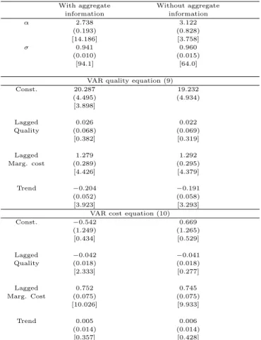
Table 2 displays all parameter estimates. The demand parameter estimates are
sensitive to the inclusion of the aggregate moment.15 There is a sizeable precision gain (highert-values) for the demand parameters. Thet-values forσgo from 64.0 to 94.1 once the aggregate information is brought to estimation. In turn,αshows an even larger precision gain, going from 3.75 to 14.18. The same is not true for the VAR estimates, which do not show considerable changes (t-values are slightly higher). This should not come as a surprise as the new moment incorporated into the model bears more directly on the demand parameters and only obliquely on VAR parameters.
Table 2 Parameter estimates
With aggregate Without aggregate
information information
α 2.738 3.122
(0.193) (0.828)
[14.186] [3.758]
σ 0.941 0.960
(0.010) (0.015)
[94.1] [64.0]
VAR quality equation (9)
Const. 20.287 19.232
(4.495) (4.934)
[3.898]
Lagged 0.026 0.022
Quality (0.068) (0.069)
[0.382] [0.319]
Lagged 1.279 1.292
Marg. cost (0.289) (0.295)
[4.426] [4.379]
Trend −0.204 −0.191
(0.052) (0.058)
[3.923] [3.293]
VAR cost equation (10)
Const. −0.542 0.669
(1.249) (1.265)
[0.434] [0.529]
Lagged −0.042 −0.041
Quality (0.018) (0.018)
[2.333] [0.277]
Lagged 0.752 0.745
Marg. Cost (0.075) (0.075)
[10.026] [9.933]
Trend 0.005 0.006
(0.014) (0.014)
[0.357] [0.428]
∗Standard deviations are in parentheses andt-values in square brackets.
6. Final Remarks
Using data from the Colombian beer industry from 1977 to 1990, I demonstrate how to extend the KLT framework by including the extra information provided by commonly available data on aggregate physical output. The idea behind the estimation procedure is to ask the structural model, parameterized by consumers’ preferences, to reproduce observed data on aggregate physical quantities. The model is then estimated through Bayesian Markov Chain Monte Carlo Methods. The results show a precision gain in the parameter estimates once the additional information is included. This precision gain, measured by thet-values, is sizeable for the demand parameters α and σ. In turn, the VAR parameters show little sensitivity to the inclusion of the aggregate variable. Although the closed form of the nested logit demand systems has some computational advantages, it comes at the cost of strong restrictions on own and cross-price effects (see Nevo (2000)). In this way, an interesting extension to this paper would consist in introducing consumer heterogeneity in a more sophisticated fashion along the same lines as BLP.
References
Ackerberg, D. & Rysman, M. (2002). Unobserved product differentiation in dis-crete choice models: Estimating price elasticities and welfare effects. NBER Working Paper 8798.
Anderson, S., De Palma, A., & Thisse, J.-F. (1992). Discrete Choice Theory of Product Differentiation. MIT Press, Cambridge, Massachusetts.
Aw, B.-Y., Chen, S., & Roberts, M. (2001). Firm-level evidence on productivity differentials and turnover in Taiwanese manufacturing.Journal of Development Economics, 66(1):51–86.
Bahk, B. & Gort, M. (1993). Decomposing learning by doing in new plants.Journal of Political Economy, 101(4):561–583.
Berry, S. (1994). Estimating discrete-choice models of product differentiation. Rand Journal, 25(2):242–262.
Berry, S., Levinsohn, J., & Pakes, A. (1995). Automobile prices in market equi-librium. Econometrica, 63(4):841–890.
Berry, S., Levinsohn, J., & Pakes, A. (1999). Voluntary export restraints in auto-mobiles. American Economic Review, 89(3):400–430.
Botasso, A. & Sembenelli, A. (2001). Market power, productivity and the EU single market program: Evidence from a panel of Italian firms. European Economic Review, 45:167–186.
Caplin, A. & Nalebuff, B. (1991). Aggregation and imperfect competition: On the existence of equilibrium. Econometrica, 59(1):25–59.
Cardell, S. (1997). Variance components structures for the extreme value and logistic distributions with application to models of heterogeneity. Econometric Theory, 13(2):185–213.
DeSouza, S. (2004). Describing Firm’s Behavior from Revenue and Cost Data. PhD thesis, Penn State University.
Gilks, W. R., Richardson, S., & Spiegelhalter, D. J. (1996).Markov Chain Monte Carlo in Practice. Chapman & Hall/CRC, Florida.
Goldberg, P. (1995). Product differentiation and oligopoly in international mar-kets: The case of the U. S. automobile industry. Econometrica, 63(4):891–952.
Griliches, Z. (1986). Productivity, R&D and basic research at the firm level in the 1970s. American Economic Review, 76(1):141–154.
Griliches, Z. & Regev, H. (1995). Firm productivity in Israeli industry: 1979-1988. Journal of Econometrics, 65(1):175–203.
Hausman, J., Leonard, G., & Zona, J. (1994). Competitive analysis with differen-tiated products. Annales d’Economie et de Statistique, 34:159–180.
Imbens, G. & Lancaster, T. (1994). Combining micro and macro data in microe-conometric models. Review of Economic Studies, 61(4):655–680.
Katayama, H., Lu, S., & Tybout, J. (2003). Why plant-level productivity studies are often misleading and an alternative approach to inference. NBER Working Paper 9617.
Klette, T. & Griliches, Z. (1996). The inconsistency of common scale estima-tors when output prices are unobserved and endogenous. Journal of Applied Econometrics, 11(4):343–61.
Klette, T. J. (1999). Market power, scale economies and productivity: Estimates from a panel of establishment data.Journal of Industrial Economics, 47:451–76.
Lahiri, K. & Gao, J. (2001). Bayesian analysis of Nested logit model by Markov chain Monte Carlo. Mimeo.
Liu, L. & Tybout, J. (1996). Productivity growth in Chile and Colombia: The role of entry, exit and learning. In Roberts, M. & Tybout, J., editors,Industrial Evolution in Developing Countries. Oxford University Press, Oxford and New York.
Mairesse, J. & Sassenou, M. (1991). R&D and productivity: A survey of econo-metric studies at the firm level. STI Review, pages 9–43. OECD, Paris.
Marshak, J. & Andrews, W. H. (1944). Random simultaneous equations and the theory of production. Econometrica, 12:143–205.
McFadden, D. (1981). Econometric models of probabilistic choice. In Manski, C. & McFadden, D., editors,Structural Analysis of Discrete Data. MIT Press, Cambridge.
Melitz, M. J. (2000). Estimating firm-level productivity in differentiated product industries. Mimeo, Harvard University.
Nevo, A. (2000). A practitioner’s guide to estimation of random-coefficients logit models of demand. Journal of Economics & Management Strategy, 9(4):513– 548.
Nevo, A. (2001). Measuring market power in the ready-to-eat cereal industry. Econometrica, 69(2):307–342.
Ocampo, J. A. & Villar, L. (1995). Colombian manufactured exports 1967-91. In Helleiner, G., editor, Manufacturing for Export in the Developing World: Problems and Possibilities. Routledge, New York, N. Y.
Pakes, A. & McGuire, P. (1994). Computing Markov-perfect Nash equilibria: Numerical implications of a dynamic differentiated product model. Journal of Economics, 25(4):555–589.
Panzar, J. & Rosse, J. (1987). Testing for ‘monopoly’ equilibrium. Journal of Industrial Economics, 35(4):443–456.
Pavcnik, N. (2002). Trade liberalization, exit and productivity improvements: Evidence from Chilean plants. Review of Economic Studies, 69(1):245–276.
Petrin, A. (2002). Quantifying the benefits of new products: The case of the minivan. Journal of Political Economy, 110(4):705–729.
Roberts, M. (1996). Colombia, 1977-85: Producer turnover, margins and trade ex-posure. In Roberts, M. & Tybout, J., editors,Industrial Evolution in Developing Countries. Oxford University Press, Oxford and New York.
Slade, M. (2004). Market power and joint dominance in U. K. brewing. Journal of Industrial Economics, 52:133–163.
Trajtenberg, M. (1990). Economic Analysis of Product Innovation: The Case of CT Scanners. Harvard University Press, Cambrige, MA.
Appendix A
Colombian Data Set
This appendix shows how Roberts (1996) constructed his data set from the survey collected by DANE.
Plant-specific identification numbers are not available on the original Colombia data set. Then, plants are matched across years by using reported values for in-ventories and capital stock and by comparing them in successive years. Inin-ventories and capital stock are unlikely to change considerably in successive years. For this reason, they were selected as matching criteria.
The original data set has information on: SIC code (at the four digit level), the year in which the plant was established, the section of the country in which the plant is located (not available in 1977 – 79) and metropolitan area in which the plant is located. Values of inventories and capital stocks are broken down into their component parts as follows:
Total inventories = finished goods + raw materials + goods in progress Total capital stock = buildings and structures + machinery and equipment
+ land + transportation equipment + office equipment
The matching algorithm goes as follows. First, observations are pre-matched on: SIC, year of establishment, section of the country and metropolitan area. Then, values for inventories and capital stocks are compared in the following order: finished goods inventories, raw materials, total inventories, buildings and struc-tures, machinery and equipment, land, transportation equipment, office equipment and total capital stock.
Appendix B
Uncovering Relevant Quantities from Revenue and Cost Data with Mul-tiplant Ownership
This appendix shows how to uncover relevant plant-level quantities from rev-enue and cost data conditional on the parameters of the model. Equation (6) in the text can be rewritten as
1 +
X
r∈Ff
(pr−mcr)
∂sr
∂pj
.
sj
= 0 (B.1)
Further, it is easy to show that the following equalities hold for the cross and own price derivatives
∂sr
∂pj
.
sj=−
α 1−σ
sr
sj
[−(1−σ)sj−σsw]
∂sj
∂pj
.
sj =−
α
1−σ[1−(1−σ)sj−σsw]
Note also thatsr/sj =qr/qj, Rj =pj.qj, T Cj =mcjqj, andsj =qj/(Q+Q0) whereRj, T Cj, Q and Q0 are revenue, total variable cost, total output produced by domestic firms and total imported quantity, respectively. Hence, substituting these equations into the pricing rule (B.1) and solving for quantity of plant j belonging to firmf (j∈Ff ), one obtains
qj=
1−σ α(Rj−T Cj)
+
(1−σ)
Q+Q0 + σ
Q
X
r∈Ff
(Rr−T Cr)
(Rj−T Cj)
−1 (B.2)
Aggregating over theqj’s results in
Q = X
f=1,2,...,N F
,X
j∈Ff
1−σ α(Rj−T Cj)
+
(1−σ)
Q+Q0 + σ
Q
X
r∈Ff
(Rr−T Cr)
(Rj−T Cj)
−1
where N F is the total number of firms. This nonlinear equation can be solved numerically forQgiven (α,R,TC, Q0), whereR={Rj;j = 1, ...N F}andTC=
{T Cj;j= 1, ...N F}. Then, given the same parameters and data,qj is determined
from (A1.2), whereas pj, mcj and sj follow trivially from pj = Rj/qj, mcj =
Finally, the log-linearized version of the demand system (8) can be solved for relative qualityaj
ajt≡ξj−ξ0=α(pj−p0)−σlnsw+ lnsj−lns0
Appendix C
Gibbs Sampler16
Although one cannot make inference directly fromL(D;θ)p(θ), it is possible to sample from the full conditionals of theθcomponents. In the NLB model, the parameter vector is divided into: θ1= (ϕ, λ), θ2= (Σ), θ3= (ν), θ4= (α, σ). The parametersϕ, λ, α, σ are defined as before, Σ is the covariance matrix of the VAR error terms andν is the variance of error in the aggregate quantity equation (10). The Gibbs algorithm goes as follows.
Step 0: Draw initial values for the parameter vector
θ0= (θ10, θ20, θ03, θ04) and seti= 0
Step 1: Drawθi+1 from the conditionals below.
1.1) Drawθi+1
1 ∼π1(θ1|θi2, θ3i, θi4, D) 1.2) Drawθi+1
2 ˜π2(θ2|θ1i+1, θ
i
3, θi4, D) 1.3) Drawθ3i+1∼π3(θ3|θ
i+1 1 , θ
i+1 2 , θ4i, D) 1.4) Drawθ4i+1∼π4(θ4|θ
i+1 1 , θ
i+1 2 , θ
i+1 3 , D)
Step 2: Seti=i+ 1 and go back to step 1.
Here πk(θk |θ−k, D) =L(D;θ).pθk(θk), wherepθk(θk) is the prior of the
sub-vectorθk. Further, to describe the conditionals, define
Yjt = (ajt,mcjt)′, Zjt= (1, ajt, mcjt, t)′, Ujt= (ǫajt, ǫ c
jt)′, and B′
=
b01ϕ ϕcβ
b02λ λcφ
In addition, let
Y = [Y12....Y1T...YN2...YN T′
Z= [Z12....Z1T...ZN2...ZN T′
U = [U12....U1T...UN2...UN T′
The VAR system can then be written as Y=XB+U. Given θ4, Y and Z are given and 1.1) to 1.3) have known probability distributions. On the other hand, π4(θ4|θ1, θ2, θ3, D) does not have a closed form solution, which requires the use of a Metropolis-Hastings (M-H) algorithm.
More specifically, definingKas one plus the number of variables appearing on the RHS of the VAR and assuming that the prior ofθ1isN(02k,100×I2k), one can
show thatπ1(θ1|θ2, θ3, θ4, D) is also a normal with meanun= [(Z′⊗Σ)V ec(Y′)]
and varianceVn=
((Z′Z)⊗Σ−1) + (1/100)I 2k
−1
.
For 1.2 it is assumed that Σ has Inverse Wishart prior with parameters 6 and 100xI2. Then π2(θ2 |θ1, θ3, θ4, D) has a distributionInvW ish(mn, G−n1), where
mn= 6+ number of observations,17 and
G−n1= (100×I2) + (Y −ZB)′(Y −ZB)
Similarly,νhas the prior distribution defined as the scalar version of the inverse Wishart (InvWish(6,100)). Hence, the conditionalπ3(θ3 |θ1, θ2, θ4, D) is also an
InvW ish(mn, G−n1), mn = 6 + (np−1), andG−n1= 100 +w′w, wherewis a vector
that collects all thewt’s.
The prior for α is uniform with support [0,10], while σ has the same prior, but its support is a little narrower [0,1]. Since one cannot identify the shape of π4(θ4 | θ1, θ2, θ3, D), θ4 has to be sampled using a random walk Metropolis-Hastings acceptance criterion with a normal proposal density. The probability
of acceptance of θ4′ is min
1,π4(θ
′
4|θ
i+1 1 ,θ
i+1 2 ,θ
i+1 3 ,D)
π4(θi4|θ
i+1 1 ,θ
i+1 2 ,θ
i+1 3 ,D)
, where θ′4 is drawn from a
normal density with meanθi
4 and variance Λ. In principle, any Λ can be used in the algorithm, however, for a well behaved convergence to the invariant probability distribution, it is recommended to calibrate this variance such that it is not too “big” (all the proposed θ′4 will be accepted, but the chain will move slowly) nor too “small” (nearly all proposed moves will be rejected and the chain may not move for several iterations).
Once convergence of the Markov chain has been attained (suppose at the Lth
simulation), it suffices to sample from the invariant distribution using the drawsθi,
wherei > L. To obtain the statistics reported in Table 1, I run 20,000 iterations of the Markov chain and setLto be 2,000. Figures 1 and 2 show the graphs of the MCMC simulations for the demand parameters for the nested logit model with the aggregate quantity. Clearly, after 2,000 iterations the Markov chain moves within a certain range and inference can be made from then on.
0 1 2 3 4 5 6 7
1
729
1457 2185 2913 3641 4369 5097 5825 6553 7281 8009 8737 9465
10193 10921 11649 12377 13105 13833 14561 15289 16017 16745 17473 18201 18929 19657
Figure 1 MCMC simulation forα
0,5 0,55 0,6 0,65 0,7 0,75 0,8 0,85 0,9 0,95 1
1 1338 2675 4012 5349 6686 8023 9360 10697 12034 13371 14708 16045 17382 18719