Estud. Econ. vol.37 número4

SERGIO AQUINO DESOUZAZZ ¸

RESUMO

Este artigo demonstra como construir um índice de preços ajustados pela qualidade sem a observação direta de dados ao nível de produto (preços, quantidades e características). A técnica aplicada no artigo permite medir a inflação dos preços com base na variação intertemporal de bem-estar através do uso de dados de receita e despesa comumente disponíveis (pelo menos para o setor industrial) ao nível de empresas. No entanto, tal técnica exige a imposição de hipóteses sobre a evolução da qualidade do bem externo assim como a estrutura da demanda e da oferta. Com dados sobre a indústria colombiana de cerveja e combi-nando metodologias originalmente desenvolvidas por Katayama, Lu e Tybout (2003), DeSouza (2006a) e Trajtenberg (1990) estimam-se os parâmetros da demanda e constroem-se índices de preços para o período de 1977 a 1990 a partir da mensuração do bem-estar dos consumidores.

PALAV

P

P RAS-CHAVE

índice de preços, inovação, modelos de escolha-discreta

ABSTRACT

This paper shows how to construct quality adjusted price indices without direct observation of product-level data (prices, quantities and characteristics). The technique used here allows for a welfare based measurement of price change using commonly available (at least for the manufacturing sector) plant–level data on revenue and cost. However, one has to be explicit about the evolution of the outside good quality and the structure of demand and supply. Using data on the Colombian beer industry and combining the methodologies originally proposed by Katayama, Lu and Tybout (2003), DeSouza (2006a) and Trajten-berg (1990) I am able to uncover the demand parameters and build welfare-based price indices for the 1977-1990 period.

KEY WORDS

price index, innovation, discrete-choice demand models

JEL CLASSIFICATION

E31,L66,O33

Ø I would like to thank James Tybout, Mark Roberts and two anonymous referees for their useful comments. I am also thankful to CAPES and FUNCAP for providing financial support to this work.

¸ _{Professor Adjunto do Curso de pós-graduação em Economia - CAEN/UFC e do Departamento de Teoria}

Econômi-ca da Universidade Federal do Ceará - Av. da Universidade, 2700, 2º andar - Fortaleza - Ceará. Tel/Fax: 55-85-4009-7751. E-mail: [email protected]

I. INTRODUCTION

Most statistical institutions report price indexes calculated from a weighted average of prices. A better way to measure price changes, known as the hedonic price approach, consists of regressing observed prices (in logs) on product characteristics, to control for quality variation, and time dummies. These dummies are interpreted as the incre-ase in price net of quality improvements. The hedonic strategy, however, has its own limitations, as it places great demands on the data set. The statistical agency has to define what characteristics are relevant in determining prices. The agency also has to observe (or collect) prices and characteristics of many products offered in the market. With the development of discrete choice models another technique has been proposed (Trajtenberg, 1990). The basic idea consists of uncovering the true price change from the variation in consumer surplus which is calculated after estimating the parameters

of a discrete-choice demand system. The strategy goes as follows: i. setup a theoretical

model of consumer choice1_{, ii. match the model’s prediction about economic variables}

(e.g., prices and quantities) to their empirical counterparts to obtain the relevant

pa-rameters, iii. from these parameters, calculate the price variation that would have had

the same welfare effect as the innovations that actually took place.2

Steps i and ii can be undertaken using traditional discrete-choice models found in

the Industrial Organization literature (e.g. Berry, 1994). The original contribution

of Trajtenberg comes from step iii. Using the structural approach outlined in the

previous steps, he shows how to construct quality-adjusted price indices for a specific

product.3 Berry’s approach to estimate demand, and possibly supply, parameters places

even greater demands on the data as not only prices but also quantities have to be observed at the product-level.

Detailed data set, as required by the hedonic and berry’s approach, may be difficult or costly to obtain in many instances. Confidentiality issues and/or strategic purposes may induce some firms not to release the relevant data. On the other hand, official statistical agencies are usually more successful in the task of gathering information for plant-level surveys of the manufacturing sector. One of the reasons may rely on the fact that, in many cases, firms are asked to report only sales revenue and input

1 Sometimes, modeling producers’ choices is useful to undertake step ii.

2 A notorious example of such approach can be found in Nevo (2003). He uses discrete-choice de-mand parameters, estimated from cross section of product level data, to compute welfare-based price indices.

expenditures, rather than (more revealing) strategic information on prices and quan-tities. Such surveys are commonly available for many countries and cover most in-dustries in the manufacturing sector, providing an easily accessible source for applied researchers.

The data set used here falls within the class of data sets discussed in the last paragra-ph. It reports only plant-level revenue and total cost instead of price and quantities,

hampering initial attempts to undertake steps i and ii according to the standard

approach found in Berry’s work. To overcome this restriction, Katayama, Lu and Tybout (2003), KLT henceforth, builds on berry’s work and devise an econometric methodology to uncover the demand parameters set as well as marginal costs, quality, prices and quantities from plant-level data that report only revenue and cost data. A similar methodology is developed by DeSouza (2006a). However, instead of estima-tion through econometric techniques, the methodology found in DeSouza (2006a) takes advantage of the extra information provided by aggregate data to calibrate the relevant parameters and variables. Although it may be difficult to obtain detailed data on quantities at the plant level, the same is not true for aggregate variables. For ins-tance, in the beverage sector, the amount of beer, in liters, consumed in a given year is widely available for many countries. Aggregate quantities also carry information on demand parameters and therefore may help in determining their magnitudes.

This paper shows how to construct quality-adjusted price indices when only revenue and cost data are observed. Indeed, by applying the methodologies mentioned above to the Colombian beer market, it is possible to uncover the demand parameters and construct welfare-based price indices. This paper is organized as follows. The second section introduces the demand discrete-choice model, the consumer surplus function and a model of firms’ supply. This section also includes the description of the empi-rical strategies mentioned above. The ensuing section comments on the beer market idiosyncrasies and presents the demand parameters estimates. The fourth section discusses the methodology to uncover the quality adjusted price indices, introduces consumer surplus identification issues, and presents the index numbers. Finally, the last section adds a few remarks and suggestions for future work.

II. THEORETICAL MODEL AND EMPIRICAL STRATEGIES

Demand

Consumers rank products according to their characteristics and prices. There are

N+1 choices in the market, N inside goods (domestic varieties) and one outside good

(imported variety). Consumer i chooses a good j, given price pj, (unobserved)

charac-teristics [j, and unobserved idiosyncratic preferences. Products are grouped into two

nests, indexed by g, which takes the values of 0 or 1. The first nest (g=0) contains

only the outside good (imported variety in this application) whereas the second (g=1)

contains the N inside goods (domestic varieties).

Then, for product j belonging to nest g define utility of consumer i as

(1

)

ij j ig ij

u

G 9 V H

for j=0,1,..,N (1)

where, Gj is the mean utility, which is given by the sum of a scalar summarizing

unob-served product characteristics4 (

[

j) and income disutility (

D

p

j), i.e.,

G [ D

j j

p

j.

The first random term (

9

ig) on the right hand side (RHS) of the equation above is a

common shock to all products in nest g and its distribution depends on the parameter

V (0d V 1). As V approaches zero the within correlation of utilities within each

nest decreases, and as V approaches one the within correlation increases. The second

random term

H

ij is identically and independently distributed extreme value. McFadden

(1981) shows that we can integrate out

9 V H

_ig

(1

)

_ij to obtain a closed form

solu-tion for the within aggregate market shares (swj) for an inside good as follows

0

0 1

exp[(

) / (1

)]

exp[(

) / (1

)]

j

j N

k k

sw

G G

V

G G

V

¦

, j=1,2,…,N

Here, G is the outside good mean utility (

G D [

0

p

0 0). The share of all domestic

brands is given by

s

_d

D

/(

D

1

)

, where

1

0 1

exp[(

) / (1

)]

N

k k

D

V

­

_{G G}

_V

½

®

¾

¯

¦

¿

. Thus

the market share for a domestic variety sjis given by

0

0 1

exp[( ) / (1 )] .

1 exp[( ) / (1 )]

j j N k k D s D § ·

¨ _{G G V} ¸ _{ª º}

¨ ¸ _{« »}

¨ _{G G V} ¸ ¬ ¼

¨ ¸

©

¦

¹

(2)

which is simply the product of swj times sd.

Further, taking the log-difference between sj and s0 the demand system takes the

sim-ple log-linear functional form

0 0 0

ln

s

_j

ln

s

D

.(

p

_j

p

)

V

ln

s

_wj

[ [

_j (3)

Supply

Each firm f produces a subset Ff of the goods sold in this market and set prices in a

Bertrand game to maximize the sum of profits

3

f , which is given by

(

).

.

f

f j j j

j F

p

mc

M s



3

¦

₍₄₎

where Mis the total market size and mcj is the marginal cost of producing brand j.

Then, it can be shown that the price pjof any product j produced by firm f must

sa-tisfy the following equation

(

)

0

f

r

j r r

r F j

s

s

p

mc

p



w

w

¦

(5)

Note that (5) is flexible enough to accommodate different market structures. The first is the single firm product, in which the firm can only control the price of its unique brand. The second is the multi-product firm, in which the firm internalizes the pri-ce decision of all of its brands. The third is a monopoly firm who owns all brands available in the market. In this case, the Bertrand game degenerates to a single-agent decision problem.

Empirical Methods

If prices and quantities were available all the parameters of the model could be esti-mated through GMM using demand and supply side moments. Indeed, notice that, under some rearrangements, (3) provides a closed form for the demand system that

can be solved, up to the model parameters, for the unobservable term

[ [

j 0. The

unobservable (

[ [

j 0) can be combined with appropriate instruments (product

Fortunately, KLT, building on berry’s work, show that commonly available infor-mation on revenue and total costs (not prices and quantities) can be used to uncover the relevant variables. Their algorithm- henceforth referred to as the transformation algorithm- goes as follows.

Note that firm j’s revenue (Rj) and variable cost5( TCj) can be written as Rj=pj.qj,

TCj=mcj.qj, where qj represents firm j’s output. Thus, we can write the market share

for firm j as sj=qj/(Q+Q0), where Q and Q0 represent the total output produced by

domestic firms and total imported quantity, respectively. Then, these three identi-ties (revenue, cost and market share) together with the F.O.C (5) can be solved for

quantity as a function of data (R,TC,Q0) and the demand parameters (D,V), where R

collects the revenue of all plants in the sample and TC _{collects the costs of all plants}

in the sample.

Similarly, we can retrieve mcj=mcj(D,V,R,TC, Q ,Q0), pj= pj(D,V,R,TC, Q ,Q0) and qj=

qj(D,V,R,TC, Q ,Q0). Thus, from _j

( , ,

N

q

D V

¦

R,TC,

Q

,

Q

₀

)

Q

, we are able to solve

for Q=Q(D,V,R,TC,Q0). Then, conditional on the models’ parameters, we can retrieve

prices, quantities and market shares. Thus, relative quality, defined as

a

jt

[ [

jt 0t,

can be determined from the demand system (3). To summarize, given (D,V,R _,TC,Q0),

the KLT transformation algorithm6 shows how to obtain firm level prices, marginal

costs, relative quality and quantities as well as aggregate output (Q).

With the transformation algorithm in hand it is possible to determine the model parameters using two different (but closely related) approaches. The first one also

comes from KLT. They assume a VAR process for the co-movements of ajt and mcjt

and prior distributions on the parameters, updated by data according to the Bayesian rule to obtain the posterior distributions, from which inference is made. The second method, developed by DeSouza (2006a), relies heavily on the transformation algori-thm laid out above, but does not require the imposition of a VAR. Shortly, it consists of matching the aggregate output implied by the structural model to its observed

counterpart in order to calibrate the relevant parameter set.7 Appendix B discusses

these two methods in more depth.

5 TCj=mcj.qj as long as marginal costs are flat.

6 For more details, see Appendix A.

III. DATA AND PARAMETER ESTIMATES

The data set consists of an unbalanced panel of plants in the beer industry, with more than 10 employees, covering the period from 1977 to 1990. Originally, the data were

gathered by the Colombia’s Departamento Nacional de Estadistica (DANE) and have

been cleaned as described in Roberts (1996). The revenue series are constructed as the total sale revenue divided by a general wholesale price deflator. The total variable costs are defined as the sum of payments to labor, intermediate input purchases and energy purchases. Since some of the cost is incurred in the export activity we have to scale it by the ratio of total domestic sales to total sales and deflate the result by the same wholesale price deflator mentioned before. Note that prices and quantities are not directly observed. Therefore, the methodologies described in the second section have to be used.

From an additional source (the United Nations database) I obtain the quantity of beer (in hectoliters) produced in the country for the same sample period. Ideally, we would want to have data on the quantity of beer consumed in the country. However, the data in hand is not so restrictive since there is very little export activity in this sector.

I also use auxiliary data to uncover the price of the imported good (p0t) 8 as well as

its imported quantity in hectoliters (q0t). In a separate publication DANE also reports

the net weight (in kilos) and the monetary value of imports (in pesos). Assuming that beer has the same density as water (1kg per liter), it is easy to transform the net

weight in kilos to volume of imported beer in hectoliters (q0t). Then, p0t follows from

the ratio of the peso value of imports to q0t.

While it is common for data sets to report plant-level revenue and cost data, they do not usually contain information on plant ownership. This is important for estimation since each ownership arrangement implies a different supply function and therefore,

given (D,V,Rjt ,TCjt,Q0t), different values for the unobserved variables (price,

quanti-ties, marginal cost and qualities). In the Colombian beer sector, however, ownership is not an issue since one Company (Bavaria S.A) controlled the non-imported beer market during the sample period studied here.

Indeed, after an aggressive horizontal merger strategy, Bavaria became the dominant

firm in the beer production by acquiring its rivals (Cerveceria Aguila, Cerveceria Union

andCerveceria Andina and other smaller producers) in the beer business by the early

seventies. Its dominance went unchallenged until 1995 when Cerveceria Leona entered

the beer market as retaliation for the Bavaria entry in the soft drinks business, which

was controlled by Leona’s parent company. Since the data sample period ranges from 1977 to 1990 all the estimations presented below assume that a single firm owns all plants.

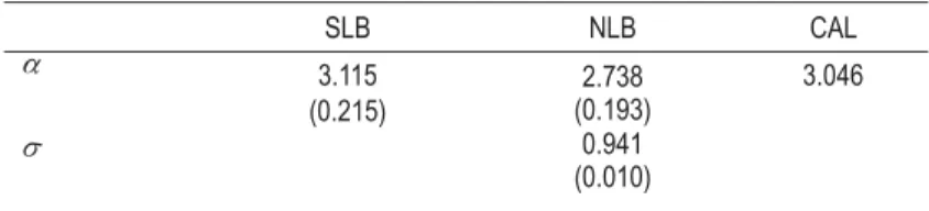
The parameters estimates are displayed below in table 1. Three different models are

con-sidered: the Nested Logit model (0 V 1) and the Simple Logit model (V 0), both

based on Bayesian techniques (NLB and SLB henceforth) and the Simple Logit mo-del, implemented according to the calibration approach found in DeSouza (2006a)-

this method will be referred to as CAL from now on).9

TABLE 1 – PAR AMETERS ESTIM ATES*

SLB NLB CAL

D _3.115

(0.215)

2.738 (0.193)

3.046

V 0.941

(0.010)

* Standard deviation in parentheses.

When compared to the simple logit models, the NLB yields lower estimates for price

disutility D and high estimates for the within value V, which means that the set of

the inside goods (domestic goods) is highly differentiated from the outside good

(imported variety). Notice also that although D is allowed to vary over time in the

CAL setting, its mean (3.04) is about the same magnitude as the price coefficients estimates for both Bayesian models.

IV. QUALITY ADJUSTED PRICE INDEX

The most popular method to obtain quality-adjusted price changes is given by the hedonic equation. Price is the dependent variable and product characteristics and time dummies are the RHS variables. The price change that is not explained by improvements in product characteristics is the true price variation. One problem with this approach consists of choosing the set of characteristics that are relevant to determine prices. There is always a high degree of discretion in setting up the hedo-nic regression. Different characteristics bundles may affect the index calculation. For instance, if gas mileage is omitted in the hedonic price regression for new cars, and a given car improves its fuel efficiency, the index would overstate the true change in prices, for this variable would be captured by the regression error term and not by

the regressors. In some data sets, like the one used in this paper, not even product characteristics are observed.

Another methodology was devised by Trajtenberg (1990). The basic idea consists of uncovering the true price change from the variation in consumer surplus which is calculated from the parameters of a discrete-choice demand system. Below, I lay out his methodology in more detail.

Trajtenberg Method

Once the demand parameters of the discrete choice model are estimated, the consu-mer surplus for the Nested Logit model can be calculated from the following equation (McFadden ,1981)

1

0

1

( ,

)

ln

exp[(

) / (1

)]

t

N

t t t kt kt

k

CS P

p

V

§

·

[

_¨

[ D

V

_¸

D ©

¦

¹

G

G

(6)

where

P

G

_t denotes the vector that comprises all prices pjt at time t and

[

t

G

the vector

that contains all the

[

jt’s at time t. The consumer surplus for the simple logit model

is calculated by simply setting V =0. The intertemporal variation in consumer surplus

is then given by

'

CS

t

CS P

t

( ;

t

[

t

)

CS

t1

(

P

t1

;

[

t1

)

G

G

G

G

.

McFadden (1981) also shows that 'CSt can be written as a difference between two

expenditure functions (

'

CS

t

e P

(

t1

,

[

t1

)

e P

(

t

,

[

t

)

G

G

G

G

, where e(.) is the expenditure

function ). Then, the price index obtains after solving for Ut from the following

equality10

1 1 1

(

,

)

((1

)

,

)

t t t t t t

CS

e P

e

P

'

G

[

G

U

G

[

G

(7)

The variable Ut, known as the welfare equivalent price reduction, measures the

hy-pothetical average price reduction that would have had the same welfare effect as the innovations (or quality improvements) that actually took place. In other words, consumers would have been equally well off if they had been offered the old set of

products at prices lower by a factor of Ut. This factor follows the same qualitative

movements as 'CSt. For example, suppose nominal prices remain the same, then the

larger is the increase in quality the larger is the price reduction Ut. Consumers would

demand a lower price to compensate for a worse set of products. For obvious reasons consumer surplus would also increase with higher quality.

Solving (7) involves a highly nonlinear equation. A simple solution was derived by

Trajtenberg (1990). After assuming mild restrictions11 _{on the average price change}

he shows that

1 t t t

CS

p

'

U

(8)

where

p

tis the unweighted average price across firms at period t. The price index (It)

is then constructed by the simple formula

1

(1

)

t

t t

I

I

U

with I0=100.

The unobservable [j has an interesting interpretation that is particularly important

in the context of price indices. It can be viewed as the unobserved quality of product

j. Thus, unlike the hedonic price index, the welfare based index captures changes in

omitted attributes. Also, since consumer surplus is a function of prices and attributes

of all the goods available to consumers at a certain period t, the temporal variation

of surplus provides a natural way to control for the entry of new products. On the other hand, the major limitation for the practical use of this method by statistical agencies hinges on the data requirement. It demands data on prices for virtually all firms active in the market, otherwise demand and supply could not be estimated properly. Obviously, gathering such a comprehensive data set is very costly making it difficult to consider such technique as a practical substitute for the hedonic price index. Fortunately, as show in the section II, KLT and DeSouza (2006a) offer me-thods to uncover the demand parameter set and pin down price and (relative) quality using commonly available firm level data on revenue and cost for firms in the manu-facturing sector. But, before, constructing the price index it is important to discuss identification issues regarding the consumer surplus variation.

Identification Issues

The demand system only permits the identification of the relative movements in

qua-lity of the inside goods with respect to the outside good (recall that

a

j

{ [ [

j 0).

Then, unless we postulate an assumption on the evolution of the outside good, it is

11 The price of each brand can always be written as pit pt 'pit, where pt is the unweighted average across

brands. Assume now that the intertemporal price variation takes the form pit U(1 t)pt1 'pit1, i.e, the

distribution moves leftward by a factor (1-Ut) but the variance remains the same. Then, (8) follows easily

not possible to identify the intertemporal variation in consumer surplus (¨6t). To

cla-rify this point note that, from (6) ,¨&6tcan be rewritten as

1

0

0

0 0

1 1 0 1

0

( )

exp

1 1

(1 ) ln

( )

exp

1

t

t

N

kt kt t

t t t N

kt kt t

a p p

CS p

a p p

ª § ­ D ½ ·º

® ¾

« ¨ _{¯ V ¿} ¸»

« ¨ ¸»

' '[ D' V

« »

D ¨ ­ D ½¸

® ¾

« ¨_{© ¯ V ¿}¸_¹»

¬ ¼

¦

¦

(9)

Once the demand parameters are determined from the techniques describe in section

II, all terms but

'[

0t can be identified. The lack of identification of

'[

0t has quite

different consequences for welfare variation.

For example, relative quality could go up due to different reasons. First, the inside good could become more attractive. Alternatively, the outside good attractiveness could fall instead. In the former case, welfare would increase while in the latter it would decrease. Thus, we have to be explicit about the assumptions on the evolution of the outside good. Below, I make an assumption that help to identify the absolute

quality movements.12

Assumption: the quality of the outside good does not change over time, i.e,

'[

_0t=0

for all t.

This assumes away the identification problem by imposing that all the variation in relative quality is due to the variation in product appeal of the inside goods. The ex-tent to which this assumption is appropriate will depend on the characteristics of each market. In some instances, especially in developing countries, the imported variety exhibits much more innovation than its domestic counterpart.

Calculating the Quality-adjusted price index

At this point, it is useful to summarize in a few steps how the methodologies presen-ted in this paper can be combined to determine the quality-adjuspresen-ted price index.

1- Calculate de demand parameters using either the econometric (Bayesian) method or the calibration (CAL) approach. Note: The CAL model is simple to estimate and is perhaps better suited for agencies and students who are reluctant to incur the relatively high computational cost of the Bayesian Monte Carlo technique.

2- Given the demand parameters, recover the pj’sandaj’s from the transformation

al-gorithm and determine the welfare equivalent price reduction Ut. It follows, from

the assumption defined above and equations (8) and (9), that Ut can be computed

as

0

0 0

1 1 1 0 1

0

( )

exp

1 1

(1 ) ln

( ) exp 1 t t N

kt kt t

t t N

t kt kt t

a p p

p

p a p p

ª § ­ D ½ ·º

® ¾

« ¨ _{¯ V ¿} ¸»

« ¨ ¸»

U D' V

« »

D ¨ ­ D ½¸

® ¾

« ¨_{© ¯ V ¿}¸_¹»

¬ ¼

¦

¦

(10)

Notice that for the simple logit model (V=0)

3- Compute the index from the simple formula

1

(1

)

t t t

I

I

U

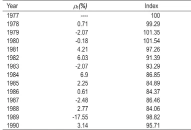
with I0=100.

The consumer surplus variation implies (according to the SLB model)13 an equivalent

price reduction of only 4.29 % (see Table 2) throughout the sample period. It means

that at the end of 1990 consumers demand a reduction in prices of 4.29%14 to go

back to 1977 set of products.

TABLE 2 – WELFARE EQUIVALENT PRICE REDUCTION AND THE PRICE INDEX(SLB MODEL)

Year Ut(%) Index

1977 ---- 100

1978 0.71 99.29

1979 -2.07 101.35

1980 -0.18 101.54

1981 4.21 97.26

1982 6.03 91.39

1983 -2.07 93.29

1984 6.9 86.85

1985 2.25 84.89

1986 0.61 84.37

1987 -2.48 86.46

1988 2.77 84.06

1989 -17.55 98.82

1990 3.14 95.71

Using the NLB estimates to construct the price indices (Table 3) I find results of the same order of magnitude for the welfare equivalent price reduction throughout the sample period (2.37%). In turn, Table 4 shows that the CAL model diverges from both NLB and SLB. In this case, consumer demand a price increase to return to the 1977 settings, meaning that welfare must have decreased on the 1977-1990 period.

The lack of robustness may be due to the fact that, unlike the Bayesian methods, Dt

can be determined for each time period and therefore welfare variation also accounts for intertemporal differences in this parameter.

TABLE 3 – WELFARE EQUIVALENT PRICE REDUCTION THE PRICE INDEX (NLB MODEL)

Year ȡt(%) Index

1977 --- 100.00

1978 0.42 99.57

1979 -1.72 101.29

1980 -0.2 101.50

1981 3.48 97.97

1982 5.79 92.29

1983 -1.9 94.04

1984 5.24 89.11

1985 1.34 87.91

1986 1.26 86.80

1987 -2.15 88.67

1988 1.23 87.57

1989 -14.46 100.24

TABLE 4 –WELFARE EQUIVALENT PRICE REDUCTION THE PRICE INDEX (CAL MODEL)

Year ȡt(%) Index

1977 ---- 100

1978 4.43 95.56

1979 0.06 95.50

1980 -1.11 96.56

1981 -1.49 98.00

1982 -0.6 98.60

1983 -4.75 103.29

1984 1.64 101.59

1985 0.83 100.74

1986 -2.17 102.93

1987 -6.53 109.66

1988 13.78 94.54

1989 -13.15 106.98

1990 -0.63 107.65

Whether the assumption of time invariant quality of the outside good is suitable is largely an empirical matter and depends on the idiosyncrasies of each market. This assumption has less appeal for markets where the imported good is much more likely to exhibit significant temporal variation. For example, in most developing countries, imported vehicles exhibit much more quality improvements than the ones produced domestically.

VI. FINAL REMARKS

This work could be reproduced to build price indices for specific manufactured products in many other countries. Data sets that share the same limitations as the Colombian survey, i.e. that contain information only on revenues and costs not pri-ces or quantities, are available for Chile, Mexico and Turkey, for example. In Brazil,

the main information source is provided by the Pesquisa Industrial Anual, a survey of

Brazilian firms and plants conducted annually by the Brazilian census bureau IBGE

(see Muendler, 2003, for a detailed description of the data set).

APPENDIX A – (THE TRANSFORMATION ALGORITHM). UNCOVERING REL-EVANT QUANTITIES FROM REVENUE AND COST DATA WITH MULTI-PLANT OWNERSHIP

This appendix paraphrases DeSouza (2006b) and is included here for the sake of clarity. It shows how to uncover relevant plant-level quantities from revenue and cost data up to some parameters of the model. Note that Equation (5) in the text can be rewritten as

1

(

)

0

f

r

r r j

r F j

s

p

mc

s

p



w

w

¦

(A1. 1)

Further, after some algebraic manipulations it can be shown that the following equa-lities hold for the cross and own price derivatives

[ (1

)

]

1

r r

j j w

j j

s

s

s

s

s

p

s

D

w

_V

_V

w

V

[1 (1

)

]

1

j

j j w

j

s

s

s

s

p

w

D

V

V

w

V

Note that

s s

r j

q q

r j, Rj=pj.qj, TCj=mcj.qj, and sj=qj/(Q+Q0) where Rj ,TCj, Q and

Q0 are revenue, total variable cost, total output produced by domestic firms and total

imported quantity respectively. Hence, substituting these equations into the pricing

rule and solving for quantity of plant j belonging to firm f (j Ff) we obtain

1

0

(

)

1

(1

)

.

.(

)

_f

(

)

r r j

r F

j j j j

R

TC

q

R

TC

Q Q

Q

R

TC



§

_V

§

_§

_V

_V

_·

·

·

¨

¨

_¨

¨

¸

¸

_¸

¸

¨

_D

_©

_©

_¹

_¹

¸

©

¦

¹

(A1. 2)

Aggregating over the qj’s results in

1

1,2,.. 0

(

)

1

(1

)

.

.(

)

(

)

f f

r r

f N j F j j r F j j

R

TC

Q

R

TC

Q Q

Q

R

TC

 

§

V

§

§

V

V

·

·

·

¨

¨

_¨

_¨

_¸

¸

_¸

¸

¨

_D

_©

_©

_¹

_¹

¸

©

¹

¦ ¦

¦

where N is the total number of firms. This non-linear equation can be solved

determined from (A1. 2), whereas pj , mcj , sj and sw follow trivially from

p

j

R q

j j,

j j j

mc

TC

q

, sj=qj/(Q+Q0) and swj=qj/Q respectively.

Finally, the log-linearized version of the demand system (3) can be solved for relative

quality aj

0

.(

0

)

ln

ln

ln

0

jt j j wj j

a

{ [ [ D

p

p

V

s

s

s

APPENDIX B – EMPIRICAL METHODS

Econometric Method

Dynamics is introduced into the model through the assumption that relative quality

and marginal cost follow an exogenous15 VAR process given by

01 1 1

c a

jt jt jt jt

a

b

I

a

I

mc

E H

t

(11)

02 1 1

a c

jt jt jt jt

mc

b

O

mc

O

a

M H

t

(12)

From the demand system, the price setting game and the VAR we are able to uncover

demand and supply side “errors”, represented respectively by

H

cjtand

a jt

H

. At this point

the model seems very close to Berry’s methodology where similar error terms are combined with exogenous product characteristics to form the identifying moment conditions. Here, however, these data are not available. Note that not even prices or quantities are observed; they are themselves functions of data and demand parameters to be estimated from the model. The model is therefore not identified such that tra-ditional econometric technique like GMM and ML do not apply.

To identify it more structure has to be imposed on the parameters. This is achieved by assuming a prior knowledge of the parameters distribution and using the data set and the structure imposed by the model to update this prior according to the Bayes rule

( ;

)

(

; ). ( )

p

T

D

v

L D

T

p

T

The LHS is the posterior probability updated by the data D, and the RHS is the

product of the likelihood function of the data times the prior distribution of the pa-rameters. However, only in special cases, the posterior distribution has a closed form from which we can make inference either by sampling from it or by consulting easily available tables. Fortunately, Monte Carlo techniques have been developed to deal with such problem. Shortly, it relies on ergodic theory to guarantee that a computable statistic converges to the true posterior distribution. Then, once convergence has been

attained, we can sample from this statistic and make inference.16

Calibration Strategy

Aggregate quantities also carry information on demand parameters and therefore may help to pin down the demand parameters. Assume now that the amount of beer, in hectoliters, consumed in a given year is observed.

Note that the model implies an aggregate quantity given some parameters and data. We can then ask the model to match this observed quantity according to

0

(

,

,

,

)

obs t t jt jt t

Q

D

R TC

Q

Q

(13)

All data in this equation are observed which implies that Dtcan be determined for

each time period t. Nevertheless, the equation above embodies a few assumptions on

the nature of the aggregate measure and on the consumer preferences. Note that it requires that the quantity implied by the model matches exactly its empirical counter-part and that the discrete choice model is the simple logit form instead of its nested

version (V=0). These assumptions do not come without a cost. First, the simple logit

model places very restrictive assumptions on consumer preferences such that

cross-price elasticities have somewhat undesirable properties.17 Second, it requires a very

reliable source for the total quantity since measurement error is not allowed.

16 See KLT and DeSouza (2006b) for additional details about the Bayesian methodology.

Given these drawbacks, a legitimate question may arise. Why bother making these restrictions on the model? The reason is that the Bayesian technique proved to be a little cumbersome to implement computationally and many government agencies and students are somewhat reluctant to adopt the Bayesian approach, especially one that requires Monte Carlo simulation. This technique also requires the imposition of priors on the parameters distribution, which even some leading researches are reluctant to do. Also, the calibration requires only data on a cross-section of firms in a given year while the identification of the Bayesian model demands a panel with at least three years of observation since it requires a VAR estimation.

REFERENCES

Berry, S. Estimating Discrete-Choice Models of Product Differentiation. RAND Journal of Economics, 25 (2), p. 242-262, 1994.

Berry, S.; Levinsohn, J.; Pakes, A. Automobile Prices in Market Equilibrium. Econo-metrica, 63(4), p. 841-890, 1995.

DeSouza, S. Studying Differentiated Product Industries using Plant-Level Data. Economics Bulletin, v. 12, n. 3, p.1-11, 2006a.

__________. Combining Aggregate and Plant-Level Data to estimate a Discrete-Choice Demand Model. Brazilian Review of Econometrics, v. 26, n.2, p. 213-234, 2006b.

Katayama, H.; Lu, S.; Tybout, J. Why Plant-Level Productivity Studies Are Often misleading, and an Alternative Approach to Inference. NBER Working Paper N°.9617, 2003.

Lu, S.; Tybout, J. Import-Competition and Industrial Evolution: A Computational Ex-periment. (mimeo). Penn State University, 2000.

McFadden, D. Econometric Models of Probabilistic Choice. In: Manski, C; McFad-den, D. (Eds). Structural Analysis of Discrete Data, 1981.

Muendler, M. The Database Pesquisa Industrial Anual 1986-2001: a Detective’s Report. (mimeo). UC, San Diego, 2003.

Nevo, A. New Products, Quality Changes and Welfare Measures Computed from Estimated Demand Systems. The Review of Economics and Statistics, 85(2), p.266-275, 2003.

Pakes, A.; McGuire, P. Computing Markov-Perfect Nash Equilibria: Numerical Implications of a Dynamic Differentiated Product Model. RAND Journal of Economics, 25(4), p. 555-589, 1994.

Timmins, C. Estimating spatial differences in the Brazilian cost of living with house-hold location choices. Journal of Development Economics, 80, p. 59-83, 2006.