http://dx.doi.org/10.1590/S1982-21702013000400009
USE OF CONTROL CHARTS FOR MULTI-TEMPORAL
ANALYSIS OF GEODETIC AUSCULTATION DATA FROM
DAMS
Uso de gráficos de controle para análise multitemporal de dados de auscultação geodésica de barragens
JOSÉ ALBERTO QUINTANILHA1 LINDA LEE HO2
CLÁUDIA APARECIDA SOARES MACHADO1 DENIZAR BLITZKOW1
1
Department of Transportation Engineering – PTR
2
Department of Production Engineering – PRO
Polytechnic School of the University of São Paulo (Escola Politécnica da Universidade de São Paulo) – EPUSP
[email protected]; [email protected]; [email protected]; [email protected]
ABSTRACT
Geodesic auscultation can be used to monitor the movement of dam structures by measuring the distance, at different epochs from fixed positions (pillars) to other positions (targets). It is important to identify the targets that present atypical measurements to permit managers to take corrective actions. After fitting a model using the Least Squares Method (LSM), the residuals normally display random behavior. Multivariate control charts are then applied to the residuals of the fitted model from data taken of geodesic survey campaigns conducted at different epochs. Control charts have been widely applied in other fields of research than production processes such as public health, marketing, services. The results show that it is possible for monitoring the multi-temporal stability by the multivariate control charts. The method provides complementary information than the classical univariate statistical analysis.
Keywords: Dam auscultation; Multivariate Control Charts; Multi-Temporal
RESUMO
A auscultação geodésica de barragens é uma das formas de monitorar a movimentação da obra através de medidas de distância, (em várias épocas) de posições consideradas fixas, os pilares, a outras posições, comumente chamadas de alvos. Desta forma é importante identificar os alvos que apresentam medidas muito atípicas de modo que os gestores possam tomar iniciativas corretivas. Após o ajuste de um modelo pelo Método dos Mínimos Quadrados (MMQ), é razoável esperar que os resíduos apresentem comportamento aleatório. A verificação disto é realizada através da construção de gráfico de controle multivariado aplicado aos resíduos do modelo ajustado com os dados provenientes de campanhas geodésicas, efetuadas em diferentes épocas. Os referidos gráficos têm sido largamente aplicados em outras áreas de ciência, como em assuntos de saúde pública, marketing, serviços, além de processos de produção. Os resultados mostram que é possível verificar uma estabilidade multitemporal através da aplicação de gráficos de controle multivariado, provendo informações complementares àquelas advindas das análises univariadas tradicionais.
Palavras-chave: Auscultação de Barragens; Gráficos de Controle Multivariado;
Controle de Qualidade; Monitoramento Multitemporal; Variância Generalizada; T2 de Hotelling.
1. INTRODUCTION
Geodesic auscultation of dams is a method of understanding and controlling the movement of the dam structure. Distance measurements are regularly carried out over different epochs from fixed positions – such as pillars – to other positions, which are usually called targets. These distances (or angles) should not vary significantly over time, and the variations, measure by the residuals, which do appear in these measurements, should be small (near zero) and random. It is extremely important to identify the targets that present atypical measurements because these must be explained and their causes identified and, when it is possible, eliminated.
This objective of this article is to present a proposal for monitoring multi-temporal data derived from geodesic survey campaigns by applying multivariate control charts. Although this quality tool has usually been employed to monitor production processes in industrial fields, its use has expanded to include other areas of research than production processes such as public health, marketing, services.
Multivariate control charts are built with residuals obtained from a fitted model by the Least Squares Method (LSM) at different measurement points over time (i.e., using every individual survey campaign, each conducted at a specific time – a particular time of the year in a particular year – but jointly treated).
2. LITERATURE REVIEW
2.1 Ordinary Tests
The statistical techniques commonly used in the literature refer to both the analysis of residuals and to the analysis of the stability of the estimated parameters of the fitted model.
After completed the fitness of the model, the following tests are usually applied (SEVILLA et al.1990): the Chi-Square statistic to verify the quality of the residuals (and goodness of fit); the F statistic to test the unit variance; Student’s t-test to identify for systematic errors; and Pope’s t-test to detect outliers.
These univariate tests comprise the usual statistical tests to make inferences on the single mean and variance and equality between two variances. These tests are applied to each set of results from each survey campaign. In the case of making inference on the mean, Student’s t-test is used to monitor if the expected mean value remains stable equal to a known value. Similarly, Chi-Square statistic (χ2) is used to verify the stability of the variance.
In any least squares adjustment, the first test concerns on the variance factor. This test verifies if the residuals are consistent with the precision of the measurements obtained from a long-run term. In practice, the test infers if the residuals are those expected, based on the precision of measurements as well as the reliability of the mathematical model.
In a model fitted by LSM (GEMAEL, 1994), the sample variance – usually represented by
S
02 based on the variance of the residuals is the statistics used to monitor if the variance remains stable equal to a reference variance which is initially assumed to be equal to one (called as a priori variance). Rejection of this null hypothesis may be an indicator that gross errors are present (“blunder” values) or that the fitted model may be equivocal. In this case, the residuals do not follow a normal distribution and the observed values that seem to be inconsistent with the measured values.Once performed the variance factor test, the residuals should be individually analyzed to verify whether they constitute gross errors. Although this procedure is only absolutely necessary when the global test (
S
02) is rejected, it is always applied as the global test acceptance does not guarantee the presence of gross errors. If the null hypothesis of the global test is not rejected, the sample is considered representative of the population; otherwise, an approximation and the standardized residuals are used.The stability of the parameters is verified by comparing the results measured in two epochs using the so-called Global Congruency Test (GCT), as described in Niemeier (1981), Caspary et al. (1990), Denli and Deniz (2003), and Marotta et al. (2013). This test aims to determine the temporal stability of points from a network of deformations and/or structures control; the test defines which points remain stable and can be used in the determination of targets, which are the objects of the deformation analysis.
According to Giles (2000), the Anderson-Darling test is widely used and displays good properties. It is a nonparametric test to test the null hypothesis that a sample of size n taken from a population (with an unknown mean and variance) follows a specific distribution function. In the current case, it is assumed that the data (in this case, the residuals) follows a normal distribution. The distribution of
test statistics
A
n2 is complex and Anderson and Darling (in addition to other authors) have used simulations to calculate the critical points of this distribution atdifferent significance levels (1%, 5% and 10%). The statistic
A
n2is given as follows Stephens (1974):(
)
[
(
)
]
(
)
[
(
)
]
[
]
∑
=−
−
+
+
−
−
−
=
n i i in
i
F
x
n
i
F
x
n
n
A
1 2θ
,
1
ln
2
1
2
θ
,
ln
1
2
1
(1)θ is the vector of the parameters, when they are completely or partially unspecified, they should be by their estimates
θ
ˆ
andF
(
x
i,
θ
)
denotes the cumulative distribution function.2.2 Control charts
surveillance problems. Ning, Shang and Tsung (2009) present a review of the use of control charts in service processes. In civil engineering, Kullaa (2003) used control charts to detect damage to bridges in Sweden; Kano and Nakagawa (2008) have applied them to evaluate steel production. MacMarthy and Wasusri (2002) conducted a survey about the application of control charts in fields other than production processes.
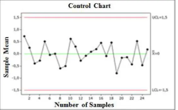
In summary, a control chart is a progressive graphic representation of a quality characteristic of interest (attribute or variable) or a statistic calculated from observed samples in a process that is periodically collected over time using the following reference lines:
UCL (upper control limit) = μD +dσD
CL (center line) = μD
LCL (lower control limit) =μD - dσD
where D is a statistic associated with a quality characteristic, d is a predetermined constant, and μD and σD are the mean and the standard deviation of D, respectively.
If the value of the statistic D is recorded within the control limits, the process is said to be under statistical control (no action has to be taken); otherwise, the process is said to be out of control (actions should be taken, such as searches for specific causes, stoppages of production, etc.).
It is typically assumed that items are produced one by one and samples of fixed size n are collected at regular intervals of duration h. The design of a control chart is completely by determining the values of n, d and h, adopting both statistical and economic criteria. Statistical criteria are associated with the probability of a false alarm or with the average number of samples after deviation occurs until its detection, while economic criteria seek to optimize an objective-function usually associated with operational costs (inspection, false alarm, adjustment, rework, etc.) per produced unit.
Figure 1 – Example of a control chart for monitoring the process mean.
The literature shows that Shewhart-type control charts are efficient for detecting the occurrence of large deviations relative to the target value (GOLDSMITH and WHITFIELD, 1961; CHAMP and WOODALL, 1987; MONFARED and LAK, 2013). To detect the occurrence of small deviations from the target value, EWMA-type and CUSUM-type control charts are more efficient and they are recommended to be used as they take into account past data in the decision-making process (MONTGOMERY, 2005; REYNOLDS JR and STOUMBOS, 2010).
However, in practice, there is typically interest in monitoring more than one quality characteristic. Therefore, multivariate control charts are developed in which the stability of several characteristics is assessed through a single chart – taking into account the structure of dependence among the p characteristics – instead of drawing separate control charts for each characteristic of interest. Literature reviews on multivariate control charts may be found in Alt and Smith (1988) and Bersimis, Psarakis, and Panaretos (2007). There are two common types of multivariate control charts; one monitors the stability of the vector of means and the other monitors the stability of the variance-covariance matrix. Considering that, a sample of size n is taken at regular intervals and from each sampled item, p characteristics are collected, the Hotelling’s T2 chart is typically used to monitor the stability of the vector of means. The statistic calculated and used in the T2 control chart is given in (2):
(2)
where is the vector of the sample mean of the p characteristics, , is the
vector of the mean (target value) of p quality characteristics; is the variance-covariance matrix of p quality characteristics; and the lower control limit (LCL) and
values are above the UCL, the process is said to be out of control and corrective actions should be taken.
To monitor the variance-covariance matrix, two types of charts may be used. One is based on the W statistic expressed in (3):
(3)
where S is the sample variance-covariance matrix, tr(.) denotes the trace of matrix (.), n is the sample size, and p is the number of monitored quality characteristics; |A| denotes the determinant of the matrix A. LCL and UCL are equal to zero and
, respectively. The other chart is constructed by utilizing the
generalized variance |S|, where |S| is the determinant of the sample variance-covariance matrix. In the case of p=2, it is known that follows
a Chi-Square distribution with (2n-4) degrees of freedom. In the case of p >2, using asymptotic properties of |S|, control charts can be created using
as control limits with
; ; (4)
;
(6)
In the case of processes, which behaviors are not known or are still in the
development stage, i.e., the parameters are unknown, unbiased and consistent estimators may be used in their place.
3. DATA ANALYSIS
For the geodesic auscultation of a specific dam, 77 distance measurements from pillars (fixed positions) to other positions (target points) were carried out sequentially over five epochs. These distances should (supposedly) vary little over time, and the variation measured by the residuals, should be small and random. The nominal accuracy of the equipment used in the measurement of the distances and the distribution of the targets in the dam are left undisclosed due to confidentially.
A LSM is proposed to adjust the distances to the model and the standard residual should (hopefully) follow a standard normal distribution mean equal zero and variance equal 1). For more details, see Gemael (1994).
To test the null hypothesis whether the standardized and raw residuals follow a normal distribution, the Anderson-Darling test is applied. Table 1 displays the p-values where Ri and Zi represent the raw and standardized residuals of the i-th
survey campaign, respectively. The null hypothesis is rejected to all raw residuals as also for the standardized residuals of the first and third survey campaigns
Table 1 – Descriptive level of the Anderson-Darling test. Variable p-value Variable p-value
Z5 0.227 R5 0.051
Z4 0.378 R4 0.094
Z3 <0.005 R3 <0.005
Z2 0.195 R2 0.105
Z1 0.006 R1 <0.005
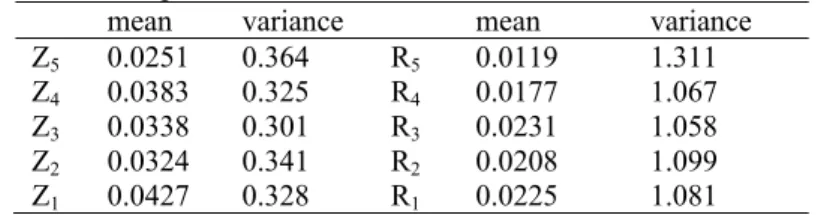
Table 2 shows the sample means and variances of the raw and standardized residuals of the 5 survey campaigns. According to it, the null hypothesis of the zero mean is not rejected for both the raw and standardized residuals.
Table 2 – Sample Mean and Variance of the raw and standardized residuals.
mean variance mean variance
Z5 0.0251 0.364 R5 0.0119 1.311
Z4 0.0383 0.325 R4 0.0177 1.067
Z3 0.0338 0.301 R3 0.0231 1.058
Z2 0.0324 0.341 R2 0.0208 1.099
Z1 0.0427 0.328 R1 0.0225 1.081
Table 3 shows the statistic values that are used to test the null hypothesis: the variance is equal one. It can be concluded that the null hypothesis is rejected for all standardized residuals. The rejection region with a type I error equal to 5% is [53.782; 101.999].
Table 3 – Statistic Values.
Statistic Statistic
Z5 27.694 R5 99.636
Z4 24.730 R4 81.092
Z3 22.868 R3 80.408
Z2 25.924 R2 83.524
The rejection of the null hypothesis (normal distribution) may indicate that there are gross errors (outliers) in the measurements (because of the parameters – particularly, the standardized residuals that seem to be inconsistent with the measured values) or that the fitted model can be equivocal. In this sense, the multivariate control charts are used to identify the unfit points by comparing jointly different survey campaigns in a single chart.
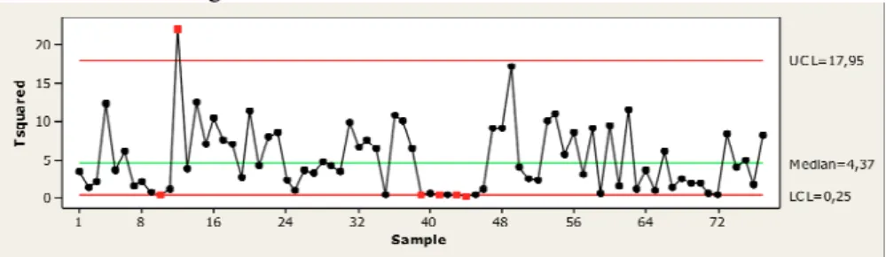
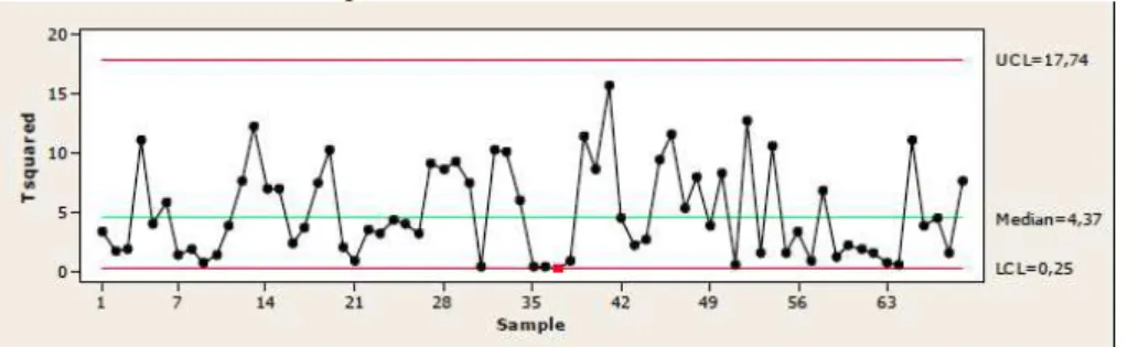
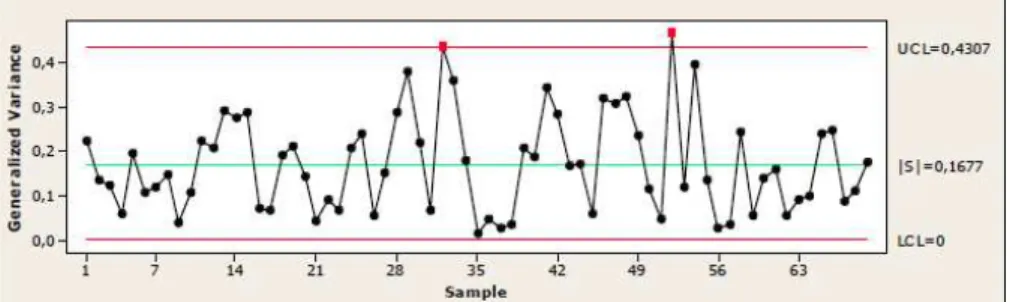
Figures 2A and 2B represent the T2 control charts of the standardized residuals and the raw residuals, respectively. Similarly, Figures 3A and 3B show the generalized variance control charts of the standardized residuals and the raw residuals, respectively.
Figure 2A - T2 control chart - standardized residuals.
Figure 2B - T2 control chart - raw residuals.
Figure 3B - Generalized Variance control chart - raw residuals.
There are several data points outside the control limits in both Figures 2A-2B, as also in Figures 3A-3B. These data points may have led to the rejection of the previously tested null hypotheses.
For processes in which the behaviors are unknown or in the development stage (i.e., unknown parameters), the values observed are typically removed – if they are outside of the control limits – to obtain more stable parameter estimates. With this aim, samples 10, 12, 39, 41, 43 and 44 (as a function of the T2 control charts) and observations 12, 14 and 20 (as a function of the generalized variance control chart) are excluded of the analysis.
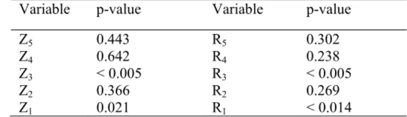
New Anderson-Darling tests are submitted for the remaining data and p-values are summarized in Table 4. Note that there is a significant improvement in the results and, in particular, for the raw residuals. However, both the raw and the standardized residuals of the third and first survey campaigns still do not follow a normal distribution.
Table 4 – P-values of the Anderson-Darling test– after exclusion the data points outside the control limits.
Variable p-value Variable p-value
Z5 0.443 R5 0.302
Z4 0.642 R4 0.238
Z3 < 0.005 R3 < 0.005
Z2 0.366 R2 0.269
Z1 0.021 R1 < 0.014
Figure 4A - T2 control chart - standardized residuals after exclusion of the data points outside the control limits.
Figure 4B – Generalized Variance control chart – standardized residuals after exclusion of the data points outside the control limits.
The stability of both the mean and the variance are shown in Figures 4A-4B. According to the preliminary analysis, data from the survey campaign 3 do not follow the normal distribution. These data are excluded because one of the assumptions to the use of these control charts is data normality. However the exclusion of data from survey campaign 3 to redraw the new control charts provided insignificant effect, as shown in Figures 5A-5B.
Figure 5A - T2 control chart - standardized residuals after exclusion of the data points from survey campaign 3.
Figure 5B – Generalized Variance control chart – standardized residuals after exclusion of the data points from survey campaign 3.
4. CONCLUSIONS AND RECOMMENDATIONS
This study proposed a method for monitoring multi-temporal data derived from geodesic survey campaigns by applying multivariate control charts. This quality tool has usually been employed to monitor production processes in industrial fields and, its use has expanded to include other areas of research, than production processes, such as public health, marketing, services.
The proposed method is simple and generates additional information beyond that obtained from traditional tests as it enables the analysis of individual survey campaigns associated with a temporal approach relative to multiple survey campaigns.
ACKNOWLEDGEMENTS:
The authors would like to thank the Department of Transport Engineering of the Polytechnic School of the University of São Paulo for the opportunity provided to conduct this study. The authors would like to acknowledge the National Research Council - Conselho Nacional de Pesquisa – CNPq for the support provided to the researchers.
REFERENCES
ALT, F. B.; SMITH, N. D. Multivariate process control. Handbook of Statistics, Eds P. R. Krishnaiah and C. R. Rao, Elsevier, Amsterdam, vol. 7, p. 333-351, 1988.
ARANTES, A.; CARVALHO, E. S.; MEDEIROS, E A. S.; FARHAT, C. K.; MANTESE, O. C. Use of statistical process control charts in the epidemiological surveillance of nosocomial infections. Revista de Saúde Pública, vol. 37, nº 6, p. 768-774, 2003.
BENNEYAN,J. C.; LLOYD, R. C.; PLSEK, P. E. Statistical process control as a tool for research and healthcare improvement. In: Quality and Safety Health Care, vol. 12, p. 458-464, 2003.
BERSIMIS, S.; PSARAKIS, S.; PANARETOS, J. Multivariate Statistical Process Control Charts: An Overview. Quality and Reliability Engineering International, vol. 23, p. 517–543, 2007.
CASPARY, W.F. (ed. By Jean M Rueger) Concepts of Network and Deformation Analysis. Kensington School of Surveying. The University of New South Wales, 1987.
CASPARY, W. F.; HAEN, W.; BORUTTA, H. Deformation analysis by statistical methods. Technometrics, vol. 32, nº 1, p. 49-57, 1990.
CHAMP, C. W.; WOODALL, W. H. Exact results for Shewhart control charts with supplementary runs rules. Technometrics, vol. 29, nº 4, p. 393-399, 1987. DENLI, H. H.; DENIZ, R. Global congruency test methods for GPS networks.
Journal of Surveying Engineering, vol. 95, p. 95-98, 2003.
GEMAEL, C. Introdução ao ajustamento de observações. Aplicações geodésicas
[Introduction to the fit of observations. Geodetic Applications]. Ed. UFPR. 1994.
GILES, D. E. A. A. Saddlepoint Approximation to the Distribution Function of the Anderson-Darling Test Statistic. In: Econometrics Working Paper EWP 0005. ISBN 1485-6441. Department of Economics, University of Victoria, B.C., Canada. April, 2000.
GOLDSMITH P. L.; WHITFIELD, H. Average run lengths in cumulative chart quality control schemes. Technometrics, vol. 3, nº 1, p. 11-20, 1961.
GUSTAFSON, T.L. Practical risk‐adjusted quality control charts for infection control. American Journal Infection Control, vol. 28, nº 6, p. 406-414, 2000. KANO, M.; NAKAGAWA, Y. Data-Based Process Monitoring, Process Control,
and Quality Improvement: Recent Developments and Applications in Steel Industry. Computers & Chemical Engineering, vol. 32 (1 – 2), p. 12-24, 2008. KULLAA, J. Damage detection of the Z24 bridge using control charts. Mechanical
Systems and Signal Processing, vol. 17, nº 1, p. 163-170, 2003.
MaCCARTHY, B.L.; WASUSRI, T. A review of non-standard applications of statistical process control (SPC) charts. International Journal of Quality and Reliability Management, vol. 19, nº 3, p. 295-320, 2002.
MAROTTA, G. S.; FRANÇA, G. S.; MONICO, J. F. G.; FUCK, R. A. Strains arising by seismic events in the SIRGAS-COM network region. Journal of Geodetic Science, vol. 3, nº 1, p. 12-21, 2013.
MARSHALL, C.; BEST, N., BOTTLE, A.; AYLIN, P. Statistical issues in the prospective monitoring of health outcomes across multiple units. Journal of the Royal Statistical Society: Series A, vol. 167, part 3, p. 541–559, 2004. MOHAMMED, M. A.; WORTHINGTON, P.; WOODALL, W. H. Plotting basic
MONFARED, M. E. D.; LAK, F. Bayesian estimation of the change point using
X
control chart. Communications in Statistics – Theory and Methods, vol. 42, p. 1572-1582, 2013.
MONTGOMERY, D. C. Introduction to Statistical Quality Control. 5th edition, John Wiley & Sons, Inc., 2005.
NIEMEIER, W. Statistical test for detecting movements in repeatedly measured geodetic networks. Tectonophysics, vol. 71, p. 335-351, 1981.
NING, X; SHANG, Y.; TSUNG, F. Statistical process control techniques for service processes: a review. In: ICSSSM International Conference on Service Systems and Service Management, p. 927- 931, 2009.
POPE, A. The statistics of residuals and the rejection of outliers. In: NOAA TR-NOS
65, NGSI, 1976.
REYNOLDS JR. M. R.; STOUMBOS, Z. G. Robust CUSUM charts for monitoring the process mean and variance. Quality and Reliability Engineering International, vol. 26, nº 5, p. 453-473, 2010.
SEVILLA, M. J.; GIL, A. J.; ROMERO, P. Adjustment of the first order gravity net
in Spain. Física de la Tierra, nº 2, Ed. Univ. Compl. Madrid, p. 149-203, 1990.
STEPHENS, M. A. EDF statistics for goodness of fit and some comparisons.
Journal of the American Statistical Association, vol. 69, p. 730-737, 1974. WOODALL, W.H. The Use of Control Charts in Health-Care and Public-Health
Surveillance. Journal of Quality Technology, vol. 38, nº 2, p. 89-104, 2006.