A Rough Sets based modified Scatter Search algorithm for solving 0-1 Knapsack problem

(1)

Decision Science Letters 4 (2015) 425–440 Contents lists available at GrowingScience

Decision Science Letters

homepage: www.GrowingScience.com/dsl

A Rough Sets based modified Scatter Search algorithm for solving 0-1 Knapsack problem

Hassan Rezazadeh*

Department of Industrial Engineering, University of Tabriz, Tabriz, Iran

C H R O N I C L E A B S T R A C T

Article history:

Received December 10, 2014 Received in revised format: January 4, 2015

Accepted February 20, 2015 Available online

February 24 2015

This paper presents a new search methodology for different sizes of 0-1 Knapsack Problem (KP). The proposed methodology uses a modified scatter search as a meta-heuristic algorithm. Moreover, rough set theory is implemented to improve the initial features of scatter search. Thereby, the preliminary results of applying the proposed approach on some benchmark dataset appear that the proposed method was capable of providing better results in terms of time and quality of solutions.

Discrete optimization 0-1 Knapsack problem Rough sets theory Scatter search algorithm

1. Introduction

0-1 Knapsack Problem (0-1 KP) is a special case of general 0-1 linear problem in which the allocation of items to a knapsack is discussed. Knapsack problems appear in real-world decision-making processes in a wide variety of fields such as production, logistics, distribution and ﬁnancial problems (Marchand et al., 1999; Kellerer et al., 2004; Gorman & Ahire, 2006; Wascher & Schumann, 2007; Granmo et al., 2007; Nawrocki et al., 2009; Vanderster et al., 2009). Dantzig (1957) is believed to be the first who introduced the knapsack problem and proved that the complexity of this problem is NP-hard (Garey & Johnson, 1979). There are literally many practical applications for knapsack problem and it has become the object of numerous studies and a great number of papers have been proposed for solving this problem. In this problem, different items with various profits (p) and weights (w) are considered. There is also capacity limit in knapsack problem (C). The general KP model is a binary problem, stated as follows:

* Corresponding author.

(2)

n

i i i 1 n

i i i 1

i

max f (x) p x

subject to w x C

x {0,1} , i 1,..., n

=

= =

≤

∈ ∀ =

∑

(1)

In this problem xi is a binary variable, which is one, when the item i is chosen and zero, otherwise.

In this paper, a scatter search methodology evolved by Rough Sets theory to solve 0-1KP for problems in different sizes, is developed. The proposed model of this paper takes advantage of rough sets theory, which relies on Meta models to reduce the objective function evaluations.

The rest of the paper is organized as follows: in the next section, the literature review on 0-1KP is presented. Brief description of scatter search and rough sets theory are presented in section 3. Section 4 describes the proposed RSSS approach for optimization of 0-1KP in more detail and experimental results are presented in section 5. Finally, the advantages of the proposed structure, conclusions, and possible future work are discussed in section 6.

2. Literature review

(3)

Regarding these variations, it is clear that each researcher has studied the KP from different aspects. For instance, there could be environmental or social concerns as well as economic goals. Moreover, in some cases, KP problem can be studied in the context of portfolio and logistics problems. Silva et al. (2006) proposed a scatter search method for bi-criteria 0-1KP.Silva et al. (2006) stated the core concept in bi-criteria 0-1 KPs. Beausoleil et al. (2008) suggested multi-start and path re-linking methods to deal with multi objective KPs. Taniguchi et al. (2009) applied a virtual pegging approach to the max–min optimization of the bi-criteria KP. Kumar and Singh (2010) proposed an assessing solution quality of multi-objective 0-1 KP using evolutionary and heuristic algorithms. Sato et al. (2012) applied Variable Space Diversity, crossover and mutation in multi objective evolutionary algorithm for solving many-objective KPs. Lu and Yu (2013) proposed an adaptive population multi many-objective quantum-inspired evolutionary algorithm for multi objective KPs.

3. Brief conceptions of scatter search and rough sets theory

3.1Scatter search

Glover (1998) is believed to be the first who presented Scatter Search. Unlike other similar algorithms, Scatter Search uses results to search in solution space purposefully and deterministically. This algorithm, directs vectors with a set of solutions called Reference Set (RefSet) and obtains optimal solutions from the prior solutions. RefSet includes a set of solutions that have both variety and quality that an algorithm needs them for covering the whole solution space for getting near the optimum solution (Glover, 1998).

Scatter Search methodology has been best known for its flexibility in solving variety of problems. Even the internal sub methods of it are very flexible. Consequently, this procedure can be implemented to solve different problems in various scales. In this section, we propose a general description of Scatter Search steps, but these five steps will be adapted to the proposed problem in the next sections. Note that the complexities of these methods are being “changed” and not only “reduced or expanded” according to the problem. The general descriptions of these steps are as follows:

1) Diversification Generation Method: Generates diverse solutions using a random (or a set of random) solutions called seed solutions.

2) Improvement Method: Transforms the diverse solutions produced in the prior method into more qualified solutions (neither the input nor the output solutions are required to be feasible, but it is rather that outputs be feasible)

3) Reference Set Update Method: keeps the “best” solution in the RefSet (in the first place and during the algorithm). Meaning that, the “best” solution satisfies both quality and diversity of solutions.

4) Subset Generation Method: Produces a subset of RefSet as a basis for Combination Method. 5) Solution Combination Method: transforms the members of subset generated in the prior step to

new solutions by combining solution vectors.

3.2Rough sets theory

Rough Sets theory is a new mathematical approach to imperfect knowledge that is proposed by Pawlak (1992) and works on vague and imprecise environments. The theory works on the notion of sets and the relationships among them. The Rough Sets theory has its basis on the information that we have about every member of universe, the collection of objects we am interested in, and tries to present a way to transform data to knowledge and gives us a useful method for discovering hidden patterns in the raw data (Mrozek, 1992).

(4)

of “upper and lower approximations of set” and set modeling (Slowinski, 1992). In this method, the superfluous data in aspect of reasoning will be removed and the indispensable data will be on board to derive the decision rules from them. We now describe the fundamental concepts of Rough Sets theory that is used in the proposed methodology in this paper.

3.2.1 Relational Systems (Knowledge Base)

Suppose that there is a finite set U ≠ ∅(the universe) of subjects, we are observing or interested in. Any subset X ⊆U of the universe is called a concept or a category in U and any family of concepts in U will be referred to knowledge about U. If R is an equivalence relation over U, then by U R/ _{, we}

mean that family of equivalence classes of R referred to as categories of R and [x]_R denotes a category

in R containing an elementX ⊆U.

3.2.2 Indiscernibility relation

If P⊆R and P≠φ then intersection of all equivalence relationships of P is also an equivalence relation, which is shown by IND P( ) (indiscernibility relation over P); so we have

( )

[ ]

_{IND P}

[ ]

_R

R P

x

∈

=



_. ₍₂₎

Thus U /IND P( )or in short U /P, denotes knowledge associated with the family of equivalence

relations P, called P-basic knowledge about U. In fact, P-basic categories have those of basic properties of the universe, which can be expressed employing knowledge P.

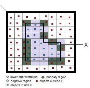
3.2.3 Approximation of sets

As we have demonstrated before, some categories cannot be expressed exactly by employing available knowledge. By Rough Sets theory, we are able to make an approximation of a set by other sets. These sets are called lower and upper approximations. The lower and upper approximations can be presented in an equivalent form as follows,

} ]

[ :

{x U x X

X

R = ∈ R ⊆

} X ]

x [ : U x { X

R = ∈ _R  ≠

φ

X R X R ) X (

BN_R = −

(3)

The set RX is the set of all elements of U, which can be certainty classified as elements of X, in

knowledge R. The Set

R

X

is the set of elements of U,which can be possibly classified as elements of

X, employing knowledge R and Set BN_R(X) is the set of elements, which cannot be classified to X or

to -X having knowledge R.

(5)

Fig. 1. Schematic overview of approximations

4. Proposed algorithm

Scatter Search is a meta-heuristic algorithm that applies a global search in solution space with a set called RefSet. Three methods of five general scatter search methods depend on the type and complexity of the problem including Diversification Generation Method, Improvement Method, and Combination Method. Therefore, it is essential to introduce the problem I am going to solve so that I can justify three methods referred.

4.1Diversification generation method

As mentioned before, in Scatter Search methodology first step is to generate a set of diverse solution with a random mechanism. To this end, we applied a systematic mechanism proposed by Glover (1977) to produce a diverse set of binary vectors. First consider h =2, 3,...,h_max, which h_max ≤ −n 1, which must be assigned a value of one or a set of seed solutions to build up the other answers on it. Our seed solution is a vector that picks zero for every array of it. “div” number of random solutions is being produced here and they are presented by x'that:

'

1 hk

1

1 hk

x

₊

= −

x

₊ for k 0,1,..., ([ ] 1)n

h

= − (4)

As it can be noticed, the proposed method creates “

2

div

” of diverse solutions and other “

2

div

” will be

the complement of these solutions so that:

'' '

1

i i

x

= −

x

. (5)

Now, we have our diverse solutions that they might be feasible or not. Finally, in the last step of this method, we make them feasible by a random technique. We randomly choose variables that accepted one and switch them to zero until the solution becomes feasible. Therefore, the idea of random solution creation in Diversification Generation Method will stay untouched.

4.2. Improvement method

(6)

we just used objective function evaluation for computing ratio as below which x_i represents the decision variable that picks 0 or 1 in the diverse solutions.

{ | 1}

i i

A = x x = , B_i ={ |x x_i =0}

Ratio(i)

Ai Bi

i

f

wco

−

=

(6)

i

A

f

is the average of objective function in “

2

div

” of solutions that have a better objective value when

the i’th decision variable picks 1.

i

B

f

is the average of objective function in “

2

div

” of solutions that have a better objective value when

the i’th decision variable picks 0.

�� represents weight coefficient or the coefficient of i’th variable in constraint.

Consequently, we have a ratio for each decision variable, which helps us decide about every variable. However, the procedure goes like this that in first step in case of infeasible solutions; the proposed study sorts the ratios of variable and variables with values of one with the least ratio transform to zero and this procedure continues until the solutions become feasible. In the next step, variables with value of zero with the most ratio are switched to one. The feasibility is required in both conditions.

4.3 Reference Set Update Method

This method first sorts the solutions according to their objective function values. As mentioned in general scatter search description, RefSet is a set of “b” (b = +b₁ b₂) solutions that b₁ number of them

are solutions with high quality and b₂ number of solutions are the most diverse solutions in solution

space. Because of sorting these solutions, b₁is updated with the solutions that have the best objective

function value. In this step, the ratio is updated based on the new members ofb₁.Next step is to update

2

b . For maximum diversity according to high quality solutions; we define a distance function that calculates the “distance” of two solutions and by using the function. Regarding these values, we will be able to figure out which solutions in population have the maximum distance from the members of

1

b . The proposed study calculates the minimum distance of every solution in population with the

members of b₁and solutions that have the maximum of minimum distances will be chosen to fillb₂.

4.4. Subset generation and Combination method

We simply choose two of solutions using permutation for combining in next method. Suppose we have two solutions from RefSet selected by Subset generation method. For creating new solutions, we assign a value of 1 for variables that have the value of 1 in both picked solutions and pick 0 or 1 randomly for the rest of variables. To make new solution, the feasibility is a required condition. In the next step, the Improvement Method improves generated solutions and their objective function values will be compared with the members of b₁ and in the case of improvement in new solutions, the replacement

will be settled with the worst member of b₁. For diverse solutions, we compare the distance of new

solutions from the b₁with the temporary members of b₂ and in case of improvement in diversity, new solutions will be substituted. As it can be noticed, this method is a loop and the algorithm ends when b

(7)

4.5Pop size update with rough sets theory

As mentioned before, if b is remained unchanged, the population will be reproduced and all of methods will be repeated on new set of solutions in population but in case of speed and quality of obtained solutions, the population update can be very important. To this end, we use Rough Sets Theory for updating Population and the idea is described as follows.

Suppose that we have an n sized problem, meaning the objective function has n variables, say

1, 2,..., n

x x x . After a loop, we have an imprecise knowledge about every variable’s effect in objective function and the knowledge is obtained from the best solutions in b1, so in Rough Sets Theory terms,

if my universe is U ={ ,x x₁ ₂,...,x_n} that classifies b1members to two equivalent classes, respectively,

variables which picked value of one in b1, and variables which picked value of zero in b1. Therefore,

for every solution we have a Relational System as follows,

( , )

i i

K = U R i =1, 2,...,b₁, (7)

where U R/ _idenotes knowledge associated with the family of equivalence relationsR_i, called R_i-

basic knowledge about U inK_i . Equivalence classes of R_iare called basic categories (concepts) of

knowledgeR_i. In other words, the equivalence relations of R_i are the basic concept of universe that

can be represented inR_i. To illustrate the idea we will serve an example.

Consider that we have 10 decision variables (n=10),b₁=3which is as follow,

1

Refset ={0,1,1,1, 0, 0, 0, 0,1,1} (8)

2

Refset ={1, 0,1,1, 0, 0, 0, 0, 0, 0}

3

Refset ={0,1,1,1,1, 0, 0, 0,1, 0}

By classification of (1 or 0), we define three equivalence relationsU R/ ₁, U R/ ₂ and U R/ ₃ that have the following classes,

1 2 3 4 9 10 1 5 6 7 8

/ {{ , , , , },{ , , , , }}

U R = x x x x x x x x x x , (9)

2 1 3 4 5 2 6 7 8 9 10

/ {{ , , , },{ , , , , , }}

U R = x x x x x x x x x x ,

3 2 3 4 5 9 1 6 7 8 10

/ {{ , , , , },{ , , , , }}

U R = x x x x x x x x x x .

These are elementary categories (concepts) in the knowledge basedK =( ,{U R R R₁, ₂, ₃}). Theoretically, basic concepts are sets that are intersections of elementary categories, so we have

1 2 3

{ , , }

S = R R R . According to the set of variables that values are one we have:

{1,1,..,1}

X = (10)

1 2 3 3 4

{ | [ ]_S } {[1]_R [1]_R [1] } {_R , }

S X = x ∈U x ⊆X = ∩ ∩ = x x

1 2 3 1 2 3 4 5 9 10

{ :[ ]_S _R [1]_R [1] } { ,_R , , , , , }

S X = x ∈U x ∩X ≠ ∅} = {[1] ∪ ∪ = x x x x x x x

6 7 8

( ) { , , }

S

NEG X = −U S X = x x x

(8)

S. Now we can calculate NEG_S(X ) {= x₆,x₇,x₈}that refers to variables, which cannot be a member of set X, in the knowledge of S.

We use this procedure for updating Population. First, we put the b members of RefSet in new Population, then by applying rough Sets Theory data reasoning on Refset₁, we calculate the R X and

pick value of one for the members of R X and oppositely pick value of zero for the members of

( )

S

NEG X . Other variables, in terms of rough Sets Theory, are calledBOUNDRY_S(X ) pick 0 or 1 with a random procedure. Now we have a new Population that the whole Scatter Search must be implemented on.

5. Experimental results

We have coded the proposed Rough Sets based modified Scatter Search (RSSS) algorithm in Matlab on an Intel Core i3, 1.736 Ghz processor with 4Gb RAM. To evaluate the performance of RSSS algorithm, two sets of Ill-known benchmark problems in the 0-1KP literature have been considered:

(1) Small sizes: The data set consists of ten collected instances [f1-f10] from Zou et al.(2011) with

number of items ranging from 4 to 23 and ten instances [f11-f20] from Kulkarni and Shabir (2014) with

number of items ranging from 30 to 75.

(2) Large-scale sizes: The data set consists 96 problems from Pisinger (1995) with a variety of variable sizes (n= 100, 300, 1000, 3000). To cover all kinds of possible conditions, the problems have been categorized into different classes. We have run this algorithm 20 independent times for each instance from Zoa data and 10 independent times for each instance from Pisinger data.

5.1. Results of small and medium size problems

The first data set under study includes small-scale problems. The proposed model can be optimally solved within noticeable time for small instances. Thus, to solve these problems, we have considered a global optimum value of objective function (GOV) obtained from branch and bound algorithm (B&B) to compare with the solution of the RSSS algorithm.

The following ranges of parameter values from the scatter search literature were tested

pop_size=[10,100], b=[3-21], b1=[2-14], b2=[1-7]. Based on experimental results, Table 1 shows the

best parameter settings.

Table 1

RSSS parameter settings

Parameter Pop_size b b1 b2

Value 20 18 12 6

To judge the effectiveness of the proposed algorithm, the following three criteria were evaluated (Rezazadeh et al., 2011):

1. BS=[(BSRSSS-GOV) /GOV]*100: gap between GOV and best solution obtained from RSSS (BSRSSS).

2. MS=[(MSRSSS-GOV) /GOV]*100: gap between GOV and mean solution obtained from ten repeated

times of RSSS (MSRSSS).

(9)

The obtained results and comparison of B&B and RSSS algorithms corresponding to the 20 problems are shown in Table 2.

Table2

The obtained results and comparison from B&B and RSSS runs

NO. Problem info. B&B RSSS RSSS GAP

Objects Capacity GOV TBB BSRSSS MSRSSS TBSRSSS BS % MS % (|BSRSSS-MSRSSS|)%

1 10 269 295 .12 295 295 1.26 0 0 0

2 20 878 1024 .04 1024 1018 1.32 0 -.59 .59

3 4 20 35 .03 35 35 1.20 0 0 0

4 4 11 23 .03 23 23 1.21 0 0 0

5 15 375 481.069 .18 481.069 480.25 1.14 0 -.17 .17

6 10 60 52 .14 52 51 1.25 0 -1.92 1.92

7 7 50 107 .04 107 105 1.25 0 -1.86 1.86

8 23 10000 9767 .18 9767 9767 1.27 0 0 0

9 5 80 130 .03 130 130 1.24 0 0 0

10 20 879 1025 .45 1025 1019 1.29 0 -.58 .58

11 30 577 1437 .156 1437 1437 1.28 0 0 0

12 35 655 1689 .0624 1689 1686 1.28 0 -.18 .18 13 40 819 1821 .0156 1821 1819 1.34 0 -.11 .11

14 45 907 2033 .0312 2033 2033 1.28 0 0 0

15 50 882 2440 .0312 2440 2438 1.31 0 -.08 .08

16 55 1050 2440 .0312 2440 2651 1.92 0 0 0

17 60 1006 2917 .0312 2917 2917 2.33 0 0 0

18 65 1319 2818 .0624 2818 2817 2.29 0 -.04 .04 19 70 1426 3223 .078 3223 3221 2.29 0 -.06 .06

20 75 1433 3614 .0312 3614 3614 2.31 0 0 0

Avg. 0 -.28 .28

We have also compared the performance of the RSSS algorithm with recently proposed algorithm including Cohort Intelligence Algorithm (CI) (Zhang, 2013), Shuffled Frog Leaping Algorithm (MDSFLA) (Bhattacharjee & Sarmah, 2014), Novel Global Harmony Search Algorithm (NGHS) (Zou et al., 2011), Quantum Inspired Cuckoo Search Algorithm (QICSA) (Layeb, 2011), Quantum Inspired Harmony Search Algorithm(QIHSA) (Layeb, 2013). The detail results are listed in Table 3.

In Table 3, the first column symbolizes the name for each instance; the second column shows the information of instance; the third column lists the global optimum solution (GOV) and the remaining columns describe the computational results of RSSS, CI, MDSFLA, NGHS, QICSA and QIHSA respectively.

Table 3

Results Comparison from CI, MDSFLA, NGHS, QICSA, QIHSA and RSSS

No. Problem info. GOV RSSS CI MDSFLA NGHS QICSA QIHSA

objects capacity

f1 10 269 295 295 295 295 295 295 340

f2 20 878 1024 1024 1024 1024 1024 1024 1024

f3 4 20 35 35 35 35 35 35 35

f4 4 11 23 23 23 23 23 23 23

f5 15 375 481.07 481.07 481.07 481.07 481.07 481.07 481.07

f6 10 60 52 50 51 52 50 52 52

f7 7 50 107 107 105 107 107 107 107

f8 23 10000 9767 9767 9759 9767 9761 9767 9767

f9 5 80 130 130 130 130 130 130 130

f10 20 879 1025 1025 1025 1025 1025 1025 1025

f11 30 577 1437 1437

f12 35 655 1689 1689

f13 40 819 1821 1816

f14 45 907 2033 2020

f15 50 882 2440 2440

f16 55 1050 2651 2643

f17 60 1006 2917 2917

f18 65 1319 2818 2814

f19 70 1426 3223 3221

(10)

5.2. Results of Large scale problems

The second data set investigated is associated with Pisinger data (Pisinger 1995). We have compared the results of proposed RSSS algorithm with commercial software’s like OptQuest, Solver, Evolver and the methods proposed in Gortázar et al. (2010) called BinarySS and Pisinger (1995) called Expknp. In a similar vein, we have used the range of data sets as R = 100, 1000, 10000 and used Pisinger’s exact method, which uses the objective function coefficients as a best-known value solver. By solving the problems with various variable numbers (n) and proposed ranges (R), the number of feasible solutions in each method is shown in Table 4.

Table 4

Number of feasible solutions that solved

Method Number of feasible solutions Method Number of feasible solutions

OptQuest 96 Binary SS 96

Evolver 40 ExpKnp 96

Solver 47 RSSS 96

As far as the knowledge of researchers is concerned, one of the features of algorithm quality is the number of objective function evaluations that solver uses to find the best solution. In Table 5, the numbers of function evaluations for the problems in different sizes are proposed. It is obvious that by using the Rough Sets theory, the superfluous evaluations have been eliminated and there are a reasonable number of objective function evaluations.

Comparing to the last research in this field, there is a great progress in our results regarding the fact that we used only one Diversification Generation Method and one Combination Method while in Gortázar et al. (2010), three Diversification Generation Methods and seven Combination Methods were used and we obtained better results. Best-known values and results of commercial software such as OptQuest, Evolver, Solver and ExpKnap, Binary SS and RSSS algorithms are shown in Tables 6-17.

Table 6

n=100, R=100

Instance Best Known Value RSSS BinarySS ExpKnap OptQuest Evolver Solver

Strongly correlated 3352 3352 3332 3352 3265 3329 3322

3132 3132 3102 3132 3050 3094 3102 weakly correlated 3083 3083 3079 3083 3008 2957 3051

2945 2945 2942 2945 2873 2815 2917

Subset sum 2647 2647 2647 2646 2647 2647 2647

2583 2583 2583 2582 2583 2583 2583

Uncorrelated 4218 4218 4218 4218 4115 4214 4208

4149 4149 4149 4149 4089 3984 4099 Table 5

Number of function evaluations by RSSS

Type of data n Function evaluations

Strongly correlated

100 7708

300 27289

1000 41585

3000 36470

weakly correlated

100 18966

300 28611

1000 50247

3000 77496

Subset Sum

100 4607

300 4237

1000 3844

3000 3475

Uncorrelated

100 24945

300 65722

1000 104447

(11)

Table 7

n=100, R=1000

Strongly correlated 26692 26692 26682 26681 26551 26498 26527

24942 24942 24902 24940 24791 24902 24809 Weakly correlated 27992 27992 27950 27977 27533 27939 27718

27229 27229 27229 27166 26336 26984 27171 Subset sum 26347 26347 26347 26335 26347 26347 26347

24383 24383 24383 24372 24383 24383 24383 Uncorrelated 38795 38795 38795 38795 37979 38660 38680 Table 8

n=100,R=10000

252932 252932 252902 252713 252741 252788 252742 Weakly correlated 274437 274437 274227 274349 266623 274046 273005

274588 274588 274395 274588 268696 274108 272438 Subset sum 270847 270847 270847 270499 270836 270847 270846

258883 258883 258883 258864 258882 0 258876 Uncorrelated 423809 423809 423809 423809 420486 423777 418785

415239 415239 415239 414552 409984 0 411183 Table 9

n=300,R=100

9715 9715 9496 9715 9273 9368 9456 Weakly correlated 8550 8550 8527 8549 7899 8024 8325

8721 8721 8700 8720 8128 7940 8484

Subset sum 7492 7492 7492 7492 7492 7492 7492

7556 7556 7556 7556 7556 7556 7556

Uncorrelated 12059 12059 12009 12055 10104 11563 11610

12251 12251 12239 12250 10416 11492 11996 Table 10

n=300, R=1000

77356 77356 77266 77356 76862 0 76823 Weakly correlated 85278 85278 84978 85278 79683 83620 83038

77637 77637 77476 77630 71730 76091 75897 Subset sum 75242 75242 75242 75241 75241 75242 75242 76006 76006 76006 76005 76005 76006 76005 Uncorrelated 121294 121294 121072 121261 103405 109845 118037

120727 120727 117842 117922 102417 102498 114706 Table 11

n=300, R=10000

Strongly correlated 792840 792678 792525 792837 792243 0 792305

758876 758752 758675 758812 758183 758444 758310 Weakly correlated 838118 835319 833559 838005 772371 798541 820433

794763 791693 791465 794643 748288 754892 772016 Subset sum 796242 796242 796242 796221 796238 796238 796235

745006 745006 745006 744955 744973 744984 745004 Uncorrelated 1207003 1207003 1206852 1207003 1019380 1161232 1185688

1249781 1247645 1247645 1249687 1078371 0 1234197 Table 12

n=1000,R=100

Strongly correlated 32351 32201 30671 32351 30420 0 0

31977 31817 30327 31977 30072 30848 0 Weakly correlated 27511 27349 27343 27509 25176 0 0

27913 27710 27748 27913 25375 0 0 Subset sum 25099 25099 25099 25099 25094 25099 0

24637 24637 24637 24637 24636 24637 0 Uncorrelated 41024 40017 40011 41024 28081 34924 0

(12)

Table 13

n=1000, R=1000

266198 264359 264500 266188 242238 0 0 Subset sum 252399 252399 252399 252397 252098 252399 0

250987 250987 250987 250987 250951 0 0 Uncorrelated 407145 395677 395677 407129 293063 0 0

406291 396950 395878 406287 274276 0 0 Table 14

n=1000, R=10000

2503917 2503899 2502256 2503910 2501056 0 0 Weakly correlated 2697872 2669364 2684938 2697823 2465875 2573734 0

2681419 2665841 2664817 2681281 2453269 2555126 0 Subset sum 2502899 2502899 2502899 2502897 2502854 2502899 0

2509987 2509987 2509987 2509987 2509702 2509987 0 Uncorrelated 4124595 4011754 4003030 4124551 2776044 0 0

4101915 4009395 3994678 4101457 2945780 0 0

Table 15

n=3000,R=100

95462 94162 89752 95462 89324 90603 0 Weakly correlated 83588 82216 83070 83588 75553 77649 0

84163 83677 83677 84162 76130 78298 0

Subset sum 76159 76159 76159 76159 76055 0 0

74673 74673 74673 74673 74441 74673 0 Uncorrelated 123483 116963 116963 123482 76311 0 0

123401 116251 117053 123401 77843 0 0 Table 16

n=3000, R=1000

819621 816945 814554 819612 746590 0 0 Subset sum 752659 752659 752659 752659 748064 0 0

746123 746123 746123 746123 745705 746123 0 Uncorrelated 1216420 1153501 1153501 1216409 770998 914570 0

1216952 1157174 1156501 1216942 785440 0 0 Table 17

n=3000, R=10000

7449492 7449492 7443562 7449487 7434434 7443176 0 Weakly correlated 8196827 8196827 8149319 8196827 7471932 0 0

8195660 8195660 8151899 8195619 7452938 7656176 0 Subset sum 7532159 7532159 7532159 7532156 7531447 7532159 0

7465623 7465623 7465623 7465622 7423888 0 0 Uncorrelated 12216592 12216560 11525746 12216550 7843188 0 0

12363244 12363186 11788031 12363178 7791499 0 0

(13)

Table 18

The average GAP of several methods

Range n RSSS BinarySS OptQuest Evolver Solver

100 2.5 7.125 59.875 2083.125 22.5

100 300 44.625 71.875 745.75 8105.125 208.25

1000 320.5 694.75 4331.25 12644.625 26817

3000 2256 3150.25 15184.875 54680 94832

100 11.2875 13.1428 351.4285 14894.5 93.125

1000 300 306 478.375 6093.5 49766.875 1789.25 1000 3125.75 3516 37068.625 232242.5 296591.375 3000 16861.375 18086.5 130432.75 681741.5 889331.875

100 39.875 109.125 2884.25 84463 1682.625

10000 300 1028 1324.125 5906.375 657860.75 6953.375 1000 31422.5 32731.875 371297.25 1682679.25 2950386.25 3000 172928.375 171157.375 1310846.625 5099281.25 8858051.25

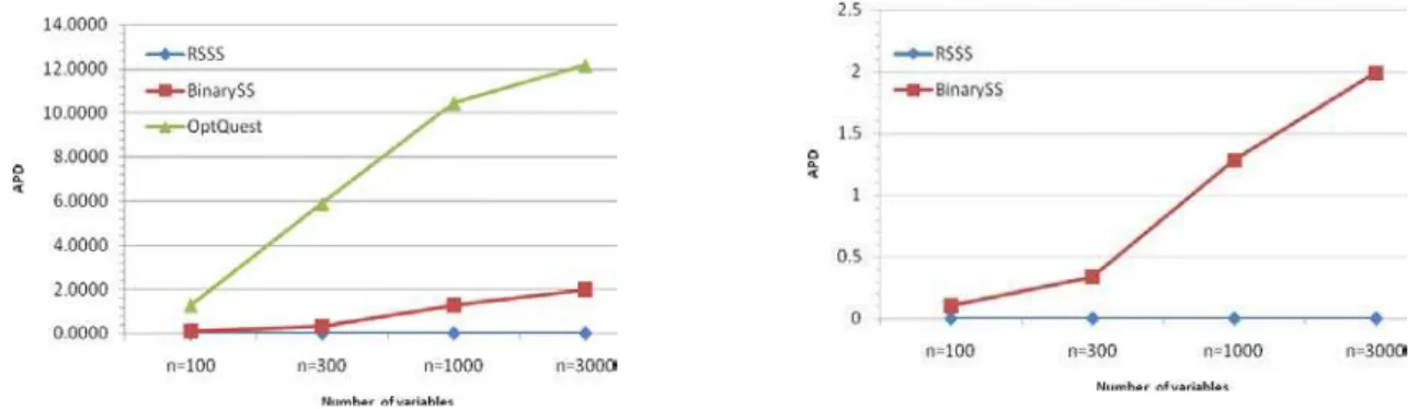
According to the results of Table 18, it is obvious that the three methods, RSSS, BinarySS, and OptQuest

have provided more qualified solutions. For comparing the efficiency of these methods, we have defined Absolute Percent Deviation (APD), which divides the GAP to the best-known value for each problem as follows,

100

GAP APD

Best known value

= × (11)

The results of Fig. 2 demonstrates the calculated APD for these three methods in various variable numbers. In fact, this figure shows the deviation of obtained solution by each method from the

best-known value, in which the efficiency of RSSS is obvious.

Fig. 2. The value of APD for each number of variables

6. Conclusions

(14)

Acknowledgement

The authors would like to thank the anonymous referees for constructive comments on earlier version of this paper.

References

Albano, A., & Orsini, R. (1980). A tree search approach to the M-partition and knapsack problems. The Computer Journal, 23(3), 256-261.

Archetti, C., Guastaroba, G., & Speranza, M. G. (2013). Reoptimizing the rural postman problem. Computers & Operations Research, 40(5), 1306-1313.

Bansal, J. C., & Deep, K. (2012). A modified binary particle swarm optimization for knapsack problems. Applied Mathematics and Computation, 218(22), 11042-11061.

Beausoleil, R. P., Baldoquin, G., & Montejo, R. A. (2008). Multi-start and path relinking methods to deal with multiobjective knapsack problems. Annals of Operations Research, 157(1), 105-133. Belgacem, T., & Hifi, M. (2008). Sensitivity analysis of the optimum to perturbation of the profit of a

subset of items in the binary knapsack problem. Discrete Optimization, 5(4), 755-761.

Bhattacharjee, K. K., & Sarmah, S. P. (2014). Shuffled frog leaping algorithm and its application to 0/1 knapsack problem. Applied Soft Computing, 19, 252-263.

Dantzig, G. B. (1957). Discrete-variable extremum problems. Operations research, 5(2), 266-288. Gary, M. R., & Johnson, D. S. (1979). Computers and Intractability a Guide to the Theory of

NP-Completeness. 1979. WH Freman and Co.

Glover, F. (1977). Heuristics for integer programming using surrogate constraints. Decision Sciences, 8(1), 156-166.

Glover, F., Laguna, M., & Marti, R. (2003). Scatter search and path relinking: Advances and applications. In Handbook of metaheuristics (pp. 1-35). Springer US.

Gorman, M. F., & Ahire, S. (2006). A major appliance manufacturer rethinks its inventory policies for service vehicles. Interfaces, 36(5), 407-419.

Gortázar, F., Duarte, A., Laguna, M., & Martí, R. (2010). Black box scatter search for general classes of binary optimization problems. Computers & Operations Research, 37(11), 1977-1986.

Granmo, O. C., Oommen, B. J., Myrer, S. A., & Olsen, M. G. (2007). Learning automata-based solutions to the nonlinear fractional knapsack problem with applications to optimal resource allocation. Systems, Man, and Cybernetics, Part B: Cybernetics, IEEE Transactions on, 37(1), 166-175.

Guler, A., Nuriyev, U. G., Berberler, M. E., & Nuriyeva, F. (2012). Algorithms with guarantee value for knapsack problems. Optimization, 61(4), 477-488.

Kellerer, H., Pferschy, U., & Pisinger, D. (2004). Knapsack problems. Springer Science & Business Media.

Kumar, R., & Singh, P. K. (2010). Assessing solution quality of biobjective 0-1 knapsack problem using evolutionary and heuristic algorithms. Applied Soft Computing, 10(3), 711-718.

Kulkarni, A. J., & Shabir, H. (2014). Solving 0–1 knapsack problem using cohort intelligence algorithm. International Journal of Machine Learning and Cybernetics, 1-15.

Layeb, A. (2011). A novel quantum inspired cuckoo search for knapsack problems. International Journal of Bio-Inspired Computation, 3(5), 297-305.

Layeb, A. (2013). A hybrid quantum inspired harmony search algorithm for 0–1 optimization problems. Journal of Computational and Applied Mathematics,253, 14-25.

Lasserre, J. B., & Thanh, T. P. (2012). A “joint+ marginal” heuristic for 0/1 programs. Journal of Global Optimization, 54(4), 729-744.

Lin, C. J., & Chen, S. J. (1994). A systolic algorithm for solving knapsack problems. International Journal of Computer Mathematics, 54(1-2), 23-32.

(15)

Lin, G., Zhu, W., & Ali, M. M. (2011). An exact algorithm for the 0–1 linear knapsack problem with a single continuous variable. Journal of Global Optimization, 50(4), 657-673.

Lu, T. C., & Yu, G. R. (2013). An adaptive population multi-objective quantum-inspired evolutionary algorithm for multi-objective 0/1 knapsack problems. Information Sciences, 243, 39-56.

Marchand, H., & Wolsey, L. A. (1999). The 0-1 knapsack problem with a single continuous variable. Mathematical Programming, 85(1), 15-33.

Martello, S., Pisinger, D., & Toth, P. (1999). Dynamic programming and strong bounds for the 0-1 knapsack problem. Management Science, 45(3), 414-424.

Mrozek, A. (1992). Rough sets in computer implementation of rule-based control of industrial processes. In Intelligent Decision Support (pp. 19-31). Springer Netherlands.

Martello, S., Pisinger, D., & Toth, P. (2000). New trends in exact algorithms for the 0–1 knapsack problem. European Journal of Operational Research, 123(2), 325-332.

Nawrocki, J., Complak, W., Błażewicz, J., Kopczyńska, S., & Maćkowiaki, M. (2009). The Knapsack -Lightening problem and its application to scheduling HRT tasks. Bulletin of the Polish Academy of Sciences: Technical Sciences, 57(1), 71-77.

Pisinger, D. (1995). An expanding-core algorithm for the exact 0–1 knapsack problem. European Journal of Operational Research, 87(1), 175-187.

da Cunha, A. S., Bahiense, L., Lucena, A., & de Souza, C. C. (2010). A New Lagrangian Based Branch and Bound Algorithm for the 0-1 Knapsack Problem.Electronic Notes in Discrete Mathematics, 36, 623-630.

Kaparis, K., & Letchford, A. N. (2010). Separation algorithms for 0-1 knapsack polytopes. Mathematical programming, 124(1-2), 69-91.

Pawlak, Z., (1992).Rough set: A new approach to vagueness. In Zadeh, L. A., Kacprzyk, J., (Eds.), Fuzzy logic for the management of uncertainty. NY New York: Wiley, 105–108.

Pawlak, Z. (2002). Rough sets, decision algorithms and Bayes' theorem.European Journal of Operational Research, 136(1), 181-189.

Rezazadeh, H., Mahini, R., & Zarei, M. (2011). Solving a dynamic virtual cell formation problem by linear programming embedded particle swarm optimization algorithm. Applied Soft Computing, 11(3), 3160-3169.

Sato, H., Aguirre, H., & Tanaka, K. (2013). Variable space diversity, crossover and mutation in MOEA solving many-objective knapsack problems. Annals of Mathematics and Artificial Intelligence, 68(4), 197-224.

da Silva, C. G., Climaco, J., & Figueira, J. (2006). A scatter search method for bi-criteria {0, 1}-knapsack problems. European Journal of Operational Research,169(2), 373-391.

da Silva, C. G., Clímaco, J., & Figueira, J. R. (2008). Core problems in bi-criteria {0, 1}-knapsack problems. Computers & Operations Research, 35(7), 2292-2306.

Słowiński, R. (Ed.). (1992).Intelligent decision support: handbook of applications and advances of the rough sets theory (Vol. 11). Springer Science & Business Media.

Taniguchi, F., Yamada, T., & Kataoka, S. (2009). A virtual pegging approach to the max–min optimization of the bi-criteria knapsack problem. International Journal of Computer Mathematics, 86(5), 779-793.

Truong, T. K., Li, K., & Xu, Y. (2013). Chemical reaction optimization with greedy strategy for the 0– 1 knapsack problem. Applied Soft Computing, 13(4), 1774-1780.

Vanderster, D. C., Dimopoulos, N. J., Parra-Hernandez, R., & Sobie, R. J. (2009). Resource allocation on computational grids using a utility model and the knapsack problem. Future Generation Computer Systems, 25(1), 35-50.

Wang, B., Dong, H., & He, Z. (1999). A chaotic annealing neural network with gain sharpening and its application to the 0/1 knapsack problem. Neural processing letters, 9(3), 243-247.

Wäscher, G., Haußner, H., & Schumann, H. (2007). An improved typology of cutting and packing problems. European Journal of Operational Research,183(3), 1109-1130.

(16)

Yamada, T., Watanabe, K., & Kataoka, S. (2005). Algorithms to solve the knapsack constrained maximum spanning tree problem. International Journal of Computer Mathematics, 82(1), 23-34. Yang, H. H., & Wang, S. W. (2011). Solving the 0/1 knapsack problem using rough sets and genetic

algorithms. Journal of the Chinese Institute of Industrial Engineers, 28(5), 360-369.

Zhang, X., Huang, S., Hu, Y., Zhang, Y., Mahadevan, S., & Deng, Y. (2013). Solving 0-1 knapsack problems based on amoeboid organism algorithm. Applied Mathematics and Computation, 219(19), 9959-9970.