Playing the online word-of-mouth system"

(1)

A Work Project, presented as part of the requirements for the Award of a Master Degree in Economics from NOVA – School of Business and Economics.

PLAYING THE ONLINE WORD-OF-MOUTH SYSTEM

JOSÉ GUILHERME COELHO FERNANDES, 791

A Project carried out on the Master in Economics Program, under the supervision of: Professor Carlos Santos

(2)

1 PLAYING THE ONLINE WORD-OF-MOUTH SYSTEM

ABSTRACT

The video game market is one of the most important in the entertainment industry and is intrinsically tied to the online world. This work project evaluates the causal relationship between online user reviews of video games and their number of owners, via a kernel propensity score matching difference-in-differences regression. It concludes that no causal relationship can be established because the average treatment effect is statistically non-significant. Robustness checks are conducted, changing the time period analysed and the definition of the treatment variable, and the results remain unchanged. Policy implications for video game companies are discussed, incentivising better brand power management.

Keywords: Online user reviews; Word-of-mouth; Difference-in-differences; Propensity score matching.

I. Introduction

While most of the computer industry has been shrinking, over the past few years, the video game industry has actually grown rapidly, with growth rates of 5% per annum, making it the fastest growing entertainment medium. It has surpassed the movie industry to become the fourth biggest entertainment industry, only behind gambling, reading and TV. In 2016, it registered an estimated $91 billion in revenues worldwide, with a projected $108.9 billion for 2017.

The most likely factor behind this growth is the range of technological advances in hardware, offering various options for different budgets and tastes. One may think of the recent surge in Virtual Reality (VR) systems as well as in the soon-to-become dominant mobile gaming sector, which is expected to represent over half of the industry’s revenue by 2020. Moreover, the development of internet services worldwide should also be considered. It enabled larger gaming communities and engagement between players, besides facilitating the access to digital content, which represented 74% of the sector’s revenue in the US, in 2016. Should the current trend continue, brick-and-mortar video game shops which only sell discs are predicted to have completely disappeared by 2020.

(3)

2 Computer-based games still account for the largest share of the industry, representing 37% in 2015. The largest PC-gaming platform is Steam, by Valve, which has reached over 14 million concurrent users in January 2017, less than two years after having first reached 9 million. Since 2013, it has implemented a user review system, which enables all of the owners of a game to write an either positive or negative review for said game. It then produces a score from 0 to 100, where 100 is the highest, by calculating the percentage of positive reviews.

The origin of online user review systems (URSy) can be traced back to as early as 1999, with the website Epinions.com, aimed at general consumer reviews. Nowadays, there are several review websites and many of the online sales platforms have an URSy, enabling customers to provide feedback while subjecting their own reviews to grading according to usefulness by other users. However, one of the main concerns with review systems has always been their reliability. Excessive favourable reviews from the seller or negative reviews from competitors may distort the signal provided by the user reviews.

Therefore, the aim of this work project is to assess the impact of user review systems in the sale of digital products. This specific kind of product is particularly subject to two of the

(4)

3 three kinds of search costs described by Stiglitz (1989): search costs for quality information, especially for experience goods (experience goods are goods in which quality is only known to customers when they have actually experienced them) and search costs to identify a product that fits them when products are imperfect substitutes; the third search cost is related to finding the lowest price, in a world where there is no Walrasian auction ensuring that the same good is sold at the same price by all agents. The existence of URSy may off-set some of these costs and contribute to the growth of this sector, particularly in the time of the information economy. II. Literature Review

Given their existence for nearly 20 years, the impact of online user reviews has already been studied on some occasions. Due to their characteristics and effects, researchers have begun to call them the modern iteration of word-of-mouth (WOM): online word-of-mouth. Nevertheless, their focus so far has covered a small range of goods, considering the amount of products that can be affected by URSy.

The importance of WOM was first analysed in Katz and Lazarsfeld (1955), which showed how it was the most important source of information when deciding to buy certain household items. The credibility of a personal recommendation from someone the buyer knows and trusts about a product is virtually impossible to be matched by any other source of information. However, the effects do not necessarily hold when the interpersonal interaction is mediated by websites and computers, as the personal trust and touch may be lost.

Nevertheless, according to the literature, the effects still hold. Godes and Mayzlin (2004) finds a positive relationship between online word-of-mouth and TV show viewership, using a show fixed-effects model. Liu (2006) studies movie reviews and finds that online movie reviews offer significant explanatory power for both aggregate and weekly box office revenues. Regarding the behaviour of the reviewers, it also finds that WOM activities are most frequent

(5)

4 during a movie’s pre-release and opening week. Moreover, the audience becomes more critical in the latter, following the higher expectations in the previous weeks. Furthermore, Dellarocas et al. (2010) explores a crucial difference between offline and online WOM. While the former is typically fleeting, the latter leads to the creation of public repositories of users’ opinions. Due to this availability of others’ opinions, it concludes that users are more likely to review lesser known movies as people wish to have a significant and unique contribution, which makes them look more intelligent and helpful in the eyes of others. Simultaneously, they are also more likely to review popular movies with a lot of existing reviews, due to the sense of inclusion, creating a U-shaped curve. The probability of contributing to online WOM is higher for lesser-known movies and for blockbusters.

Dellarocas et al. (2007) finds that adding online movie ratings to their revenue-forecasting model significantly improves the model’s predictive power. Zhu and Zhang (2010) discusses the product- and consumer-specific characteristics that affect consumers’ reliance on online consumer reviews when buying video games offline and are thus important factors governing the efficacy of online reviews. It concludes that more Internet-savvy players are more influenced by online reviews, which have an even larger effect in the sales of less popular games. In addition, the impact of online WOM increases a few months after the game’s release. Anderson and Magruder (2012) introduces a more sophisticated analysis of the effect of URSy by using a regression discontinuity design to assess how online reviews in Yelp! affect the reservation availability of restaurants. According to its findings, an extra half-star rating causes restaurants to sell out 19 percentage points more frequently. The effect increases when alternative information on the restaurant is not easily available. Nevertheless, it seems that restaurant owners do not manipulate ratings in a deceitful fashion.

On one hand, the main contribution of this paper is the novel regression method that will be used. While most of the papers cited above used simple OLS regressions to reach their

(6)

5 conclusions, a propensity score matching difference-in-differences model will be developed in the next sections. On the other hand, it will also analyse digital products; due to their intangible and experiential nature, it might be the case that online user reviews affect them differently. Ideally, this model will allow the author to draw causal conclusions regarding the true impact of the user review scores on the sales of digital products.

III. Data

Due to Steam’s size and relevance in the gaming industry, several attempts were made to obtain data directly from Valve. However, no answer was given to these requests and a second-best alternative was chosen. The website SteamSpy.com has access to the official Steam API, which enables access to the information of all the individual user profiles on Steam, including the owned games. By taking daily samples and combining them, the website obtains an estimation of the number of users who own the game on Steam.

It is important to distinguish between the number of owners and sales. Games are often on sale, sold in bundles and game developers and publishers may provide keys to whomever they wish, granting free access to the game. Therefore, estimating the games’ sales figures is not straight forward. However, this issue may be surpassed by using a proxy and seeing how many people have the game in their accounts, i.e., are owners. This is the measure that will be used as the dependent variable in the model that will be discussed in section IV. Methodology. The fact that the data on owners is the result of extrapolation leads to some degree of noise. This concern may be extenuated by the trust that the industry press places in the values, frequently referring to them in articles. Moreover, a robustness check for the data acquired was performed. Steam presented at the end of the 2016 Winter Sale a list of the 100 top selling games, based on the total revenues during the calendar year. Comparing the games on this official list and the games with the most new owners in 2016 according to the data collected,

(7)

6 the quality of the data can be evaluated. While performing this comparison, one must bear in mind the difference between sales and owners and that the first day for which data was collected was April 25, 2016. It turns out that 55 out of the 100 top selling games were on the first 100 games, in terms of the owners variation between April 25 and December 31, 2016. If we expand the list to the first 200 games in the data, we identify 67 of the 100 best-selling games in 2016. This result is quite satisfactory, considering the way the data was generated and its collection. It shows a solid estimation process and that the web scraping gathered the relevant information. Lastly, the estimation model used, presented in the next section, will also bypass the issue.

Moreover, SteamSpy.com’s creator keeps an archive of all the information he gathered over the years, including the games’ user review score (URSc). Steam has a user review system, in which all members may write a positive or negative review of a game they own. From the percentage of positive reviews, Steam creates a user review score for each game. This will be the variable of interest in the model that follows.

All the data apart from the one referring to the URSc is presented in the website, after the payment of a fee. Therefore, web scraping techniques were used to get it from the website and into a malleable format, for processing and later estimation. The data was collected on April 27, 2017 and contained daily data since April 25, 2016, as was already mentioned above. As for the URSc, it was given directly to the author after contacting the website’s creator, who had stored the information over time. In accordance to the author’s request, he sent data concerning the user scores from August 1 till October 31, 2016.

The time period of interest surrounds September 13, 2016 due to a sudden change in Steam’s URSy algorithm, which will be further discussed in IV. Methodology. For the main regression, the time period that was considered was the month of September 2016. This decision is justified by wanting to eliminate possible biases arising from an overextended timeframe,

(8)

7 since the games are more prone to be affected by unobservables if the time period is too long. This means that, out of the 846,681 observations resulting from the merge of the data collected via web scrapping and sent by the website’s owner, 305,170 observations were used in the main regression. Possible concerns for sample selection are unfounded as these observations represent all the games available on Steam during September 2016.

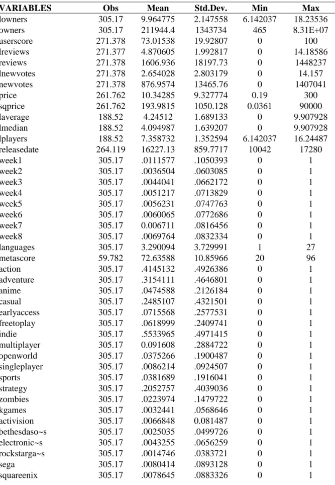
Based on the previously referred event, a treatment and a control group were created depending on whether after September 13, 2016 the URSc of the game had changed. The treatment group is composed by 168,079 observations and the control group by 137,091 observations, making up 55.08% and 44.92% of the total observations, respectively. The average number of owners per game is approximately 212,000, with a maximum above 83 million owners. The average URSc is approximately 73%, which also matches the average metascore (the critics score), being 100% the maximum of both scores. The average change in user scores was a decrease in 0.48 percentage points (pp), which becomes a fall in 1.82pp when we only consider the treatment group, i.e., the games whose score change was different from zero. Lastly, on average, the games were released on June 6, 2014. Complete summary statistics are presented in Table CA.1, alongside the correlation matrix in Table CA.2, in the Complementary Appendices.

IV. Methodology

There is a chronic endogeneity problem when measuring the pure effect of reviews on sales caused by the inherent quality of goods which are reviewed in a certain way. For example, when one decides to go watch a movie which is highly reviewed, does he or she select that specific movie based solely on the rating or because it stars a very famous cast, which could justify the high rating? Thus, in most situations, it is hard to know whether the purchase was motivated simply by the review or by some (un)observable characteristic of the good.

(9)

8 However, on September 13, 2016, the algorithm that Steam uses to compute the URSc was modified. According to information divulged by the organization, it was detected that some games had a disproportional amount of positive or negative reviews coming from users who had been given keys to the games they wrote reviews about, comparing to owners who had paid to acquire the game. As a result, from that day on, Steam no longer used those reviews to calculate the URSc. Such decision lead to abrupt changes in the games’ URSc. This episode enables a quasi-experimental design, as it randomly divided the games into two groups: those whose URSc was altered and those who were not affected. The former can be seen as the treatment group, while the latter will be the control group.

Performing a difference-in-differences analysis between comparable games in the treatment and in the control group enables conclusions to be drawn on the causal effect that the URSc has on the decision to buy a game. Propensity score matching enables the creation of these comparable subgroups, like it is discussed in Stuart et al (2014).

Following the process described in Villa (2012), in a first stage, the identification model has to be defined. The outcome variable is the logarithm of the number of owners, the variable of interest is the URSc and a range of control variables follows:

𝑙𝑜𝑔𝑜𝑤𝑛𝑒𝑟𝑠_𝑖;𝑡 = 𝛽₀+ 𝛽₁𝑈𝑅𝑆𝑐_𝑖;𝑡+ 𝛽₂𝑙𝑜𝑔𝑟𝑒𝑣𝑖𝑒𝑤𝑠_𝑖;𝑡+ 𝛽₃𝑙𝑜𝑔𝑛𝑒𝑤𝑟𝑒𝑣𝑖𝑒𝑤𝑠_𝑖;𝑡 + 𝛽4𝑙𝑜𝑔𝑝𝑟𝑖𝑐𝑒𝑖;𝑡+ 𝛽5𝑙𝑜𝑔𝑠𝑞𝑢𝑎𝑟𝑒𝑑𝑝𝑟𝑖𝑐𝑒𝑖;𝑡+ 𝛽6𝑙𝑜𝑔𝑎𝑣𝑒𝑟𝑎𝑔𝑒𝑡𝑖𝑚𝑒𝑝𝑙𝑎𝑦𝑒𝑑𝑖;𝑡 + 𝛽₇𝑙𝑜𝑔𝑚𝑒𝑑𝑖𝑎𝑛𝑡𝑖𝑚𝑒𝑝𝑙𝑎𝑦𝑒𝑑_𝑖;𝑡 + 𝛽₈𝑙𝑜𝑔𝑝𝑙𝑎𝑦𝑒𝑟𝑠_𝑖;𝑡+ 𝛽₉𝑟𝑒𝑙𝑒𝑎𝑠𝑒𝑑𝑎𝑡𝑒_𝑖;𝑡 + ∑ 𝛽_𝑗𝑤𝑒𝑒𝑘_{𝑖;𝑡;𝑗} 17 𝑗=10 + 𝛽₁₈𝑙𝑎𝑛𝑔𝑢𝑎𝑔𝑒𝑠_𝑖 + 𝛽₁₉𝑚𝑒𝑡𝑎𝑠𝑐𝑜𝑟𝑒_𝑖 + ∑ 𝛽_𝑙𝑡𝑎𝑔𝑠_𝑖;𝑙 33 𝑙=20 + ∑ 𝛽_𝑚𝑝𝑢𝑏𝑙𝑖𝑠ℎ𝑒𝑟_𝑖;𝑚 44 𝑚=34 + ∑ 𝛽_𝑠𝑑𝑒𝑣𝑒𝑙𝑜𝑝𝑒𝑟_𝑖;𝑠 63 𝑠=45 + 𝜀_𝑖;𝑡 (1)

(10)

9 The variables 𝑙𝑜𝑔𝑟𝑒𝑣𝑖𝑒𝑤𝑠_𝑖;𝑡, 𝑙𝑜𝑔𝑛𝑒𝑤𝑟𝑒𝑣𝑖𝑒𝑤𝑠_𝑖;𝑡, 𝑙𝑜𝑔𝑝𝑟𝑖𝑐𝑒_𝑖;𝑡 and 𝑙𝑜𝑔𝑠𝑞𝑢𝑎𝑟𝑒𝑑𝑝𝑟𝑖𝑐𝑒_𝑖;𝑡 are the logarithm of the total number of user reviews, the reviews that were not dismissed by the change in the URSy and are used to calculate the score after the treatment, the price of the game and the square of the game price, respectively. As for 𝑎𝑣𝑒𝑟𝑎𝑔𝑒𝑡𝑖𝑚𝑒𝑝𝑙𝑎𝑦𝑒𝑑_𝑖;𝑡 and 𝑚𝑒𝑑𝑖𝑎𝑛𝑡𝑖𝑚𝑒𝑝𝑙𝑎𝑦𝑒𝑑_𝑖;𝑡, they represent the average and median time played per owner ever since the game was released, respectively, while 𝑙𝑜𝑔𝑝𝑙𝑎𝑦𝑒𝑟𝑠_𝑖;𝑡 is the logarithm of the number of users who have played the game at least once. To account for time effects, 𝑟𝑒𝑙𝑒𝑎𝑠𝑒𝑑𝑎𝑡𝑒_𝑖 and

𝑤𝑒𝑒𝑘𝑖;𝑡;𝑗 were included. The former states how many days have passed since the game was

released and the latter represents a group of j dummy variables, showing if, at the time, the game had been released between 1 and 8 weeks before, one dummy per week. Lastly, the remaining variables control for time-invariant game-specific characteristics. First, 𝑙𝑎𝑛𝑔𝑢𝑎𝑔𝑒𝑠𝑖

is the number of languages the game supports and 𝑚𝑒𝑡𝑎𝑠𝑐𝑜𝑟𝑒_𝑖 is a critics review score. Then, 𝑡𝑎𝑔𝑠_𝑖;𝑙, 𝑝𝑢𝑏𝑙𝑖𝑠ℎ𝑒𝑟_𝑖;𝑚 and 𝑑𝑒𝑣𝑒𝑙𝑜𝑝𝑒𝑟_𝑖;𝑠 are sets of l, m and s dummy variables, identifying the first six tags of each game, i.e., the six most popular categories to include each game in, and publishers and developers selected based on reputation, respectively.

In a second stage, in order to assure a comparable control group, a Kernel Propensity Score Matching process was used. First, a probit model was run, where the outcome variable is the binary variable that states whether the game is in the control or treatment group, with the identification strategy described above. It estimates the propensity scores of each of the games. Following this step, the games were matched by weighing said propensity scores, using the kernel density function.

Finally, in the third stage, the difference-in-differences regression is estimated. The equation shown on the next page is used, which weighs the outcome variable by the Kernel density function and uses 𝑋_𝑖;𝑘 to represent the kth covariate.

(11)

10 𝑙𝑜𝑔𝑜𝑤𝑛𝑒𝑟𝑠_𝑖∗ 𝑤𝑒𝑖𝑔ℎ𝑡𝑠_𝑖

= 𝜃0+ 𝜃1𝑎𝑓𝑡𝑒𝑟𝑖 + 𝜃2𝑡𝑟𝑒𝑎𝑡𝑚𝑒𝑛𝑡𝑖 + 𝜃3𝑎𝑓𝑡𝑒𝑟𝑖 ∗ 𝑡𝑟𝑒𝑎𝑡𝑚𝑒𝑛𝑡𝑖+ 𝜃𝑘𝑋𝑖;𝑘

+ 𝜀_𝑖

(2)

Naturally, the use of the difference-in-differences method requires that the Common Trends assumption is verified. The aim of the matching process is precisely to ensure that both groups are as similar as possible in observables. Without significant differences between the two, there should be no reason to contest the validity of the Common Trends assumption.

Regarding the requirement of common support to conduct the estimation following the matching, it is ensured as the estimation was only done with the observations which were included in the common support.

V. Results

In this section, the results of each of the three stages described in the previous section will be discussed: beginning with the probit, followed by the kernel propensity score matching and, finally, the difference-in-differences to get the average treatment effect (ATE).

The first stage is the probit estimation of the propensity score. The probability of being in the treatment group is positively correlated with factors such as low URSc or metascore and is also higher for more recent games. The complete results are shown in Table CA.3, in the Complementary Appendices.

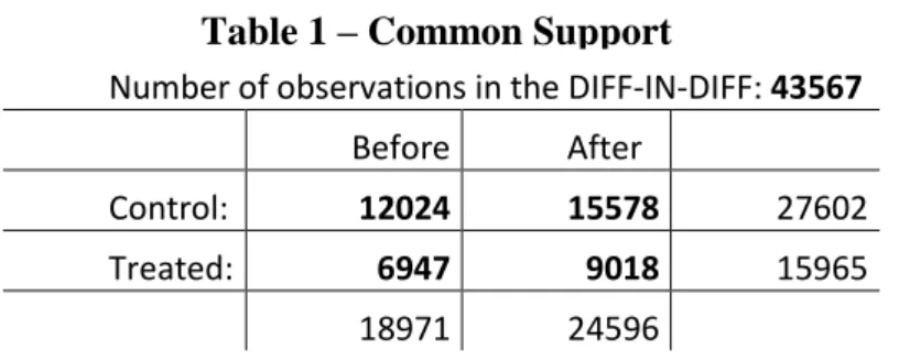
After having estimated the propensity scores, the kernel propensity score matching was performed. The common support comprehends 43,567 observations, which are distributed among the treatment and control groups and before and after the treatment event as Table 1 shows, in the next page.

(12)

11 The benefits of the matching process can be seen at this stage. Upon closer inspection of the distribution of the variables from observations in the treatment and control groups in the baseline time period, significant differences can be identified. However, when only the common support is compared, the differences are in most cases eliminated since these observations are selected on these same observables. There are still some differences but such is the handicap of not having a truly random experiment.

The following graphs provide examples of the outcome of the matching on three selected variables. The pairs of graphs on the right side show the distributions in the common support, while on the left the whole sample is displayed. When the binary variable 𝑡𝑟𝑒𝑎𝑡𝑚𝑒𝑛𝑡_𝑖 takes the value of 1, it means that it is in the treatment group, i.e., the game’s URSc changed.

The logarithm of the owners shows a remarkable improvement in terms of the similarity of the distribution between both groups, in the baseline period. Moreover the concentration that can be seen in Graph 1 on the left tail has disappeared.

Number of observations in the DIFF-IN-DIFF: 43567 Before After

Control: 12024 15578 27602

Treated: 6947 9018 15965

18971 24596 Table 1 – Common Support

0 .1 .2 .3 5 10 15 20 5 10 15 20 0 1 D e n si ty Log(Owners)

treatment=1 means it belongs to the treatment group.

Log(Owners) by Treatment Groups

0 .1 .2 .3 5 10 15 20 5 10 15 20 0 1 D e n si ty Log(Owners)

Log(Owners) by Treatment Groups in the Common Support

(13)

12

Regarding the URSc, in the common support, there are still some differences, mainly in the number of very highly rated games. Nevertheless, the control group no longer has a cluster of games with around 100% user score and they resemble each other more, as intended.

The pattern repeats itself once again when it comes to the logarithm of the number of reviews. The distributions are not exactly equal but the disparity in terms of the left tail vastly decreases and they are both skewed to the left.

Ultimately, the purpose of the propensity score matching is achieved and the treatment and control groups are as similar as possible on observables in the baseline period. Given the similarities between the two groups, it can be assumed that both have common trends. The

0 .0 5 0 50 100 0 50 100 0 1 D e n si ty User Score

User Score by Treatment Groups

0 .1 .2 .3 0 5 10 15 0 5 10 15 0 1 D e n si ty Log(Reviews)

Log(Reviews) by Treatment Groups

0 .0 2 .0 4 .0 6 0 50 100 0 50 100 0 1 D e n si ty User Score

User Score by Treatment Groups in the Common Support

0 .1 .2 .3 0 5 10 15 0 5 10 15 0 1 D e n si ty Log(Reviews)

Log(Reviews) by Treatment Groups in the Common Support

Graph 3 Graph 4

(14)

13 starting point is essentially the same and even the variables in which some difference persists do not raise any plausible reason for the Common Trends assumption not to hold.

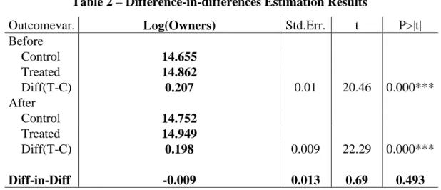
Lastly, the difference-in-differences is conducted and the average treatment effect is calculated. The ATE is computed as the coefficient of the interaction variable, composed by the two dummies that identify the treatment group and the time period after the treatment. The complete results can be seen in column (1) Main Regression of Table A.1, in section IX. Appendices. However, for ease of reference and to focus on the matter, please refer to Table

2, which has the relevant information and also p-values for easier interpretation. In both tables,

the ATE is presented in the row Diff-in-Diff.

According to the estimation, the treatment effect is negative. Given that the treatment caused, on average, a fall of the URSc of 1.8pp, it can be said that the number of owners of a game is expected to decrease by approximately 1% per each 1.8pp decrease in its user review score, on average, ceteris paribus.

Outcomevar. Log(Owners) Std.Err. t P>|t|

Before Control 14.655 Treated 14.862 Diff(T-C) 0.207 0.01 20.46 0.000*** After Control 14.752 Treated 14.949 Diff(T-C) 0.198 0.009 22.29 0.000*** Diff-in-Diff -0.009 0.013 0.69 0.493 R-square: 0.85

* Means and Standard Errors are estimated by linear regression **Robust Std. Errors

**Inference: *** p<0.01; ** p<0.05; * p<0.1

(15)

14 Nevertheless, the effect is not statistically significant as the p-value is 49%, far above the commonly used 5% significance-level. Therefore, the data does not provide any evidence that the user reviews have a causal impact on a game’s owners. Moreover, a poor specification is not to blame, as the R-square is 85%. The result may seem odd but there are some possible explanations:

Hypothesis 1: Due to possible user score manipulation by companies, consumers didn’t care about the score in the first place and did not react to the treatment.

Publishers and developers can offer keys to games, which enables people who did not buy them to write reviews on them. This can influence the user review score and was one of the motives Steam reworked the user review system. As can be read on their website:

“[…] the review score has also become a point of fixation for many developers, to the point where some developers are willing to employ deceptive tactics to generate a more positive review score.

The majority of review score manipulation we're seeing by developers is through the process of giving out Steam keys to their game, which are then used to generate positive reviews. Some developers organize their own system using Steam keys on alternate accounts. Some organizations even offer paid services to write positive reviews.”

(http://store.steampowered.com/news/24155/, written on September 12, 2016) The statement evidences a major distinction between the video game industry and other industries. As was already mentioned, Anderson and Magruder (2012) shows a causal relationship between user restaurant ratings and reservation rates. Furthermore, they also showed that despite having incentives to tamper with the scores, restaurant owners did not do it. Evidently, the same cannot be said of game developers, strengthening the argument to treat the video game sector and possibly the whole digital product market in a different fashion.

Therefore, since gamers could be aware of these practices, they might have become suspicious of the URSc and no longer be influenced by it, when making their purchase decisions.

(16)

15 Hypothesis 2: Users have certain opinions regarding the games, which are not sensitive to changes in the URSc, since all other aspects of the game remain unchanged.

An alternative explanation to the estimated statistically insignificantly different from zero impact of user reviews on the number of a video game’s owners is the characteristic inertia of people’s beliefs. Already subject of academic research, on numerous occasions, people do not update their beliefs, even when given new information. See, for example, Nassar et al (2010).

Potential buyers create an opinion about a game from the moment they become aware of its existence. They base it on multiple elements, some of which were extensively included in the control variables, such as the developer, publisher and genre, but also a friend’s recommendation or the quality of the trailers, screenshots and marketing strategy, in general. It is plausible that once an opinion is formed, it will hardly be modified. Hence, if someone set his or her mind on buying the game, he or she won’t change their decision due to a relatively small average change of the user review score of 1.8 points out of possible 100.

VI. Robustness

The purpose of this section is to modify some elements of the estimation, in order to assess how sensitive the conclusions reached are. Specifically, three new specification strategies will be presented: two of them where the threshold for the treatment variable is made increasingly stricter and the third will change the timespan of the analysis.

In the first case, a game only belongs to the treatment group if the URSc varies by more than 2pp, in absolute value. Remember that, in the main regression, only those whose score did not change are considered part of the control group. This new setting leads to an average change in the treatment group of the URSc of approximately 3.8pp. It also decreases the common support to 31,665 observations, since the treatment group has shrunk and new propensity scores have to be calculated, which affects the matching. The complete results of the

(17)

difference-in-16 differences are shown in column (2) Treatment -2;2 of Table A.1, in section IX. Appendices. Nevertheless, for similar reasons to the ones presented in V. Results, please refer to Table 3.

The results are akin to the ones presented in Table 2. A slightly more negative ATE but the p-value now reaches 61.7%, maintaining the statistical insignificance at a 5% significance-level, and the R-square falls 2pp to 83%. Thus, it seems that more has to be done to try and change the results.

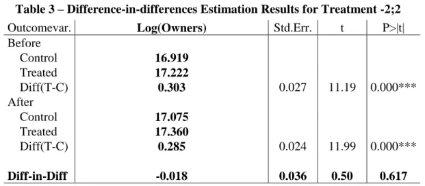
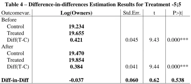
In the second attempt, the treatment variable takes the value of 1 only for games whose URSc varied by more than 5pp, in absolute terms. The average change in the treatment group becomes -6.5pp and the common support shrinks even more, to 17,327 observations. The complete results of the estimation are in column (3) of Table A.1, in section IX. Appendices, but please refer to Table 4, which is on the next page.

Although the ATE now is approximately -4%, once again, the ATE is statistically insignificant at a 5% significance-level, as the p-value is 53.8%, and the R-square falls to 77%. Therefore, it seems that conclusions are not affected by the threshold that defines the treatment and control groups, nor the magnitude of the average URSc change in the treatment.

**Inference: *** p<0.01; ** p<0.05; * p<0.1

(18)

17 For the final robustness test, the time period used to compute the ATE was shortened, while returning to the original definition of the treatment variable. The goal was to check whether focusing on more immediate effects would translate into different results. Thus, only data from one week before and after September 13, 2016 was used. Consequently, the number of observations in the common support becomes 21,824. The results of the estimation are in column (4) of Table A.1, in section IX. Appendices, but please refer to Table 5.

**Inference: *** p<0.01; ** p<0.05; * p<0.1

Table 4 – Difference-in-differences Estimation Results for Treatment -5;5

(19)

18 The results are very similar to the ones of the main regression. The ATE is approximately -1%, while remaining statistically insignificant at the 5% significance-level due to a p-value of 51.9%, and the R-square is the same, at 85%. In conclusion, the results are not affected by changes in the chosen time period.

VII. Policy Implications

The conclusions of this work project are of great importance. No causal relationship between the changes on the number of a game’s owners and the changes on their online user review scores was found. This shows how different markets need to be approached differently. Although the reach of online word-of-mouth has been verified in many industries, it seems that in certain cases it is not so influential.

One possible avenue for video game publishers and developers to increase sales is to invest on their brand power. Perhaps their goal should be to construct a solid fandom, i.e., a group of fans. These will most likely buy their games, regardless of factors such as other users’ opinions, due to their personal relationship with the brand. Consequently, the initial contact with new customers and their initial opinions of the games must be carefully looked into. For example, greater relevance could be given to other sorts of more personal online WOM, as sponsored video game blog posts or known Youtubers’ videos. The multitude of WOM that can be created online and its different effects should be the subject of further research.

In conclusion, video game publishers and developers should disregard marketing strategies that aim to manipulate the user review systems. Besides not being able to find any consequential benefit, to try to deceive customers can have harmful effects in the long run. It might get them high sales in early stages but gamers will eventually lose their trust in the companies behind the games. A recent and famous example in the gaming industry is the game No Man’s Sky, which had a brilliant pre-release marketing campaign and generated very high

(20)

19 expectations, due to its ground-breaking procedurally generated open universe, having over 18 quintillion (1.8x1019) planets embedded in the game’s code, instead of already being written and stored in the game’s files or servers. However, it failed to deliver, as it was plagued by crashes and bugs and the possibilities were not as immense as initially marketed. As a result, a lot of refund requests were made and the creators lost most of the credibility and good-faith they had gained. Another example of the prejudicial effects of lying to the customers, from a different industry, is the September 2015 Volkswagen emission scandal, which lead the German group to lose its leader status in some key markets around the world, facing nowadays very strong competition from Toyota and Renault-Nissan in the global market.

VIII. References

Anderson, Michael, and Magruder, Jeremy. 2012. “Learning from the Crowd: Regression

Discontinuity Estimates of the Effects of an Online Review Database”. The Economic Journal, 122(563): 957-989.

Dellarocas, Chrysanthos, et al.. 2007. “Exploring the value of online product reviews in

forecasting sales: The case of motion pictures”. Journal of Interactive marketing, 21(4): 23–45. Dellarocas, Chrysanthos, et al.. 2010. “Are Consumers More Likely to Contribute Online

Reviews for Hit or Niche Products?”. Journal of Management Information Systems, 27(2): 127– 157.

Entertainment Software Association. 2017. “2017 Essential Facts About the Computer and Video Game Industry”.

Godes, David, and Mayzlin, Dina. 2004. “Using Online Conversations to Study

Word-of-Mouth Communication.” Marketing Science, 23(4): 545–560.

(21)

20 Katz, Elihu, and Lazarsfeld, Paul F.. 1955. “Personal influence: the part played by people in

the flow of mass communications.” Free Press, Glencoe, IL.

Liu, Yong. 2006. “Word of Mouth for Movies: Its Dynamics and Impact on Box Office

Revenue.”. Journal of Marketing, 70(3): 74–89.

McDonald, Emma. 2017. “The Global Games Market Will Reach $108.9 Billion in 2017 With

Mobile Taking 42%”. NewZoo, April 20.

https://newzoo.com/insights/articles/the-global-games-market-will-reach-108-9-billion-in-2017-with-mobile-taking-42/.

Nassar, Mathew R. et al.. 2010. “An Approximately Bayesian Delta-Rule Model Explains the

Dynamics of Belief Updating in a Changing Environment”. Journal of Neuroscience, 30(37): 12366–12378.

Stiglitz, Joseph E.. 1989. “Chapter 13 Imperfect information in the product market”. In

Handbook of Industrial Organization: Volume 1, ed. Richard Schmalensee and Robert D. Willig, 769–847. North Holland: Elsevier B.V..

Stuart, Elizabeth A. et al.. 2014. “Using propensity scores in difference-in-differences models

to estimate the effects of a policy change”. Health Services and Outcomes Research Methodology, 14(4): 166–182.

Takahashi, Dean. 2016. “PwC: Game industry to grow nearly 5% annually through 2020”.

Venture Beat, June 8.

https://venturebeat.com/2016/06/08/the-u-s-and-global-game-industries-will-grow-a-healthy-amount-by-2020-pwc-forecasts/.

Villa, Juan M.. 2012. “Simplifying the estimation of difference in differences treatment effects

(22)

21 IX. Appendices

Table A.1 – Difference-in-Differences Estimation Results

(1) (2) (3) (4)

VARIABLES Main Regression Treatment -2;2 Treatment -5;5 2 Weeks

after 0.0964*** 0.156*** 0.236*** 0.0429 (0.0313) (0.0346) (0.0539) (0.0442) treatment 0.207*** 0.210*** (0.0101) (0.0137) treatment22 0.303*** (0.0271) treatment55 0.421*** (0.0447) Diff-in-Diff -0.00905 -0.0178 -0.0368 -0.0121 (0.0132) (0.0355) (0.0598) (0.0185) userscore -0.00881*** -0.00975*** -0.00771*** -0.00907*** (0.000285) (0.000338) (0.000467) (0.000403) lreviews 0.758*** 0.791*** 0.810*** 0.759*** (0.00498) (0.00570) (0.00883) (0.00701) lnewvotes -0.00983** -0.0184*** -0.0322*** -0.00459 (0.00408) (0.00483) (0.00839) (0.00577) price -0.0211*** -0.0220*** -0.0286*** -0.0221*** (0.000891) (0.000915) (0.00142) (0.00126) sqprice 0.000228*** 0.000224*** 0.000258*** 0.000238***

(1.51e-05) (1.50e-05) (2.43e-05) (2.13e-05)

laverage -0.0202*** -0.0596*** -0.111*** -0.0268*** (0.00710) (0.00834) (0.0130) (0.0102) lmedian 0.00487 0.0499*** 0.0977*** 0.00637 (0.00662) (0.00782) (0.0121) (0.00944) lplayers 0.137*** 0.171*** 0.268*** 0.137*** (0.00498) (0.00586) (0.00856) (0.00707) releasedate -0.000562*** -0.000736*** -0.000929*** -0.000562***

(4.71e-06) (6.17e-06) (1.20e-05) (6.68e-06)

week1 -1.104*** -0.803*** -0.794*** -0.737*** (0.0649) (0.0927) (0.0881) (0.0896) week2 -1.154*** -0.968*** -1.000*** -1.228*** (0.0536) (0.0515) (0.0595) (0.0702) week3 -1.113*** -0.991*** -1.058*** -1.256*** (0.0498) (0.0506) (0.0542) (0.0561) week4 -1.065*** -0.960*** -0.912*** -0.956*** (0.0476) (0.0476) (0.0521) (0.0675) week5 -1.008*** -0.902*** -0.879*** -0.850*** (0.0502) (0.0585) (0.0682) (0.0976) week6 -0.895*** -0.791*** -0.875*** -0.959*** (0.0575) (0.0881) (0.129) (0.0791) week7 -0.807*** -0.587*** -0.598*** -0.915*** (0.0536) (0.0678) (0.0719) (0.0629) week8 -0.871*** -0.539*** -0.485*** -0.609***

(23)

22 (0.0442) (0.0449) (0.0595) (0.0519) languages -0.000872 -0.00100 -0.000741 -0.00100 (0.000818) (0.000887) (0.00155) (0.00116) metascore 0.0109*** 0.0129*** 0.0127*** 0.0114*** (0.000403) (0.000455) (0.000618) (0.000572) Action 0.00132 -0.0111 -0.0217** 0.00117 (0.00664) (0.00764) (0.0107) (0.00943) Adventure 0.0139* 0.0625*** 0.0715*** 0.0148 (0.00735) (0.00834) (0.0111) (0.0104) Anime -0.267*** -0.161*** -0.138*** -0.279*** (0.0136) (0.0144) (0.0182) (0.0190) Casual 0.0377*** 0.0572*** 0.0504** 0.0359** (0.0112) (0.0121) (0.0209) (0.0160) EarlyAccess 0 0 0 0 (0) (0) (0) (0) FreetoPlay 0 0 0 0 (0) (0) (0) (0) Indie 0.0722*** 0.115*** 0.117*** 0.0580*** (0.00761) (0.00823) (0.0115) (0.0108) Multiplayer -0.0705*** -0.100*** -0.152*** -0.0697*** (0.00876) (0.0104) (0.0146) (0.0123) OpenWorld -0.195*** -0.0871*** 0 -0.191*** (0.0123) (0.0153) (0) (0.0174) Single-player 0 0 0 0 (0) (0) (0) (0) Sports -0.117*** 0 0 -0.116*** (0.0183) (0) (0) (0.0258) Strategy 0.151*** 0.167*** 0.251*** 0.157*** (0.00851) (0.00987) (0.0139) (0.0120) Zombies -0.185*** -0.211*** -0.268*** -0.187*** (0.0174) (0.0180) (0.0237) (0.0244) 2KGames 0.0679** -0.367*** 0 0.0618 (0.0337) (0.0473) (0) (0.0479) Activision -0.353*** 0 0 -0.340*** (0.0206) (0) (0) (0.0310) BethesdaSoftworks 0.115*** 0 0 0.107** (0.0353) (0) (0) (0.0502) ElectronicArts -0.175*** 0 0 -0.153*** (0.0300) (0) (0) (0.0432) RockstarGames 0.00818 0 0 0.0293 (0.0287) (0) (0) (0.0400) SEGA 0.381*** 0 0 0.383*** (0.0235) (0) (0) (0.0335) SquareEnix 0.418*** 0.358*** 0.341*** 0.405*** (0.0220) (0.0294) (0.0373) (0.0310) THQNordic 0.340*** 0.528*** 0 0.327*** (0.0195) (0.0225) (0) (0.0281) TelltaleGames 1.135*** 1.175*** 0 1.083*** (0.116) (0.0953) (0) (0.161) Valve -0.106** 0 0 -0.144*

(24)

23 (0.0507) (0) (0) (0.0737) WarnerBros. 0.247*** 0.0539 0 0.236*** (0.0324) (0.0348) (0) (0.0458) BioWare 0.305*** 0 0 0.296*** (0.0626) (0) (0) (0.0894) Capcom -0.126*** -0.316*** -0.657*** -0.124*** (0.0223) (0.0254) (0.0332) (0.0313) CDPROJEKTRED 0 0 0 0 (0) (0) (0) (0) DICE 0 0 0 0 (0) (0) (0) (0) FiraxisGames 0.715*** 0 0 0.720*** (0.0558) (0) (0) (0.0792) GearboxSoftware -0.111*** 0.0297 0 -0.139*** (0.0306) (0.0358) (0) (0.0418) IOInteractive -0.338*** 0 0 -0.324*** (0.0345) (0) (0) (0.0494) LucasArts 0.697*** 0 0 0.688*** (0.0341) (0) (0) (0.0471) MumboJumbo 0 0 0 0 (0) (0) (0) (0) ObsidianEntertainment -0.0315 0 0 -0.0256 (0.0321) (0) (0) (0.0475) RelicEntertainment 0.512*** 0 0 0.499*** (0.0734) (0) (0) (0.104) SquareEnixDEV -0.0635*** 0 0 -0.0541*** (0.0137) (0) (0) (0.0192) TelltaleGamesDEV -0.672*** -0.898*** 0 -0.633*** (0.107) (0.0876) (0) (0.148) TheCreativeAssembly -0.288** 0 0 -0.304* (0.124) (0) (0) (0.175) Treyarch 0.490*** 0 0 0.487*** (0.0720) (0) (0) (0.102) TripwireInteractive 0 0 0 0 (0) (0) (0) (0) UbisoftDEV 0 0 0 0 (0) (0) (0) (0) ValveDEV 0 0 0 0 (0) (0) (0) (0) Constant 14.66*** 16.92*** 19.23*** 14.67*** (0.0808) (0.101) (0.191) (0.114) Observations 43,567 31,665 17,327 21,824 R-squared 0.852 0.825 0.773 0.852

Robust standard errors in parentheses *** p<0.01, ** p<0.05, * p<0.1

(25)

24 Complementary Appendices

Table CA.1 – Descriptive Statistics

VARIABLES Obs Mean Std.Dev. Min Max

lowners 305.17 9.964775 2.147558 6.142037 18.23536 owners 305.17 211944.4 1343734 465 8.31E+07 userscore 271.378 73.01538 19.92807 0 100 lreviews 271.377 4.870605 1.992817 0 14.18586 reviews 271.378 1606.936 18197.73 0 1448237 lnewvotes 271.378 2.654028 2.803179 0 14.157 newvotes 271.378 876.9574 13465.76 0 1407041 price 261.762 10.34285 9.327774 0.19 300 sqprice 261.762 193.9815 1050.128 0.0361 90000 laverage 188.52 4.24512 1.689133 0 9.907928 lmedian 188.52 4.094987 1.639207 0 9.907928 lplayers 188.52 7.358732 1.352594 6.142037 16.24487 releasedate 264.119 16227.13 859.7717 10042 17280 week1 305.17 .0111577 .1050393 0 1 week2 305.17 .0036504 .0603085 0 1 week3 305.17 .0044041 .0662172 0 1 week4 305.17 .0051217 .0713829 0 1 week5 305.17 .0056231 .0747763 0 1 week6 305.17 .0060065 .0772686 0 1 week7 305.17 0.006711 .0816456 0 1 week8 305.17 .0069764 .0832334 0 1 languages 305.17 3.290094 3.729991 1 27 metascore 59.782 72.63588 10.85966 20 96 action 305.17 .4145132 .4926386 0 1 adventure 305.17 .3154111 .4646801 0 1 anime 305.17 .0474588 .2126184 0 1 casual 305.17 .2485107 .4321501 0 1 earlyaccess 305.17 .0715568 .2577531 0 1 freetoplay 305.17 .0618999 .2409741 0 1 indie 305.17 .5533965 .4971415 0 1 multiplayer 305.17 0.091608 .2884722 0 1 openworld 305.17 .0375266 .1900487 0 1 singleplayer 305.17 .0086214 .0924507 0 1 sports 305.17 .0381689 .1916041 0 1 strategy 305.17 .2052757 .4039036 0 1 zombies 305.17 .0223974 .1479722 0 1 kgames 305.17 .0032441 .0568646 0 1 activision 305.17 .0066848 0.081487 0 1 bethesdaso~s 305.17 .0025035 .0499726 0 1 electronic~s 305.17 .0043255 .0656259 0 1 rockstarga~s 305.17 .0014746 .0383721 0 1 sega 305.17 .0080414 .0893128 0 1 squareenix 305.17 .0078645 .0883326 0 1

(26)

25 thqnordic 305.17 .0088148 .0934724 0 1 telltalega~s 305.17 .0051119 .0713147 0 1 valve 305.17 .0031458 .0559991 0 1 warnerbros 305.17 .0029492 .0542263 0 1 bioware 305.17 .0005898 .0242794 0 1 capcom 305.17 .0020251 .0449556 0 1 cdprojektred 305.17 .0002949 .0171707 0 1 dice 305.17 .0002949 .0171707 0 1 firaxisgames 305.17 .0011797 .0343261 0 1 gearboxsof~e 305.17 .0008848 .0297317 0 1 iointeract~e 305.17 .0007864 .0280327 0 1 lucasarts 305.17 0.001278 0.035726 0 1 mumbojumbo 305.17 .0034374 .0585288 0 1 obsidianen~t 305.17 .0006881 .0262235 0 1 relicenter~t 305.17 .0007766 .0278571 0 1 squareenix~v 305.17 .0037356 .0863557 0 2 telltalega~v 305.17 .0052102 .0719936 0 1 thecreativ~y 305.17 .0002949 .0171707 0 1 treyarch 305.17 .0007864 .0280327 0 1 tripwirein~e 305.17 .0003932 0.019826 0 1 ubisoftdev 305.17 .0043255 .0656259 0 1 valvedev 305.17 .0027526 .0523927 0 1 treatment 305.17 .4492283 .4974164 0 1 diffscore 285.711 -.479565 6.370476 -98 70 after 305.17 .6109939 .4875255 0 1

(27)

26 Table CA.2 – Correlation Matrix

lo w ner s us er sc ~e lrev iew s ln ew vo ~s pr ic e sq pr ic e la ver ag e lm ed ia n lp la yer s rel ea s~e la ng ua ~s m eta sc ~e tr ea tm ~t af ter lo w ner s 1 us er sc o re 0. 19 8 1 lrev iew s 0. 81 0 0. 29 6 1 ln ew vo tes 0. 21 6 0. 07 4 0. 25 8 1 pr ic e 0. 10 7 0. 00 2 0. 31 5 0. 07 7 1 sq pr ic e 0. 08 8 -0 .0 12 0. 23 6 0. 05 7 0. 91 0 1 la ver ag e 0. 24 5 0. 16 0 0. 32 4 0. 08 4 0. 27 7 0. 19 8 1 lm ed ia n -0 .0 29 0. 05 0 0. 01 3 0. 00 7 0. 16 0 0. 11 3 0. 87 7 1 lp la yer s 0. 68 9 0. 29 8 0. 83 6 0. 20 5 0. 40 1 0. 31 6 0. 44 0 0. 08 6 1 rel ea sed ate -0 .4 38 -0 .0 09 -0 .0 41 -0 .0 15 0. 28 6 0. 21 7 0. 02 4 0. 07 9 -0 .0 08 1 la ng ua ges 0. 22 6 0. 05 3 0. 36 3 0. 09 3 0. 25 4 0. 17 6 0. 18 0 0. 06 6 0. 37 7 0. 13 6 1 m eta sc o re 0. 38 2 0. 55 8 0. 34 8 0. 09 1 0. 12 7 0. 10 7 0. 20 0 0. 04 4 0. 39 6 -0 .1 97 0. 05 9 1 tr ea tm en t -0 .2 25 -0 .2 22 -0 .2 78 -0 .0 76 -0 .0 25 -0 .0 22 -0 .1 17 -0 .0 23 -0 .2 10 0. 15 6 -0 .0 59 -0 .2 31 1 af ter 0. 01 0 -0 .0 02 0. 00 5 0. 94 1 0. 00 3 0. 00 1 0. 00 5 0. 00 6 -0 .0 05 0. 00 4 0. 00 3 0. 00 1 0. 00 1 1

(28)

27 Table CA.3 – Probit Regression to calculate Propensity Scores

Probit regression Number of obs = 19249

LR chi2(52) = 3311.57

Prob > chi2 = 0.0000

Loglikelihood = -10932.959 _{PseudoR2=0.1315}

Treatment Coef. Std. Err. z P>|z|

userscore -.0150199 .0008704 -17.26 0.000*** lreviews -.3138634 .0130525 -24.05 0.000*** price .0138958 .0026743 5.20 0.000*** sqprice -.0001655 .0000419 -3.95 0.000*** laverage -.0866508 .0242414 -3.57 0.000*** lmedian .0505344 .0228138 2.22 0.027** lplayers .1715067 .0161413 10.63 0.000*** releasedate .0001379 .0000133 10.35 0.000*** week1 .34651 .2073262 1.67 0.095* week2 .5918188 .1760343 3.36 0.001*** week3 .1363872 .1861791 0.73 0.464 week4 -.7222578 .2330219 -3.10 0.002*** week5 .1631291 .2105297 0.77 0.438 week6 .9882958 .2523809 3.92 0.000*** week7 .1990192 .2298656 0.87 0.387 week8 .482154 .2076047 2.32 0.020** languages .0015304 .0028834 0.53 0.596 metascore -.0078557 .0012834 -6.12 0.000*** action .2361013 .0226317 10.43 0.000*** adventure .1437587 .0251786 5.71 0.000*** anime -.0314537 .0647408 -0.49 0.627 casual .0689664 .0372939 1.85 0.064* indie .2998386 .025792 11.63 0.000*** multiplayer -.054341 .030623 -1.77 0.076* openworld .0212448 .0470803 0.45 0.652 sports -.0190094 .0595336 -0.32 0.749 strategy .0868336 .0274166 3.17 0.002*** zombies -.1471901 .0672837 -2.19 0.029** kgames .1227787 .118476 1.04 0.300 activision -.1060774 .1100118 -0.96 0.335 bethesdaso~s .270947 .0953302 2.84 0.004*** electronic~s -.9040765 .124461 -7.26 0.000*** rockstarga~s -.1583564 .1555282 -1.02 0.309 sega .4014912 .0962517 4.17 0.000*** squareenix -.1881256 .0714217 -2.63 0.008*** thqnordic -.1444694 .0545663 -2.65 0.008*** telltalega~s .1529674 .3029959 0.50 0.614 valve -5.688059 .1268442 -44.84 0.000*** warnerbros -.0137148 .1049003 -0.13 0.896 bioware 1.158276 .2161746 5.36 0.000*** capcom -.0066959 .1023783 -0.07 0.948

(29)

28 firaxisgames .3762701 .1524423 2.47 0.014** gearboxsof~e 1.066681 .2467913 4.32 0.000*** iointeract~e 1.481941 .1675785 8.84 0.000*** lucasarts -.2463514 .2057303 -1.20 0.231 obsidianen~t .1218065 .2017681 0.60 0.546 relicenter~t .4551792 .1884168 2.42 0.016** squareenix~v -.0908546 .0889025 -1.02 0.307 telltalega~v .6852268 .3001559 2.28 0.022** thecreativ~y .5945643 .251777 2.36 0.018** treyarch .8556419 .2416324 3.54 0.000*** _cons -.2661982 .2259048 -1.18 0.239

(30)

29 CA.4 – Stata Codes

*KERNEL PROPENSITY SCORE DiD

use "E:\Documentos\NOVA\Mestrado\Work Project\FINAL MERGED DATA September.dta"

set more off

global tags action adventure anime casual earlyaccess freetoplay indie multiplayer openworld singleplayer sports strategy zombies

global publisher kgames activision bethesdasoftworks electronicarts rockstargames sega squareenix thqnordic telltalegames valve warnerbros

global developer bioware capcom cdprojektred dice firaxisgames gearboxsoftware

iointeractive lucasarts mumbojumbo obsidianentertainment relicentertainment squareenixdev telltalegamesdev thecreativeassembly treyarch tripwireinteractive ubisoftdev valvedev global week week1 week2 week3 week4 week5 week6 week7 week8

xtset app_id date, format(%tdDD/NN/CCYY) set more off

diff lowners if support==1, t(treatment) p(after) cov( userscore lreviews lnewvotes price sqprice laverage lmedian lplayers releasedate $week languages metascore $tags $publisher $developer ) robust report

diff lowners , t(treatment) p(after) cov( userscore lreviews lnewvotes price sqprice laverage lmedian lplayers releasedate $week languages metascore $tags $publisher $developer ) kernel id(app_id) robust report

*Exporting

outreg2 using "did.doc", replace ctitle(Main Regression) label outreg2 using "did.doc", append ctitle(Treatment -2;2) label outreg2 using "did.doc", append ctitle(Treatment -5;5) label outreg2 using "did.doc", append ctitle(Week Before&After) label

*Descriptive Statistics

tab treatment

tab support if _merge_treatment==3

sum lowners owners userscore lreviews reviews lnewvotes newvotes price sqprice laverage lmedian lplayers releasedate $week languages metascore $tags $publisher $developer treatment diffscore after if _merge_treatment==3

(31)

30 mean diffscore

mean diffscore if diffscore~=0

gen diffscore22=diffscore*treatment22 mean diffscore22 if diffscore22~=0 gen diffscore55=diffscore*treatment55 mean diffscore55 if diffscore55~=0

correlate lowners userscore lreviews lnewvotes price sqprice laverage lmedian lplayers releasedate languages metascore treatment after

correlate lowners userscore lreviews lnewvotes price sqprice laverage lmedian lplayers releasedate $week languages metascore $tags $publisher $developer treatment after hist lowners, by(treatment)

hist userscore, by(treatment) hist releasedate, by(treatment)

hist lowners if after==0, by(treatment) hist userscore if after==0, by(treatment) hist releasedate if after==0, by(treatment)

hist lowners if after==0 & support==1, by(treatment) hist userscore if after==0 & support==1, by(treatment) hist releasedate if after==0 & support==1, by(treatment)

histogram lowners if after==0, xtitle(Log(Owners)) by(, title(Log(Owners) by Treatment Groups) note(treatment=1 means it belongs to the treatment group.)) by(treatment)

histogram userscore if after==0, xtitle(User Score) by(, title(User Score by Treatment Groups) note(treatment=1 means it belongs to the treatment group.)) by(treatment)

histogram lreviews if after==0, xtitle(Log(Reviews)) by(, title(Log(Reviews) by Treatment Groups) note(treatment=1 means it belongs to the treatment group.)) by(treatment)

histogram releasedate if after==0, xtitle(Release Date) by(, title(Release Date by Treatment Groups) note(treatment=1 means it belongs to the treatment group. Variable is in days since release coded for days since 01/01/1970)) by(treatment)

histogram lowners if after==0 & support==1, xtitle(Log(Owners)) by(, title(Log(Owners) by Treatment Groups in the Common Support) note(treatment=1 means it belongs to the

treatment group.)) by(treatment)

histogram userscore if after==0 & support==1, xtitle(User Score) by(, title(User Score by Treatment Groups in the Common Support) note(treatment=1 means it belongs to the treatment group.)) by(treatment)

(32)

31 histogram lreviews if after==0 & support==1, xtitle(Log(Reviews)) by(, title(Log(Reviews) by Treatment Groups in the Common Support) note(treatment=1 means it belongs to the treatment group.)) by(treatment)

histogram releasedate if after==0 & support==1, xtitle(Release Date) by(, title(Release Date by Treatment Groups in the Common Support) note(treatment=1 means it belongs to the treatment group. Variable is in days since release coded for days since 01/01/1970)) by(treatment)

*New Treatment Assignment

use "E:\Documentos\NOVA\Mestrado\Work Project\FINAL MERGED DATA September.dta"

sort app_id date

gen diffscore=newscore-userscore replace diffscore=0 if date<17058

gen diffscore14=userscore-newscore if date==17058 tab diffscore14

keep if date==17058 gen treatment=1

replace treatment=0 if diffscore14==0 | diffscore14==. gen treatment22=1

gen treatment55=1

merge m:1 app_id using "E:\Documentos\NOVA\Mestrado\Work Project\Treatment and Diffscore.dta", generate(_merge_treatment)

merge m:1 app_id using "E:\Documentos\NOVA\Mestrado\Work Project\Treatment 55.dta", generate(_merge_treatment55)

*Robustness Checks

diff lowners, t(treatment22) p(after) cov( userscore lreviews lnewvotes price sqprice laverage lmedian lplayers releasedate $week languages metascore $tags $publisher $developer ) kernel id(app_id) support robust report

(33)

32 gen support22=_support

diff lowners if support22==1, t(treatment22) p(after) cov( userscore lreviews lnewvotes price sqprice laverage lmedian lplayers releasedate $week languages metascore $tags $publisher $developer ) robust report

set more off

diff lowners, t(treatment55) p(after) cov( userscore lreviews lnewvotes price sqprice laverage lmedian lplayers releasedate $week languages metascore $tags $publisher $developer ) kernel id(app_id) support robust report

gen support55=_support

diff lowners if support55==1, t(treatment55) p(after) cov( userscore lreviews lnewvotes price sqprice laverage lmedian lplayers releasedate $week languages metascore $tags $publisher $developer ) robust report

*xtreg Experimentation

gen pt=treated*after

xtreg lowners after pt average mediantime players price sqprice $tags $publisher $developer $week releasedate languages userscore metascore, robust

xtreg lowners after pt average mediantime players price sqprice $tags $publisher $developer $week releasedate languages userscore metascore, fe robust

gen before1=0

replace before1=1 if date<=17050 gen before2=0

replace before2=1 if date<=17056 & date>17050 gen after1=0

replace after1=1 if date<=17062 & date>17056 gen after2=0

replace after2=1 if date<=17068 & date>17062 gen after3=0

replace after3=1 if date>17068 gen pt1=after1*treated

gen pt2=after2*treated gen pt3=after3*treated

xtreg lowners after pt1 pt2 pt3 average mediantime players price sqprice $tags $publisher $developer $week releasedate languages userscore metascore, fe robust

(34)

33 xtreg lowners after pt pt1 pt2 pt3 average mediantime players price sqprice $tags $publisher $developer $week releasedate languages userscore metascore, fe robust

*Initial Processing

import delimited "E:\Documentos\NOVA\Mestrado\Work Project\FinalData.csv", delimiter(";") drop if dates<1470009600000 drop if dates>1477872000000 gen date=dates/86400000 drop if owners==. drop dates

xtset app_id date, daily

gen MA7owners = (F3.owners + F2.owners + F1.owners + owners + L1.owners + L2.owners + L3.owners) / 7

gen lowners=log(owners) gen sqprice=price^2

gen after=1 if d1970>17056 replace after=0 if after==. gen lplayers=log(players) gen laverage=log(average) gen lmedian=log(mediantime) gen reviews=positive+negative gen lreviews=log(reviews) *September

drop if date<17045 | date>17074

*2weeks

drop if date<17051 | date>17065

*Merge Web & Reviews

use "E:\Documentos\NOVA\Mestrado\Work Project\FINAL DATA.dta", clear

merge m:m app_id datestring using "E:\Documentos\NOVA\Mestrado\Work Project\Data Reviews FINAL.dta", force

(35)

34

*Release Date Variables

gen days= date - releasedate gen weeks=days/7

gen week1=0

replace week1=1 if weeks<=1 gen week2=0

replace week2=1 if weeks<=2 & weeks>1 gen week3=0

replace week8=1 if weeks<=8 & weeks>7

*Data Robustness Check 2016

import delimited "E:\Documentos\NOVA\Mestrado\Work Project\FinalData.csv", delimiter(";")

gen date=dates/86400000 drop dates

gen var10=date

xtset app_id date, format(%tdNN/DD/CCYY) gen yearvariation=F250.owners-owners

gen ownersvariation=yearvariation if var10==16916 gsort - ownersvariation

(36)

35 CA.5 – Python Codes for Web Scraping

import requests

from lxml import html

from lxml.etree import tostring import json import pandas as pd import re import time import os os.chdir(r"E:\Documentos\NOVA\Mestrado\Work Project") db1 = pd.read_stata("Data Reviews FINAL.dta")

db1["db1"] = 1

db2 = pd.read_stata("FINAL DATA.dta") db1["db1"] = 0

mergedata = pd.merge(db1, db2, on = ["app_id", "datestring"], how="right") mergedata.to_stata("MergedData.dta") db3 = pd.read_stata("Preliminary Merge.dta") db3.groupby("app_id")["date"].value_counts().to_csv("test.csv", index=1) Steam DB all_app_ids = [] all_game_names = [] all_app_types = [] n_pages = int(html.fromstring(requests.get("https://steamdb.info/apps/page1/").content).xpath('/html/bod y/div[1]/div[2]/div/h1[1]/text()[2]')[0][1:])

for page in range(1,n_pages+1):

raw_page = requests.get("https://steamdb.info/apps/page"+str(page)+"/") tree = html.fromstring(raw_page.content)

(37)

36 game_name = [x.text for x in tree.xpath("//tr/td[3]/a")]

game_name = list(filter(lambda x: x!="\n", game_name)) app_type = [x.text for x in tree.xpath("//tr/td[3]/i")]

all_app_ids = all_app_ids+app_id

all_game_names = all_game_names+game_name all_app_types = all_app_types+app_type

steamdb = pd.DataFrame(data = [all_app_ids, all_game_names, all_app_types]).T steamdb.columns = ["app_id", "app_name", "app_type"]

steamdb.to_csv("steamdb.csv",index=0)

Steam Spy

from robobrowser import RoboBrowser

browser = RoboBrowser(history=True, parser="lxml") browser.open("http://steamspy.com/login")

form = browser.get_form("login_form")

form["username"] = "CapitaoPortugal" #Põe entre "" o teu username form["password"] = "Recroom00" ##Põe entre "" a tua password browser.submit_form(form)

def get_dataset_boundaries(code): iter_start = re.finditer("\{", code)

indices_start = [m.start(0) for m in iter_start] iter_end = re.finditer("\}", code)

indices_end = [m.end(0) for m in iter_end] return indices_start, indices_end

steamdb = pd.read_csv("IDsnoerrors.csv", encoding="latin", sep=";") #Para carregar a base que tenhas guardado. Remove o #

steamdb.columns = ["app_id", "name"] #for app_id in steamdb["app_id"]:

(38)

37 #for app_id in ['268500']:

for app_id in steamdb["app_id"]: print(app_id) #time.sleep(.2) browser.open("http://steamspy.com/app/"+str(app_id)) tree = html.fromstring(browser.response.content) #tab-sales tab_sales = tree.xpath('//*[@id="tab-sales"]/script/text()')[0].replace("\n","").replace("\r","").replace(" ", "").replace(",,",',"",').replace("\\'","").replace("\\","") tab_sales = re.sub('(?<=\w)"(?=\w)',"",tab_sales) tab_sales = re.sub('(?<=\w)""','"',tab_sales) tab_sales = re.sub('""(?=\w)','"',tab_sales) tab_sales = re.sub('(?<=[<?+!-*=])""','"',tab_sales) tab_sales = re.sub('""(?=[<?+!-*=])','"',tab_sales) tab_sales = re.sub('(?<=\w)"(?=[<?+!-*=])',"",tab_sales) tab_sales = re.sub('(?<=[<?+!-*=])"(?=\w)',"",tab_sales) starts, ends = get_dataset_boundaries(tab_sales)

owners_data = json.loads(tab_sales[starts[0]:ends[0]]) dates = [row[0] for row in owners_data["values"]] owners = [row[1] for row in owners_data["values"]] owners_data = pd.DataFrame(data = [dates, owners]).T owners_data.columns = ["dates", "owners"]

owners_data["app_id"] = app_id

prices_data = json.loads(tab_sales[starts[1]:ends[1]]) dates = [row[0] for row in prices_data["values"]] prices = [row[1] for row in prices_data["values"]]

(39)

38 prices_data.columns = ["dates", "prices"]

prices_data["app_id"] = app_id

merge = pd.merge(owners_data, prices_data, on = ["dates", "app_id"]) #tab-audience tab_audience = tree.xpath('//*[@id="tab-audience"]/script/text()')[0].replace("\n","").replace("\r","").replace(" ", "").replace(",,",',"",').replace(",,",',"",').replace("\\'","").replace("\\","") tab_audience = re.sub('(?<=\w)"(?=\w)',"",tab_audience) tab_audience = re.sub('(?<=\w)""','"',tab_audience) tab_audience = re.sub('(?<=[<?+!-*=])""','"',tab_audience) tab_audience = re.sub('""(?=[<?+!-*=])','"',tab_audience) tab_audience = re.sub('(?<=\w)"(?=[<?+!-*=])',"",tab_audience) tab_audience = re.sub('(?<=[<?+!-*=])"(?=\w)',"",tab_audience) starts, ends = get_dataset_boundaries(tab_audience)

players_data = json.loads(tab_audience[starts[0]:ends[0]]) dates = [row[0] for row in players_data["values"]]

players = [row[1] for row in players_data["values"]] players_data = pd.DataFrame(data = [dates, players]).T players_data.columns = ["dates", "players"]

players_data["app_id"] = app_id

average_data = json.loads(tab_audience[starts[1]:ends[1]].replace(',]',',""]')) dates = [row[0] for row in average_data["values"]]

average = [row[1] for row in average_data["values"]] average_data = pd.DataFrame(data = [dates, average]).T average_data.columns = ["dates", "average"]

average_data["app_id"] = app_id

median_data = json.loads(tab_audience[starts[2]:ends[2]].replace(',]',',""]')) dates = [row[0] for row in median_data["values"]]

median = [row[1] for row in median_data["values"]] median_data = pd.DataFrame(data = [dates, median]).T

(40)

39 median_data.columns = ["dates", "median"]

median_data["app_id"] = app_id

merge2 = pd.merge(merge, players_data, on = ["dates", "app_id"]) merge3 = pd.merge(merge2, average_data, on = ["dates", "app_id"]) merge4 = pd.merge(merge3, median_data, on = ["dates", "app_id"])

def clean(l):

return ", ".join(list(filter(None,[re.sub('[<>, ]',"",x) for x in re.findall('\>.*?\<',l)])))

def clean2(l):

return ", ".join(list(filter(None,[re.sub('[<> ]',"",x) for x in re.findall('\>.*?\<',l)]))).replace(",",", ")

a = tree.xpath('//div[@class="p-r-30"]/p')[0] b = tostring(a).decode("utf-8")

raw_list = [i for i in b.split("<strong>")][1:]

categories_list = [i.split("<")[0].replace(":","") for i in raw_list] try: merge4["developer"] = clean(raw_list[0])

except: pass

try: merge4["publisher"] = clean(raw_list[1]) except: pass

try: merge4["genre"] = clean(raw_list[2]) except: pass

try: merge4["languages"] = clean(raw_list[3]) except: pass

try: merge4["tags"] = clean(raw_list[4]) except: pass

try: merge4["category"] = clean2(raw_list[5]) except: pass

(41)

40 except: pass

try: merge4["metascore"] = clean(raw_list[11]) except: pass

merge_final = pd.concat([merge_final,merge4]) merge_final.to_csv("FinalData.csv", index=0, sep=";")