A Comparative Analysis of
Financing Decisions
in export and non-export sectors: the
case of Spanish non-listed firms
Master Final Work in the modality of Dissertation presented to Universidade Católica Portuguesa to fulfill the requirements for the degree of Msc in Finance
by
Mário Pedro Rodrigues Pinto
Católica Porto Business School June 2019
A Comparative Analysis of
Financing Decisions
in export and non-export sectors: the
case of Spanish non-listed firms
Master Final Work in the modality of Dissertation presented to Universidade Católica Portuguesa to fulfill the requirements for the degree of Msc in Finance
by
Mário Pedro Rodrigues Pinto
under the supervision of
Professor Dr. João Filipe Monteiro Pinto
Católica Porto Business School June 2019
iii
Acknowledgments
Since this work is the culmination of all academic learning that I had, this paragraph is dedicated to those who made this work possible in every aspects.
First of all, I would like to thank my parents, Cristina and Mário, for all the support they gave me during all stages in my life, academically, sportively and personally. Without their support, nothing that I have achieved until now would be possible.
Secondly, I would like to thank my grandmothers, Arminda and Marilda, my grandfathers, Francisco and Soter, and my uncle, Sotero, for having such an important role in my life and have guided me, specially, in the beginning of my life.
Then, I have to give a special word to my girlfriend, Beatriz, for being always by my side during my academic life and help me to pass through the problems that I have faced. Without you, this path would have been much more difficult than it was.
Also, I would like to thank to all my friends for being by my side in the good and bad moments and supporting me when I needed the most.
I would like to thank to my bosses at Millennium BCP, Hélder Oliveira and Manuel Pinho, where I worked from January to May, for giving me some freedom to finish my thesis.
Last but not least, I would like to thank my supervisor Professor Dr. João Filipe Monteiro Pinto for all the availability, wisdom and good advices and Professor Ricardo Ribeiro for all his help regarding the econometric model.
v
Resumo
Esta tese tem como objetivo estudar as diferenças nas decisões de financiamento entre as empresas exportadoras e não-exportadoras não cotadas em Espanha e, também, examinar qual é o impacto da intensidade de exportação no nível de endividamento das mesmas empresas. Para isso, usamos uma amostra composta por 45 147 empresas, durante o período de 2012 a 2017.
Após uma revisão detalhada da literatura, foi feita uma análise usando diferentes determinantes que, de acordo com a literatura existente, têm impacto na estrutura de capital das empresas (e consequentemente nas suas decisões de financiamento): Impostos, Tangibilidade, Rentabilidade, Dimensão da Empresa, Outros Benefícios Fiscais para além da Dívida, Condições da Indústria, Risco de Negócio, Oportunidades de Crescimento, Taxa de Inflação e Intensidade de Exportação.
Os resultados obtidos sugerem que, embora alguns fatores estejam de acordo com a literatura existente, tal como o impacto dos Impostos, da Tangibilidade, da Rentabilidade, das Condições de Indústria, do Risco de Negócio e da Taxa de Inflação; a Dimensão da Empresa e os Outros Benefícios Fiscais para além da Dívida apresentam impactos no nível da dívida diferentes dos esperados. Para além disso, o único fator cujos resultados diferem das empresas exportadoras para as empresas não exportadoras são os Impostos, que apresenta um impacto negativo na alavancagem para empresas exportadoras e positivo para com as não exportadoras. Finalmente, verifica-se que a Intensidade de Exportação tem uma relação positiva com o nível de endividamento.
Palavras-Chave: Decisões de Financiamento, Estrutura de Capital, Exportações, Empresas Espanholas Não Cotadas.
vii
Abstract
The purpose of this thesis is to study the differences in the financing decisions between non-listed Spanish export and non-export firms, as well as to examine what is the impact of export intensity in firm’s leverage. To do so, we use a sample of 45,147 Spanish unlisted firms during the 2012-2017 period.
After a detailed literature review, an analysis was made using different determinants that, according to the extant literature, impact the capital structure (and consequently, the financing decisions): Taxes, Tangibility, Profitability, Firm Size, Non-Debt Tax Shields, Industry Conditions, Business Risk, Growth Opportunities, Inflation Rate and Export Intensity.
The results obtained suggest that while the impact of some factors are in line with the extant literature, namely Taxes, Tangibility, Profitability, Industry Conditions, Business Risk and Inflation Rate; the impact of Firm Size and Non-Debt Tax Shields is different from what we expected. Furthermore, the only factor that affects differently both export and non-export firms is Taxes, which presents a negative correlation with export firms’ leverage and positive with non-export firms’ leverage. Finally, the variable Export Intensity shows a positive relationship with Leverage.
Keywords: Financing Decisions, Capital Structure, Exportations, Spain Unlisted Firms.
ix
Index
Resumo ... v
Abstract ... vii
Index of Graphs ... xi
Index of Tables ...xiii
Appendices Index ... xv
Introduction ... 17
Chapter 1 ... 21
1. General Framework... 21
1.1. Spain’s GDP ... 22
1.2. Spain Terms of Trade ... 23
1.3. Spain Balance of Trade ... 24
1.4. Spain Exportations ... 25
1.5. Spain Inflation Rate ... 26
Chapter 2 ... 27
2. Literature Review ... 27
2.1. Capital Structure Theories ... 27
2.2. Determinants of Capital Structure ... 36
Chapter 3 ... 46
3. Research Questions and Hypothesis ... 46
3.1. Research Questions ... 46
3.2. Research hypotheses ... 46
x
4. Variables, Sample, Descriptive Statistics and Methodology ... 51
4.1. Variables ... 51 4.2. Sample ... 52 4.3. Descriptive Statistics ... 54 4.4. Preliminary Analysis ... 62 4.5. Methodology ... 63 Chapter 5 ... 65
5. Regression results and Deviations from the literature ... 65
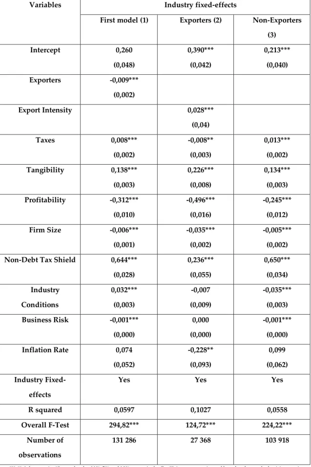
5.1. Regression Results ... 65
5.2. Deviations from the literature ... 70
5.3. Model with Growth Opportunities ... 74
Conclusion ... 76
References ... 78
xi
Index of Graphs
Graph 1 – Spain’s GDP growth rate in the 2012-2017 period. ... 22
Graph 2 – Spain’s Terms of Trade in the 2012-2017 period. ... 23
Graph 3 – Spain’s Balance of Trade in the 2012-2017 period. ... 24
Graph 4 – Spain’s exports in the 2012-2017 period. ... 25
Graph 5 – Spain’s Inflation Rate in the 2012-2017 period. ... 26
Graph 6 – Median leverage by year for All firms ... 58
Graph 7 – Exporters median leverage by year. ... 59
xiii
Index of Tables
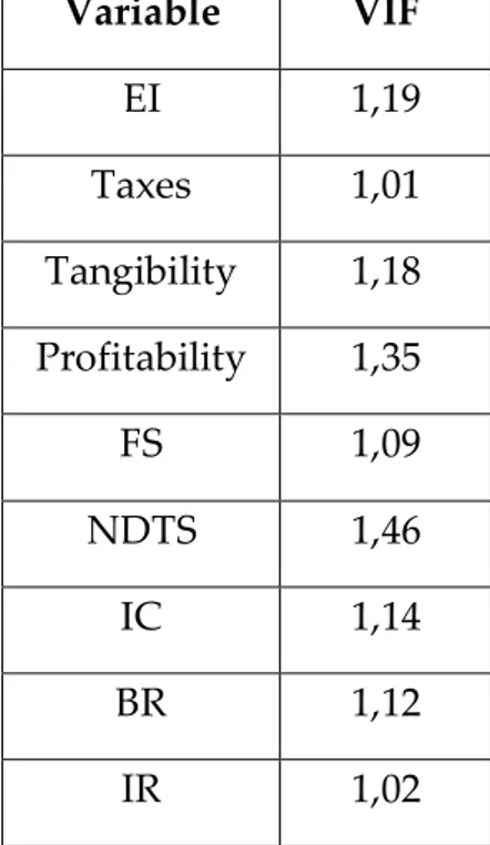
Table 1 - Summary of the variables, their measures and their expected impact on the Leverage. ... 51 Table 2 - Industry categories, corresponding SIC code and its industry code.... 53 Table 3 - Descriptive statistics before interval limitations ... 54 Table 4 - Definition of values’ intervals that the variables can assume. ... 55 Table 5 - Final table of the variables’ descriptive statistics. ... 57 Table 6 - Correlation table and the expected impact on the independent variable for each variable. ... 62 Table 7 – VIF test ... 66 Table 8 – Regression results (obtained by the Stata Software) ... 67 Table 9 - Expected signal, findings and individual significance tests for the model (1). ... 71 Table 10 - Expected signal, findings and individual significance tests for the model (2). ... 72 Table 11 - Expected signal, findings and individual significance tests for the model (3). ... 73 Table 12 - Regression results with the inclusion of the variable Growth Opportunities (obtained by the Stata software). ... 75
xv
Appendices Index
Appendix A - Median evolution of all independent variables during the 2012-2017 period ... 83 Appendix B – Correlation Tables ... 91 Appendix C – Regression results for the same model, however computed through firm fixed-effects instead of industry fixed-effects ... 93
17
Introduction
There are several capital structure theories which attempt to explain the proportions of debt and equity that firms choose. However, none of them has provide a consensual explanation of how firms finance themselves and their projects.
The pioneering work of Modigliani and Miller (1958), which presents the capital structure irrelevance theory, triggered many studies about the subject.
We decided to contribute for the extant literature by examining the financing decisions of listed Spanish firms, dividing our study into export and non-export firms, following Silva and Pinto’s (2018) suggestion to extend the study to other countries than Portugal. Before Silva and Pinto (2018), there was not any study trying to explain the differences between the exporter and non-exporter sectors, but now, with both works there is a solid basis to this subject for the Iberian Peninsula. Thus, we will search for an answer to the following two research questions: (i) What are the differences in the financing decisions between non-listed Spanish exporter and non-exporter firms? (ii) What is the impact of Export Intensity in the non-listed Spanish firms’ leverage?
Extant literature points out several theories and determinants that may influence firms’ capital structure and, consequently, their financing decisions. Modigliani and Miller (1958) present the capital structure irrelevance theory, Kraus and Litzenberger (1973) present the trade-off theory, Myers and Majluf (1984) present the pecking order theory, Baker and Wurgler (2002) present the market timing theory and Jensen and Meckling (1976) present the agency theory. Empirical literature present some determinants that are commonly used to explain firms’ capital structure, such as: Taxes [Modigliani and Miller (1963)], Tangibility [Myers (1977)], Profitability [Myers and Majluf (1984)], Firm Size [Titman and Wessels (1988)], Non-Debt Tax Shields [DeAngelo and MAsulis (1980)], Industry Conditions [Frank and Goyal (2009)], Business Risk [Bradley et
18
al. (1984)], Growth Opportunities [Myers (1977)], Inflation Rate [Gungoraydinoglu and Öztekin (2011)], and Export Intensity [Chen and Yu (2011)].
Since our focus is on the differences between the export and non-export sectors, it is important to emphasize that the existent literature on the subject is scanty and provide different results. While Chen and Yu (2011) suggests a negative relationship between export intensity and leverage, Silva and Pinto (2018) finds a positive relationship regarding exporting firms.
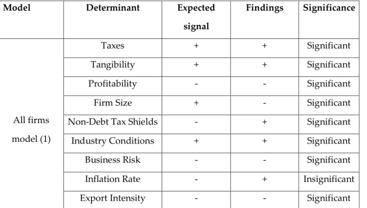
The conclusions of this study suggest that Tangibility, Profitability, Firm Size and Non-Debt Tax Shields affect the debt levels for both export and non-export firms in the same way (Tangibility and Non-Debt Tax Shields affect positively, while Profitability and Firm Size affect negatively). In addition, Taxes affects negatively leverage in the export firms and positively in the non-export firms, and Industry Conditions, Business Risk, Growth Opportunities and Inflation Rate are not significant for both type of firms. Finally, Export Intensity, within the export firms, affects positively firms’ leverage, as in Silva and Pinto (2018).
This research gives an important contribution to the literature. First, we study a country that is not normally focus by the extant literature, since most of the studies focus on US firms. Second, we analyze a sample of unlisted firms, while extant literature gives higher importance to the public/listed firms. Finally, this study presents results that are not in line with some of the major capital structure studies and is important to understand why.
This work is organized as follows. Chapter 1 presents a general framework of Spain’s macroeconomic effects. Chapter 2 presents a literature review regarding both capital structure theories and determinants. In Chapter 3 we raise the research questions and the research hypothesis that will be tested. Chapter 4 presents the variables, the sample, and both descriptive statistics and methodology used in this study. In Chapter 5 we present the regression results
19
and some robustness checks, while Chapter 6 presents the main limitations. A conclusion closes the study.
21
Chapter 1
1. General Framework
This chapter presents a Spain’s macroeconomic big picture and focus on some indicators that might be important to fully understand the concepts that we will discuss in the next chapters. All the graphs below correspond to the 2012-2017 period, which is the basis of this work.
22
1.1. Spain’s GDP
Spain is actually the fourth biggest economy in the Euro Zone and the fifth in the European Union. Exports and Imports of goods and sales have an important weight on the GDP1, being responsible for 65% of Spain’s GDP.
Graphic 1 shows that during the 2012 -2017 period the Spain’s GDP grew significantly between 2012 to 2015, whith a slightly decrease afterwards.
Graph 1 – Spain’s GDP growth rate (in percentage points) in the 2012-2017 period.
1 Gross Domestic Product is defined as an economic indicator that measures a nation’s total
23
1.2. Spain Terms of Trade
As we are studying the export sector, it is important to know if the country is accumulating more capital from exports than it is spending in imports. For that reason, the graph below shows Spain’s Terms of Trade (TOT2), which is an
important economic health indicator. However, as changes in the prices may impact this indicator, it is also important to analyze the TOT fluctuations to draw conclusions. Nevertheless, we can see in Graph 2 that during the 2012-2017 period, TOT has consistently increased, with the exception of 2017, where this indicator slightly decrease.
Graph 2 – Spain’s Terms of Trade (in percentage points) in the 2012-2017 period.
2 Terms of Trade is defined by the ratio between export and import prices. It is an indicator
that measures the country trading efficiency. If the terms of trade figures a higher percentage than 100%, means that the country exports are higher value of goods than the country imports, then the country is accumulating capital due is trading balance.
24
1.3. Spain Balance of Trade
A country’s Balance of Trade is the difference between exports and imports for a given period of time and is an important part of a nation´s current account. If a country exports more than imports, then it works on a trade surplus, otherwise it will work on a trade deficit. In graph 3, there are a lot of fluctuations during the 2012-2017 period. Spain always work on a trade deficit, however the trend is slightly positive, which means that Spain aims to have a lower trade deficit in the following years.
25
1.4. Spain Exportations
Export is when a good or service is send from one country to another to sale or trade. Exportations expands markets to global customers and boost its economies. Besides that, countries with higher value of exportations tends to grow faster than those who don’t export, once exports stimulate economic growth. Emery (1967) points out that there is a causal relationship between the increase in exports and economic growth. Through the graph 4 analysis, we can automatically understand that during the 2012-2017 period, the exports value in Spain grew very fast, with lot of fluctuations, but the trend was definitelly positive.
26
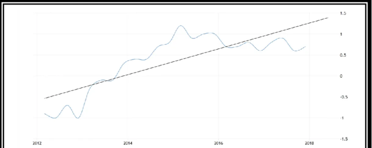
1.5. Spain Inflation Rate
Inflation Rate is one of the independent/explanatory variables of our study. The inflation rate is a measure of the rate at which the average price of a certain basket of goods and services (vary from economy to economy), increases or decreases during a certain period of time. This variable will be analyzed more deeply in the chapter 2 and 3.
By the analysis of the graph 5, we can see that at the end of 2012 this rate reaches the highest rate of the 2012-217 period with nearly 3,5%. During 2013 and 2014 there was a decreasing trend of the inflation rate, being negative during almost whole 2014. This rate keep negative during 2015 and until middle of 2016. After that, there was always a positive inflation rate until the end of 2017.
27
Chapter 2
2. Literature Review
2.1. Capital Structure Theories
Capital Structure is one of the main topics of corporate finance and is probably the one which causes more discussion when we look to the literature.
Capital Structure theories attempt to explain the right proportions of debt and equity that a firm should have. Donaldson (1952) was the first study related to capital structure, however Modigliani and Miller (1958) is considered the pioneer study in this matter, where the authors defend the capital structure irrelevance theory. This study triggered many works on the subject, such as [Kraus and Litzenberger (1973), Bradley et al. (1984), Myers and Majluf (1984), Titman and Wessels (1988), Frank and Goyal (2009)], among others.
There are a lot of theories, mainly trade-off and pecking order theories, and a lot of authors discussing different type of theories involving capital structure, however, until now, none of them provide a solid theoretical basis that can explain the financing decisions used by firms.
During this chapter, some of the main Capital Structure theories will be reviewed in order to give a comprehensive and concise approach of this major theme.
28
2.1.1. Traditional View and Irrelevance Theory
Durand (1952) was the first author that discussed this issue, arguing that it is possible to achieve an optimal capital structure, which maximizes firm value. The author points out two different approaches to measure the Capital Structure impact on the firm’s value.
The first is the Net Operating Income Method, where the firm’s value is not affected by the change in capital structure, because it undertakes the fact that a possible advantage that the firm can take from the use of debt is offset by the simultaneous increase in the bankruptcy risks that the firm may face. This annulment of benefits happens because the increase in the percentage of debt that a company holds, will lead to a higher risk of bankruptcy and such risk will, consequently, increase the risk perception of the shareholders who will demand a higher rate of return.
The second one is the Net Income Method, by which the firm’s value can increase by increasing the amount of debt. A firm should increase the weight of debt until it reaches the minimum possible WACC that the firm can achieve, and that point would be the maximization of the firm value.
The Net Income Method is in line with the traditional approach which defends that a firm must aim an optimal capital structure that minimizes the financing costs and maximizes the firm value.
Modigliani and Miller (1958) contest Durand (1952) approach by presenting the capital structure irrelevance theory. Assuming that there are no transaction costs, no bankruptcy costs, no taxes, no asymmetry information problems, no agency costs and no arbitrage opportunities, they developed to propositions. According to Proposition I, which is the one that implies the irrelevant argument, firms in the same type of business will have the same value. Therefore, the debt and equity proportion will not change the firm value. According to Proposition
29
II, the WACC is not influenced by the proportion of debt and equity that a firm have and is constant, which go against the Net Income Method proposed by Durand (1952).
Durand (1959) argues that Modigliani and Miller (1958) have jumped out of realism by overstep many assumptions. The author also says that Modigliani and Miller (1958) analyzed the risks in a very slight way and have painted the world as a remarkably safe one (without any type of risks).
Stiglitz (1969) points out an error in the Modigliani and Miller’s (1958) work. According to Stiglitz (1969), it is not possible to ignore the default risks, once the bond yield increases with firm’s leverage. Similarly, Scott (1976) asserts that the theory does not refer the dangerous effect of the unmeasured debt.
Modigliani and Miller’s (1963) paper aims to correct an existent error on their previous paper. As mentioned by the authors, “The purpose of this communication
is to correct an error in our paper "The Cost of Capital, Corporation Finance and the Theory of Investment" (this Review, June 1958)”. The authors add corporate taxes to
their model and come out with the conclusion that the firm’s value actually increases when leverage increases.
Kraus and Litzenberger (1973) relaxed the Modgliani and Miller’s (1958) model by adding bankruptcy costs. The authors argue that there is an optimal capital structure, which will origin the trade-off theory.
2.1.2. Trade-off Theory
As Modigliani and Miller (1963) point out, taxes’ advantages are in fact important and will have a huge impact on further studies. According to the authors, the proportion of debt is not related to the firm’s value, yet the authors predict that the increase of the leverage will increase the firm’s value.
30
Baxter (1967) intends to explain “in the context of the Modigliani and Miller
discussion, how excessive leverage can be expected to raise the cost of capital to the firm”.
The author argues that a firm which relies too much on debt, will increase its cost of capital. According to the author, there are a lot of costs associated with bankruptcy, and for that reason, other things equal, excess leverage might reduce the value of the firm. However, the existence of corporate taxes, which treats interest as tax deductible, suggests that leverage tend to decrease the cost of capital. In sum, according to Baxter (1967), too much leverage will increase the cost of capital, however the existence of corporate taxes will mitigate the effect.
Kraus and Litzenberger (1973) came out with the conclusion that since corporate taxes are tax deductible, a firm will only finance itself with debt in order to capture those tax advantages, although a firm should be able to pay its debt obligations, or it will face bankruptcy penalties. Kraus and Litzenberger (1973) argue that the taxation of corporate profits and the bankruptcy costs3 are
core market imperfections that must be considered in the theory of the effect of leverage on the firm’s market value. Thus, the optimal capital structure is the one where the level of debt maximizes the firm market value without lead to bankruptcy.
Kim (1978) says that the traditional presumption that the firm’s value is a concave function of its leverage and when the slope of the that function is zero, that’s where the firm’s value is maximized. According to Kim (1978), in perfect markets where there are bankruptcy costs and income taxes, the optimal level of debt of a firm is less than their debt capacities. The firm’s market value increases for low levels of debt and decreases when those firms rely too much on debt financing.
Bradley et al. (1984) develop a model where they include personal taxes, expected costs of financial distress4 and positive non-debt tax shield. They state
3 Warner (1977) distinguish direct bankruptcy costs from indirect bankruptcy costs. 4 Bankruptcy costs (see Warner 1977) and agency costs.
31
that an optimal firm capital structure is inversely related to expected costs of financial distress and non-debt tax shields.
Myers (1984) argue that an increase in the firm’s debt will lead to a risk increase and consequently will lead to an increase of the bankruptcy costs. However, this is balanced by the debt tax-shields. For this same reason, the author believe that is possible to balance a relationship between cost and benefit in order to achieve an optimal capital structure that maximizes the firm’s value. The author complements this idea in Myers (2001), by saying that firms increase their leverage until the point where the benefits of having higher levels of debt equal the possible bankruptcy and agency costs.
Static trade-off theory can be thus summarized as the perfect balance between debt and equity, under the assumption that a firm’s debt payments are tax deductible. This happens because a firm can have a lower WACC when finances itself through debt, however increasing the amount of debt also increases the bankruptcy costs.
Although there are a lot of studies that prove the importance of the Trade-off theory, there are other studies that prove that this theory is not the only one that is relevant regarding capital structure financing decisions. Fama and French (2002), point out that some relations are according to the trade-off theory (firms with more non-debt tax shields have less leverage) and some other relations are in line with the pecking order theory (more profitable firms has less leverage).
2.1.3. Pecking-order
Theory
and
Asymmetric
information
Donaldson (1961) was the first author who states that there was a pecking order of internal over external financial. The author studied some patterns of large firms and observe that the firms prioritize internal financing.
32
Later, Myers (1984) and Myers and Majluf (1984), states that financing decisions follow an order of preference and firm’s prefer internal financing over external financing, due to the asymmetric information and also the signaling problems that could arrive with external financing. The authors defend that if a firm does not have enough internal funds, it should finance through debt, depending of the costs of each source. However, a firm should always avoid to finance through external equities in order to prevent the firm’s control dilution. According to Holmes and Kent (1991), “Owner/managers are strongly adverse to any
dilution of their ownership interest and control” Holmes and Kent (1991).
In this theory there is not an optimal capital structure and each firm will choose the debt-equity ratio that perform better under the firm’s circumstances. Myers (1984) adds that a firm’s debt-equity ratio will reflect the firm external financing necessities. According to Myers (1984), a firm prefers to use retained earnings instead of finance itself by debt. Debt financing only occurs when a firm do not possess enough retained earnings.
Shyam-Sunder and Myers (1999) test the traditional capital structure approach against the pecking order model and they conclude that the pecking order model, which predicts that internal financial deficit is the main force that lead to an external financing, has much more explanatory power than a static trade-off model, which predicts that a firm adjust its capital structure in order to achieve an optimal debt-equity ratio. The authors, instead of study all the hypothesis together, like Titman and Wessels (1988) have made, they studied the theories as contending hypothesis and examined their explanatory power. Shyam-Sunder and Myers (1999) add that the strong performance of the pecking order model does not rely only on the unanticipated cash needs with debt by the firms, because indeed, according to their studies, firms plan to cover anticipated deficits with debt.
Frank and Goyal (2003) tested the model of Shyam-Sunder and Myers (1999), because the authors argued that the studied sample was too small (157 firms over
33
1971-1989 period), and they come out with the conclusion that the pecking order model does not work very well for smaller firms. However, the pecking order theory seems the one which explains better the capital structure as the firm sizes increase.
Lemmon and Zender (2010) study show that controlling the heterogeneity in debt across firms, pecking order theory describe perfectly the financing behavior of a firm.
Information asymmetries are very important when we are studying firm’s capital structure. Leland and Pyle (1977) notice that a lot of markets suffer from informational differences between the sellers and the buyers and in the financial markets, this information asymmetries are abundant. By applying this, Leland and Pyle (1977) state that in the real world, there are a lot of asymmetries between managers and shareholders. There are a lot of more information in the managers side, and for that reason, they can manipulate the shareholders by hide information for them.
According to Myers and Majluf (1984), once the investors are not fully informed as the firm insiders, equity may be mispriced by the market. This underpricing may be so severe, that can result in a net loss to the existing shareholders.
2.1.4. Market Timing theory
According to Baker and Wurgler (2002), market timing theory is defined by as
“capital structure evolves as the cumulative outcomes of past attempts to time the equity market”. They argue that there are two versions of equity market timing, being
the first one a dynamic form studied by Myers and Majluf (1984), with rational managers and investors and also adverse selection costs. The second has
34
irrational investors and perceptions of mispricing5 and suggest that firms prefer
to issue debt when the relative cost of equity is high and equity when is low. Baker and Wurgler (2002) find that when the market value is high, firms with low leverage levels tend to raise funds by selling their securities, however when the market value is low, the high leverage firm are the ones who raise funds by selling securities. Also, according to the authors, there is a negative relation between leverage and historical market valuations.
According to Frank and Goyal (2009), the basic idea of this theory is to look and understand both debt and equity market conditions. After that, if they need any financing, they will use the most favorable one. If none seems good to them, they will pass the financing need. Furthermore, if they do not need to finance but there is a funding source that is unusually favorable, this source will be used.
2.1.5. Agency theory
Following Ross (1973), the agency costs6 theory is based on the relationship
between two (or more) parties, when one (the agent) acts on behalf of the other (the principal), in a particular domain of decision making. All the contracts between two parties contain important elements of agency.
Jensen and Meckling (1976) point out that, if both parties are utility maximizers, the agent will not act on behalf of the principal every time. However, the principal can align the agent interests by establishing appropriate incentives. Nevertheless, there will be always some divergence between the agent’s decisions and the perfect decisions in the viewpoint of the principal, given the impossibility of writing complete contracts [Myers (2001)].
5 Equity is issued when managers believe its cost is irrationally low and repurchase it when
they think its cost is irrationally high.
6 Agency costs are costs that arise from inefficiency and disruption within a company and are
35
Jensen and Meckling (1976) also states that agency costs can be sum up into the following three factors: (i) monitoring costs7 by the principal; (ii) the
bonding expenditures by the agent; (iii) and the residual loss8. The authors
identify two major types of conflicts that agency costs may arise: conflicts between managers and shareholders and conflicts between shareholders and debtholders.
Jensen and Mecking (1976) described the costs that conflicts between managers and shareholders would bring to a firm. To do so, the authors compare the manager’s behavior when he owns 100% of his firm and when he sells part of firm’s shares to an outsider. When the manager owns 100% of the shares, he will make operation decisions that maximize the firm’s utility9. On the other hand,
when the manager sells part of his shares, he will stop trying to maximize firm’s utility and will try to maximize his own utility, which will put the firm’s welfare in risk. According to Jensen (1986), another conflict between managers and shareholders is related with the pay-out, since when there is conflicts between managers and shareholders, managers will prefer to invest excess cash-flow in negative NPV projects rather than see that money being distributed to the shareholders. However, Jensen (1986) says that it would be preferred that firm’s use debt as a response to the agency costs. But why? According to the author, financing through debt would obligate the managers to pay-out cash to its debtholders, otherwise the firm would face bankruptcy. This would ensure that the managers act in the best benefit to the firms.
Conflicts between shareholders and debt holders are another type of conflicts that may arise from agency costs. Myers (2001) state that they only happen when a firm face default risk. Debtholders have no interest in the firm’s
7 Not only observe the agent, but also effort in order to restrain the agent´s budget or
compensation policies.
8 Cost of the agency relationship.
9 Involves all utility aspects of a firm, such as physical appointments, attractiveness of the staff,
36
income or value when a firm it is free from default risk. Since equity is a residual claim10 when a firm faces a possible bankruptcy, shareholders will try to decrease
the value of the existing debt. Supposing that a firm is facing a significative default risk and the managers act in accordance with the shareholders, they will try to trade value from firm’s creditors to firm’s shareholders Myers (2001). Managers can shift their low-risk investments into high-risk investments, because on doing so, higher return could be captured by the shareholders, while a possible downside will be absorbed by the creditors. According to Myers (2001), Jensen and Meckling (1976) were the firsts to stresses risk-shifting as an agency problem. Borrow and pay-out cash to stockholders will also trade value, since the overall firm value will remain constant, but the debt value will decrease. This will lower the value of the shares, however the cash received will offset this loss [Myers (2001)].
2.2. Determinants of Capital Structure
Extant capital structure literature, like Harris and Raviv (1991), Rajan and Zingales (1995), Gungoraydinoglu and Öztekin (2011), Chen and Yu (2011), among others, present some factors that may influence firm’s leverage, such as: Taxes, Nature of Assets, Profitability, Firm Size, Growth Opportunities, Non-Debt Tax Shields, Industry Conditions, Business Risk, Growth Opportunities, Inflation Rate and Export Intensity. Analyze those factors is very important to understand how can they influence and why they influence the firm’s financial decisions, in certain conditions.
10 Equity claim is the right that the shareholder has to the firm’s profit, after all the obligations
37
2.2.1. Taxes
Modigliani and Miller (1963) developed the model presented in their paper of 1958 by adding the tax effect. After the inclusion of the tax effect, the authors conclude not only that firm’s value depends on leverage, but also that a firm’s value increase due to the tax benefits generated by leverage.
Baxter (1967) argues that the existence of corporate taxes, which treats interest as tax deductible, leads to the conclusion that leverage tend to decrease the cost of capital. On doing so, the existence of corporate taxes will create an optimal capital structure by balancing the costs of bankruptcy11 with the benefits from
corporate taxes. In the same line of reasoning, Kraus and Litzenberger (1973) assert that a firm should finance itself through debt in order to capture tax advantages, since taxes are deductible.
2.2.2. Nature of Assets – Tangibility
Myers (1977) suggests that for a firm which has no assets to give as a collateral, creditors will have to require more favorable conditions that the firm is not willing to accept. Hence, firms under these conditions, should prefer issuing equity rather than debt.
In line with Myers (1977), Myers and Majluf (1984) shows that the absence of tangible assets is deeply related to the information asymmetry, because a firm with less tangible assets has less collaterals to give to creditors. As tangible assets are viewed by the creditors as collaterals, firms with more tangible assets can rely more on debt since they can provide guarantees towards the debtholders. Titman and Wessels (1988) also state that the agency problem is reduced by firms that
11 Bankruptcy costs are positively related to leverage; higher debt levels will lead to higher
38
have more tangible assets, which provides them easily access to debt. For this reason, both studies draw that the relation between tangibility and leverage is positive.
Similarly, Harris and Raviv (1991) asserts that firms with comparatively less tangible assets will face more information asymmetries and, therefore, will face higher underinvestment problems.
Rajan and Zingales (1995) provide a study that aims to examine if the factors that were proven to be correlated with leverage for the United States firms are the same in the other countries, more precisely, in the G-7 countries12. As the
previous authors stated, tangible assets are easy to collateralize13 and for that
reason they reduce the agency costs of debt. This study proves that tangibility14
increase book leverage of all the countries by approximately 20% of its standard deviation, with the exception of Japan with a level of 45%.
Frank and Goyal (2009) divide assets in two major categories, tangible assets (property, plant and equipment) and intangible assets (goodwill, for example) and state that firms with more tangible assets are easier to evaluate and face less expected distress costs. So, the level of asset tangibility as well as the composition of those assets are very important in a firm’s capital structure.
However, Frank and Goyal (2009) argues that under the pecking order theory a negative relationship should be found. Low asymmetry information associated with tangible assets, will induce firms to issue equity, so a firm with more tangible assets will have lower leverage ratios. However, there is some ambiguity
12 Founded in 1975, Germany, Canada, United States, France, Italy, Japan and United Kingdom
are the group of countries that form the G-7.
13 Similarly to Rajan and Zingales (1995), Berger and Udell (1994) show that firms with close
relationships to the creditors, need to provide less collateral.
14 According to Rajan and Zingales (1995) tangibility is measure by the ratio fixed to total
39
under the pecking order theory. If there is adverse selection15 about the firms,
when tangibility increases the adverse selection will lead to a higher leverage.
2.2.3. Profitability
When we flick through the existent literature and focus on profitability, we can notice that this is a determinant that is in line with the pecking order theory. The overall results of the literature show that higher profitable firms tent to borrow less, since they will utilize internal-generated funds instead of seeking debt financing.
According to Myers (1984) and Myers and Majluf (1984), it is possible to observe a negative correlation between profitability and leverage, however, the simple explanation about this relationship resumes to the fact the equity is costly than debt, and for that reason, most profitable firms, which have internally-generated funds, tend to rely less on debt.
Jensen (1986) shows two different ways to see profitability. In the first one, there would be a positive relationship between profitability and leverage, but this only happens when there is an efficient corporate control. This corporate control will force the firm to pay out cash when leverage increases. On the other hand, if there is not an efficient corporate control, firms will present negative relationship between profitability and leverage, once they will try to stay away from the corrective role of debt.
Titman and Wessels (1988), in line with Myers (1984) and Myers and Majluf (1984) results, state that past profitability of a firm, and consequently the retained earnings available, have an important impact on the capital structure.
15 When sellers have information that buyers do not have about some aspect of the product
40
According to Rajan and Zingales (1995) profitability has a negative impact on firm’s leverage. The authors noted that larger firms tend to issue less equity and the negative impact that profitability has on leverage becomes higher as the firm sizes increases. Similar results are presented in Harris and Raviv (1991) and Frank and Goyal (2009).
2.2.4. Firm Size
Titman and Wessels (1988) find evidence in the literature that larger firms tend to rely more on debt16. The author also finds evidence in the literature17, that
relates the cost of issuing equity securities and debt with firm size. Small firms pay much more than large firms when issuing new equity and long-term debt, and for that reason, smaller firms may issue short-short term debt and become higher leveraged. This thinking is in line with the pecking order theory.
Bradley et al. (1984), Long and Malitz (1985) and Titman and Wessels (1988), also state that larger firms tend to have a larger debt-equity ratio than smaller firms. March (1982) and Rajan and Zingales (1995), also find that higher firms tend to rely more on debt.
Frank and Goyal (2009) reaches the same conclusion by saying that larger and more diversified firms face lower default risks and older firms face less debt-related agency costs. Therefore, firms which are larger and more mature tend to have higher leverage levels.
16 The author points Warner (1977) and Ang et al. (1982) as providers of such evidence. 17 Smith (1977).
41
2.2.5. Non-Debt Tax Shields
DeAngelo and Masulis (1980) point out that non-debt tax shields, as tax deductions for depreciations and investment tax credits, can be considered substitutes of the benefits which derive from debt financing. Authors also show that the relation between non-debt tax shields and firm’s leverage is negative.
On the contrary, Bradley et al. (1984) find a significant positive relationship between leverage and the level of non-debt tax shields. As pointed out by the authors, “the sign of the coefficient on non-debt tax shields is perverse” Bradley et al.
(1984).
Titman and Wessels (1988) could not confirm the significance of the relation between non-debt tax shields and leverage.
In order to take benefits of higher tax-shields, firms will issue more debt when the tax rates are higher, which will lead to a negative correlation between nondebt tax shields and leverage [Frank and Goyal (2009)]. Harris and Raviv (1991) reaches the same conclusion.
2.2.6. Industry Conditions
The Trade-Off theory predicts that higher industry median leverage should result in more leverage. Managers tend to use industry median leverage as a benchmark when they reflect about capital structure [Hovakimian et al. (2001) and Flannery and Ragan (2006)]. This means that industry median leverage is frequently used as a proxy for capital structure – firms adjust their debt to meet industry median leverage.
42
Frank and Goyal (2009), expect the same results. Authors reveal that industry effects have correlated factors18, because firms in the same industry tend to face
similar factors, like product market interactions or even competition19.
According to Frank and Goyal (2009), there are two variables that can be related to industry conditions: industry median growth and industry median leverage. Following the trade-off theory, higher industry median growth should result in less debt, while higher industry median leverage should result in higher leverage. Under the pecking order theory, industry only matter if their valuations are correlated across firms in an industry.
2.2.7. Business Risk
Volatility of firm earnings is used as a proxy for Business Risk. Bradley et al. (1984) model predicts a negative relationship between earnings volatility and firm’s leverage. Myers (1984) supports Bradley et al. (1984) prediction.
According to the trade-off theory, a firm with higher earnings volatility should have higher expected costs of financial distress and for that reason should have lower leverage [Frank and Goyal (2009)]. Frank and Goyal (2009) also stress that a firm with more volatile earnings or cash flows, will have reduced probability off having fully utilized tax shields, which leads to the conclusion that higher risk means less debt. Volatility is also linked to adverse selection. Therefore, under the pecking order theory, riskier firms have higher leverage.
18 Hovakimian et al. (2004) also follow this interpretation and included industry leverage in
their model in order to control for omitted factors.
43
2.2.8. Growth Opportunities
Myers (1977) find that profitable investment opportunities are usually discarded by most profitable firms. Rajan and Zingales (1995) say that firms that expect high future growth should finance themselves by issuing equity rather than debt when they want to finance their investments. This is in line with Myers (1977), who says that when a firm is financed with risky debt, may pass up valuable investment opportunities.
Several authors [Myers (1977), Harris and Raviv (1991), Rajan and Zingales (1995) and Frank and Goyal (2009)] support that under the trade-off theory, growth opportunities will reduce the debt-equity ratio.
Titman and Wessels (1988) did not find any reliable relation between leverage and growth opportunities.
According to Frank and Goyal (2009), under the pecking order theory, firms with more investments accumulate more debt which leads to a positive relation between growth opportunities and debt.
2.2.9. Inflation Rate
Frank and Goyal (2009) following Gertler and Gilchrist (1993), argues that not only the firm-related determinants have impact on the capital structure choices. Macroeconomic factors significantly impact firm’ s financing decisions. For example, during an expansion, stock prices usually go up and expected bankruptcy costs go down, which leads to higher borrow levels.
Agency costs, during an expansion, are likely to increase, since the managers see their wealth being reduced comparatively to shareholders’. However, if debt aligns both incentives (managers and shareholders), we should see a negative relationship between economic cycles and levels of borrow. According to the
44
pecking order theory, if during expansion periods the internal funds available are higher, firm should borrow less.
Gungoraydinoglu and Öztekin (2011) present a study that aims to deeply understand firm’s capital structure by examining both characteristics of the firm and its institutional environment. In terms of firm’s determinants, the author results are in line with both trade-off and pecking order theories.
In contrast with Frank and Goyal (2009), Gungoraydinoglu and Öztekin (2011) find a negative relation between inflation rate and leverage.
2.2.10. Exportations
According to Minetti and Zhu (2011), exporting involves a lot of initial costs and a lot of prior information in order to be successful. Das et al. (2007) assert that due to the high entry costs, which must be paid up-front, only firms with high liquidity will be able to start to export. Minetti and Zhu (2011) present results that prove that the probability of exporting is higher for firms with higher debt-equity ratios and lower cash flow20.
Chen and Yu (2011), using 566 Taiwanese firms, suggest that the relation between export intensity and leverage is negative. This relation arises from the fact that exporter firms tend to rely more on internal funds than on external financing due to the monitoring problem. According to the authors, when firms expand their operations to foreign countries, it is harder for the creditors to monitor selling activities due to its complexity. For that reason, the agency costs increase, mainly if these selling operations are on emerging economies with poor corporate governance. This will make debtholders les motivated to lend additional funds.
20 According to the author, the leverage effect could suggest that firms may use exports as a
45
Silva and Pinto (2018), using a sample of 43,078 Portuguese firms, find that export firms have a higher leverage level than non-export firms and also that among export firms, firms with higher export intensity tend to have more debt.
The literature related to exports is very scant and this is one of the main reasons that lead us to examine the impact of export intensity in capital structure and making a comparative analysis between non-listed Spanish exporter and non-exporter firms.
46
Chapter 3
3. Research Questions and Hypothesis
3.1. Research Questions
The literature review allow to build the correct framework and formulate ten research questions. Our main objective is to investigate the differences between non-listed Spanish exporter and non-exporter firms financing decisions.
On doing so, we formulate the following two research questions: (i) What are the differences in the financing decisions between non-listed Spanish exporter and exporter firms? (ii) What is the impact of Export Intensity in the non-listed Spanish firms’ leverage?
3.2. Research hypotheses
In this section, based on the determinants of firms’ leverage discussed in the section 2.2, we formulate research hypothesis. Furthermore, we will identify the proxy used, following the extant literature. Note that, we use a lot of proxies due to the difficulty of finding, in the Spanish accounting, the same items that the authors use in order to calculate the determinants.
3.2.1. Taxes
Modigliani and Miller (1963) argue that the value of a firm is not only dependent from its financing decisions, but also that tax benefits increase when firms rely more on debt. This suggests a positive relationship between corporate
47
taxes and leverage, which is supported by Baxter (1967), Kraus and Litzenberger (1973) and Gungoraydinoglu and Öztekin (2011).
As in Gungoraydinoglu and Öztekin (2011), we use the ratio between Taxes on Profits and Profits and Losses before Tax as a proxy for Taxes.
H1: There is a positive relationship between corporate taxes and leverage.
3.2.2. Tangibility
Myers (1984) and Myers and Majluf (1984) show that firms with less tangible assets is suffer more from information asymmetries. Therefore, firms with more tangible assets can rely more on debt, which can be used as collateral [Titman and Wessels (1988), Harris and Raviv (1991), Rajan and Zingales (1995) and Frank and Goyal (2009)].
Following Rajan and Zingales (1995), we use the ratio between Fixed Tangible Assets and Total Assets to calculate firm’s tangibility.
H2: Firms with more tangible assets have higher leverage.
3.2.3. Profitability
According to Myers and Majluf (1984), there is a negative relationship between profitability and the debt-equity ratio. Frank and Goyal (2009) also find a negative relationship between profitability and leverage, as well as Rajan and Zingales (1995). This expected relation is in line with the pecking order theory, since firms that are more profitable tend to finance themselves through internally generated funds.
As in Frank and Goyal (2009), the ratio between EBITDA and Total Assets is used as a proxy for firm´s profitability.
48
H3: There is a negative relationship between profitability and leverage.
3.2.4. Firm Size
According to Titman and Wessels (1988), the relation between firm size and leverage is positive. Harris and Raviv (1995) in line with Bradley et al. (1984) and Long and Malitz (1985) also state that larger firms rely more on debt. Frank and Goyal (2009) find evidence that larger and mature firms rely more on debt, since they face lower default risks and agency costs.
As in Rajan and Zingales (1995), we use logarithm of Total Assets as a proxy for firm size.
H4: Larger firms tend to rely more on debt.
3.2.5. Non-Debt Tax Shields
DeAngelo and Masulis (1980) point that non-debt tax shields can be considered substitutes of the benefits that derives from debt financing, and state that the relationship between non-debt tax shields and leverage is negative. Harris and Raviv (1991) and Frank and Goyal (2009) reach the same conclusion. As in Leary and Roberts (2005), we use the ratio between Depreciation and Total Assets as a proxy for Non-Debt Tax Shields.
H5: Firms with higher non-debt tax shields have less leverage.
3.2.6. Industry Conditions
Trade off theory predicts that higher industry median leverage should result in more leverage. Industry median leverage is usually used by the authors as a capital structure benchmark [Hovakimian et al. (2001) and Flannery and
49
Ragan (2006)]. According to Frank and Goyal (2009), higher industry median leverage should result in higher leverage.
As in Frank and Goyal (2009), we use unadjusted Median Industry Leverage as a proxy for industry conditions.
H6: There is a positive relation between Industry Leverage and firm’s leverage.
3.2.7. Business Risk
Bradley et al. (1984) predicts a negative relationship between earnings volatility (used as proxy for business risk) and leverage, which is corroborated by Myers (1984) and Myers and Majluf (1984). Frank and Goyal (2009) also expect a negative relationship, since a firm with higher earnings volatility have higher probability of financial distress costs, which may lead to lower debt levels.
We use the ratio between Enterprise Value and EBIT as a proxy for business risk.
H7: There is a negative relation between Business Risk and firm’s leverage.
3.2.8. Growth Opportunities
Rajan and Zingales (1995) argue that firms with higher future growth opportunities should obtain funding by issuing equity. Hence, firms with higher growth opportunities will have less debt levels. This is in line with Myers (1977), Harris and Raviv (1991), Fama and French (2002) and Frank and Goyal (2009). Fama and French (2002) add that a firm with high growth opportunities tend to use the retained internal cash flow in investment opportunities, which leads to small levels of debt.
50
As in Frank and Goyal (2009), we use the ratio between CAPEX and Total Assets as proxy for growth opportunities.
H8: Firms with higher growth opportunities will have less debt levels.
3.2.9. Inflation Rate
Gungoraydinoglu and Öztekin (2011) find a negative relation between inflation rate and leverage. This result is in contrast with Frank and Goyal (2009) that find a positive relation; however, the authors expect that inflation should be the least reliable factor in their study. For this reason, the negative relation found by Gungoraydinoglu and Öztekin (2011), will be our expected relation.
We use the Annual Inflation Rate as Gungoraydinoglu and Öztekin (2011), to calculate this determinant.
H9: There is a negative relationship between the annual inflation rate and leverage.
3.2.10. Exports
According to Chen and Yu (2011), firms with higher export intensity tend to have lower debt levels.
We will use the Percentage of Export Intensity as proxy for export intensity.
51
Chapter 4
4.
Variables, Sample, Descriptive Statistics and
Methodology
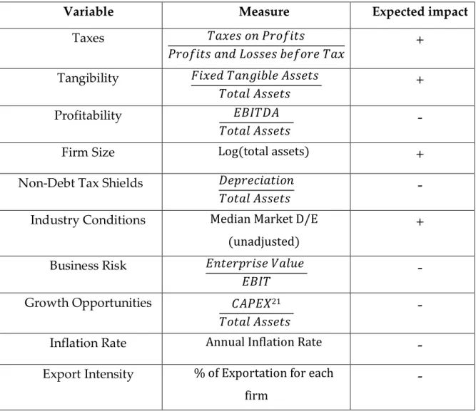
4.1. Variables
Variable Measure Expected impact
Taxes 𝑇𝑎𝑥𝑒𝑠 𝑜𝑛 𝑃𝑟𝑜𝑓𝑖𝑡𝑠 𝑃𝑟𝑜𝑓𝑖𝑡𝑠 𝑎𝑛𝑑 𝐿𝑜𝑠𝑠𝑒𝑠 𝑏𝑒𝑓𝑜𝑟𝑒 𝑇𝑎𝑥
+
Tangibility 𝐹𝑖𝑥𝑒𝑑 𝑇𝑎𝑛𝑔𝑖𝑏𝑙𝑒 𝐴𝑠𝑠𝑒𝑡𝑠 𝑇𝑜𝑡𝑎𝑙 𝐴𝑠𝑠𝑒𝑡𝑠+
Profitability 𝐸𝐵𝐼𝑇𝐷𝐴 𝑇𝑜𝑡𝑎𝑙 𝐴𝑠𝑠𝑒𝑡𝑠-
Firm Size Log(total assets)
+
Non-Debt Tax Shields 𝐷𝑒𝑝𝑟𝑒𝑐𝑖𝑎𝑡𝑖𝑜𝑛
𝑇𝑜𝑡𝑎𝑙 𝐴𝑠𝑠𝑒𝑡𝑠
-
Industry Conditions Median Market D/E
(unadjusted)
+
Business Risk 𝐸𝑛𝑡𝑒𝑟𝑝𝑟𝑖𝑠𝑒 𝑉𝑎𝑙𝑢𝑒 𝐸𝐵𝐼𝑇-
Growth Opportunities 𝐶𝐴𝑃𝐸𝑋21 𝑇𝑜𝑡𝑎𝑙 𝐴𝑠𝑠𝑒𝑡𝑠-
Inflation Rate Annual Inflation Rate
-
Export Intensity % of Exportation for each firm
-
Table 1 - Summary of the variables, their measures and their expected impact on the Leverage.
21 CAPEX is computed as fixed tangible and intangible assets for year t, less fixed tangible and
52
4.2. Sample
In order to study and compare the Spanish non-listed firm’s financing decisions for the 2012-2017 period, we selected a restricted sample of 45,147 firms (of the 1 618 332 non-listed firms that exists in Spain22). The main reason of the
decision of using only this amount of firms was that a lot of non-listed firms does not provide all the information to the database and a lot of data needed for the research was not available for the smallest companies. For that reason, we used a filter (all the companies must have in each of the 6 years of study, a value of total assets higher than 3.000.000€) in order to examine a more homogenous group of companies.
All the firm’s data used in this study were extracted from SABI Database. Additionally, the information for the variables Industry Conditions and Business Risk was taken from the DAMODARAN Website23, which provides the metrics
and the information for Industry’s means. We hand-matched firms with industries by using Industry SIC Code24.
Since we studied 45,147 firms for 6 years, we apply a panel data sample. We used the SIC Code to separate our sample by 18 different industries. Table 2 shows three columns, where the first gives the SIC Code, the second presents the industry category and the third has a code that we will use further on as Industry Fixed-Effects in our models.
22 According to SABI database at 29th of December 2018.
23 Damodaran Website is an online site, created by Aswath Damodaran who is a teacher of
corporate finance and valuation at the Stern School of Business at New York University, that among other things, provide to the user information about corporate finance and valuation metrics on industry averages.
24 SIC Code, Standard Industrial Classification Code, it is a four-digit number created by the
United States in order to facilitate the collection, presentation and the analysis of data. This code identifies the core business of any firm and covers all the economic activities.
53
Sic Code Industrial Categories IC
1. Commercial and Industrial
<=999 1.1. Agriculture, Forestry and Fishing 1
>=4812 & <=4899 1.2. Communications 2
>=1520 & <=1999 1.3. Construction/Heavy Engineer 3
1.4. Manufactoring
>=2800 & <=3099 1.1.1. Chemicals, plastic and rubber 4
>=2000 & <=2099 1.1.2. Food and Beverages 5
>=3510 & <=3872 1.1.3. Machinery and Equipments 6
>=3310 & <=3499 1.1.4. Steel, Aluminum and Other Metals 7 >=2100 & <=2799 >=3100 & <=3299 >=3873 & <=4010 1.1.5. Other 8 >=1000 & <=1310 >=1400 & <=1519
1.5. Mining and Natural Resources 9
>=1311 & <=1389 1.6. Oil and Gas 10
>=6500 & <=6999 1.7. Real Estate 11
>=5200 & <=5999 1.8. Retail Trade 12
>=7000 & <=8879 1.9. Services 13
>=5000 & <=5199 1.10. Wholesale Trade 14
>=4900 & <=4999 2. Utilities 15
>=6000 & <=6499 3. Financial Institutions 16
>=4011 & <=4811 4. Transportation 17
>=8888 & <=9729 5. Pubic Administration/Government 18
54
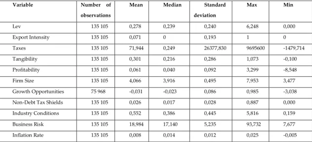
4.3. Descriptive Statistics
Table 3 presents the descriptive statistics for the dependent variable Leverage and for the explanatory variables Export Intensity, Taxes, Tangibility, Profitability, Firm Size, Non-Debt Tax Shields, Industry Conditions, Business Risk and Inflation Rate.
From now on the variable Growth Opportunities will not be part of our model since it reduces in a very significant way the number of observations. Besides that, all the statistics in the Table 3 must be read and analyzed as percentages, except the variables Firm Size, Business Risk and Inflation Rate.
Variable Number of
observations
Mean Median Standard
deviation Max Min Lev 135 105 0,278 0,239 0,240 6,248 0,000 Export Intensity 135 105 0,071 0 0,193 1 0 Taxes 135 105 71,944 0,249 26377,830 9695600 -1479,714 Tangibility 135 105 0,301 0,216 0,286 1,073 -0,100 Profitability 135 105 0,061 0,040 0,092 3,299 -8,548 Firm Size 135 105 4,066 3,916 0,495 7,953 3,477 Growth Opportunities 75 968 -0,031 -0,023 0,086 0,985 -3,038 Non-Debt Tax Shields 135 105 0,026 0,017 0,028 0,887 0,000 Industry Conditions 135 105 0,552 0,386 0,445 5,816 0,159 Business Risk 135 105 18,984 17,140 5,235 93,732 7,677 Inflation Rate 135 105 0,008 0,014 0,012 0,025 -0,005
Table 3 - Descriptive statistics before interval limitations
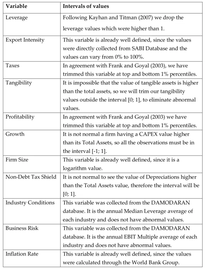
As present in the Table 3, there are some irregular/abnormal values (for example, the Taxes maximum is 9695600%). So, we create some intervals of values that the variables can assume, in order to overcome this possible problem. The intervals are presented in the Table 4.
55
Variable Intervals of values
Leverage Following Kayhan and Titman (2007) we drop the
leverage values which were higher than 1.
Export Intensity This variable is already well defined, since the values were directly collected from SABI Database and the values can vary from 0% to 100%.
Taxes In agreement with Frank and Goyal (2003), we have
trimmed this variable at top and bottom 1% percentiles. Tangibility It is impossible that the value of tangible assets is higher
than the total assets, so we will trim our tangibility values outside the interval [0; 1], to eliminate abnormal values.
Profitability In agreement with Frank and Goyal (2003) we have trimmed this variable at top and bottom 1% percentiles.
Growth It is not normal a firm having a CAPEX value higher
than its Total Assets, so all the observations must be in the interval [-1; 1].
Firm Size This variable is already well defined, since it is a logarithm value.
Non-Debt Tax Shield It is not normal to see the value of Depreciations higher than the Total Assets value, therefore the interval will be [0; 1].
Industry Conditions This variable was collected from the DAMODARAN database. It is the annual Median Leverage average of each industry and does not have abnormal values. Business Risk This variable was collected from the DAMODARAN
database. It is the annual EBIT Multiple average of each industry and does not have abnormal values.
Inflation Rate This variable is already well defined, since the values were calculated through the World Bank Group.
Table 4 - Definition of values’ intervals that the variables can assume.
After the definition of these intervals, we reached our final table of descriptive statistics (Table 5) that contain information about the Mean, Median, Standard Deviation, Maximum and Minimum of each of our variables. Besides that, in
56
order to test if the population mean ranks differ significantly between our two different populations (export and non-export firms), we run the Wilcoxon Rank Sum test. Results show that the two populations mean ranks differ significantly at the 1% significance level.
57
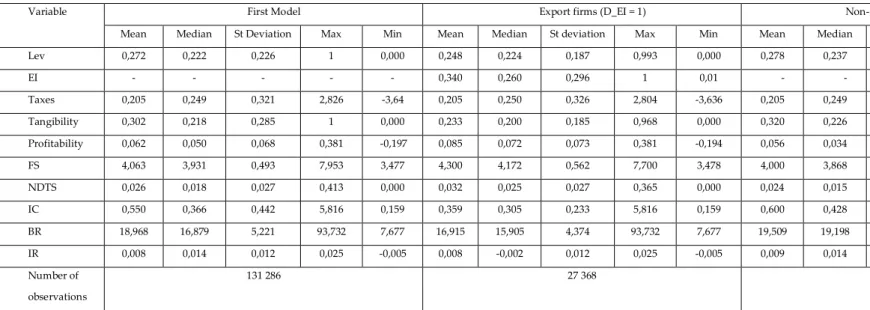
Variable First Model Export firms (D_EI = 1) Non-Export firms (D_EI = 0) Wilcoxon Test Mean Median St Deviation Max Min Mean Median St deviation Max Min Mean Median St deviation Max Min
Lev 0,272 0,222 0,226 1 0,000 0,248 0,224 0,187 0,993 0,000 0,278 0,237 0,235 1 0,000 *** EI - - - 0,340 0,260 0,296 1 0,01 - - - - Taxes 0,205 0,249 0,321 2,826 -3,64 0,205 0,250 0,326 2,804 -3,636 0,205 0,249 0,320 2,826 -3,64 *** Tangibility 0,302 0,218 0,285 1 0,000 0,233 0,200 0,185 0,968 0,000 0,320 0,226 0,304 1 0,000 *** Profitability 0,062 0,050 0,068 0,381 -0,197 0,085 0,072 0,073 0,381 -0,194 0,056 0,034 0,065 0,380 -0,197 *** FS 4,063 3,931 0,493 7,953 3,477 4,300 4,172 0,562 7,700 3,478 4,000 3,868 0,453 7,953 3,477 *** NDTS 0,026 0,018 0,027 0,413 0,000 0,032 0,025 0,027 0,365 0,000 0,024 0,015 0,027 0,413 0,000 *** IC 0,550 0,366 0,442 5,816 0,159 0,359 0,305 0,233 5,816 0,159 0,600 0,428 0,469 5,816 0,159 *** BR 18,968 16,879 5,221 93,732 7,677 16,915 15,905 4,374 93,732 7,677 19,509 19,198 5,291 93,732 7,677 *** IR 0,008 0,014 0,012 0,025 -0,005 0,008 -0,002 0,012 0,025 -0,005 0,009 0,014 0,012 0,025 -0,005 *** Number of observations 131 286 27 368 103 918
*** indicates that the population mean ranks differ significantly between export and non-export firms at the 1% significance level.
Table 5 - Final table of the variables’ descriptive statistics.
58
4.3.1. Descriptive statistics analysis
Table 5 shows that export firms have, on average, lower leverage than non-export firms. The mean (median) non-export firms’ leverage of 24,8% (22,4%) is slightly lower than non-export firms’ mean (median) leverage of 27,8% (23,7%).
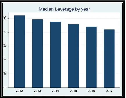
The variable Leverage decreased between 2012 to 2017, starting with a level of leverage of 26% approximately in 2012 and ending with a level of leverage of 20%, as we can see in Graph 6.