O
CTOBER
–
2018
M
ASTER
Q
UANTITATIVE
M
ETHODS FOR
D
ECISION
-
MAKING IN
E
CONOMICS AND
B
USINESS
M
ASTER
’
S
F
INAL
W
ORK
D
ISSERTATION
T
HE BANDWIDTH MINIMIZATION PROBLEM
O
CTOBER
–
2018
M
ASTER
Q
UANTITATIVE
M
ETHODS FOR
D
ECISION
-
MAKING IN
E
CONOMICS AND
B
USINESS
M
ASTER
’
S
F
INAL
W
ORK
D
ISSERTATION
T
HE BANDWIDTH MINIMIZATION PROBLEM
D
IANA
A
NDREIA DE
O
LIVEIRA
A
MARO
S
UPERVISION:
J
OÃOP
AULOV
ICENTEJ
ANELAi
Acknowledgements
First of all, I want to thank the professors and colleagues that walked with me on this journey. In particular, I want to thank my supervisors Leonor and João for their availability, knowledge and for pushing me until the end of this stage.
I also want to thank my parents for working hard so I could be focused on my studies. I‘m also very grateful for my sister that taught me the numbers and helped me with my Math homework when I was in primary school which made my love for mathematics blossom.
Lastly, I want to thank my cats for being my company despite their attempts on sitting on my keyboard and biting my computer charger.
ii
Resumo
Esta dissertação tem como objetivo comparar o desempenho de duas heurísticas com a resolução de um modelo exato de programação linear inteira na determinação de soluções admissíveis do problema de minimização da largura de banda para matrizes esparsas simétricas. As heurísticas consideradas foram o algoritmo de Cuthill e McKee e o algoritmo Node Centroid com Hill Climbing.
As duas heurísticas foram implementadas em VBA e foram avaliadas tendo por base o tempo de execução e a proximidade do valor das soluções admissíveis obtidas ao valor da solução ótima ou minorante. As soluções ótimas e os minorantes para as diversas instâncias consideradas foram obtidos através da execução do código para múltiplas instâncias e através da resolução do problema de Programação Linear Inteira com recurso ao Excel OpenSolver e ao software de otimização CPLEX. Como inputs das heurísticas foram utilizadas matrizes com dimensão entre 4 × 4 e 5580 × 5580 , diferentes dispersões de elementos não nulos e diferentes pontos de partida.
iii
Abstract
This dissertation intends to compare the performance of two heuristics with the resolution on the exact linear integer program model on the search for admissible solutions of the bandwidth minimization problem for sparse symmetric matrices. The chosen heuristics were the Cuthill and McKee algorithm and the Node Centroid with Hill
Climbing algorithm.
Both heuristics were implemented in VBA and they were rated taking into consideration the execution time in seconds, the relative proximity of the value obtained to the value of the optimal solution or lower bound. Optimal solutions and lower bounds were obtained through the execution of the code for several instances and trough the resolution of the integer linear problem using the Excel Add-In OpenSolver and the optimization software CPLEX. The inputs for the heuristics were matrices of dimension between 4 × 4 and 5580 × 5580, different dispersion of non-null elements and different initialization parameters.
iv
Table of contents
Acknowledgments ... i Resumo ... ii Abstract ... iii Table of contents ... iv Table of figures ... v Table of tables ... v Abbreviations ... vi Introduction ... 1 Literature Review ... 4 Methodology ... 7 3.1 Model ... 7 3.2 Heuristics ... 15 Computational Experiments ... 30 4.1 Instances ... 31 4.2 Computational Results ... 32 Conclusion ... 35 References ... 36 Appendix ... 397.1 Graphic representation of the problem ... 39
v
Table of figures
Figure 1 Example 1: Graph with initial model labelling... 1
Figure 2 Example 1: Alternative node labelling. ... 2
Figure 3 Tree ... 5
Figure 4 Outerplanar graph ... 5
Figure 5 Halin graph ... 5
Figure 6 Graph from Example 1. ... 9
Figure 7 Excel sheet filled with the ILP restrictions for Example 1. ... 14
Figure 8 OpenSolver window filled with the ILP parameters for Example 1. ... 14
Figure 9 Node degrees for Example 1... 21
Figure 10 Planar graph ... 39
Figure 11 Initial profile of the adjacency matrix ... 39
Figure 12 Final profile of the adjacency matrix ... 39
Figure 13 Output of OpenSolver for Example 1 ... 40
Table of tables
Table I Degree of the nodes of the non-oriented graph with 4 vertices and 5 edges ... 21Table II Table that shows the nodes assigned and not assigned for each iteration of the algorithm CM ... 22
Table III Table that shows the iterations of the heuristic NCHC ... 29
Table IV Table that contains the lower and upper bounds for each matrix used .. 31
Table V Simulation of the parameters for the NCHC algorithm ... 32
Table VI Table that makes the correspondence between the method used and its reference ... 32
vi
Abbreviations
BFS – Breadth First SearchCM – Cuthill and McKee
CPLEX – IBM ILOG CPLEX Optimization Software CSV – Comma Separated Value
FS – Feasible Solution HC – Hill Climbing
ILP – Integer Linear Programming LB – Lower Bound
MBMP – Matrix Bandwidth Minimization Problem NC – Node Centroid
NP – Non-Deterministic Polynomial Time OS – Optimal Solution
UB – Upper Bound
VBA – Visual Basic For Applications VNS – Variable Neighbourhood Search
1
Introduction
The bandwidth minimization problem has great relevance in applications because reducing the bandwidth of a matrix can, according to Chagas & De Oliveira, 2015, reduce the storage, memory consumption and processing costs of solving sparse linear systems of type 𝐴𝑥 = 𝑏, where 𝐴 is a square invertible matrix of order 𝑛 and 𝑥 and 𝑏 are vectors of dimension 𝑛.
According to Lim et al., 2004, this problem had its origin in the 1950s and it has been proven to be NP-complete by H. Papadimitriou, 1976. The bandwidth problem can also be formulated for graphs if we identify matrix 𝐴 as the corresponding adjacency matrix. In fact, Garey et al., 1978, demonstrated that even for problems where the graph’s nodes have a maximum degree of three this problem is still NP-complete.
This work intends to apply an exact Integer Linear Programming (ILP) model and two heuristics and compare their results. However, before trying to minimize the bandwidth of a matrix it is important to understand what is exactly the matrix bandwidth.
Example 1:
Taking into consideration the graph shown in Figure 1, 𝐺 = (𝑉, 𝐸) with 4 nodes, 𝑉 = {1,2,3,4} , and 5 edges, 𝐸 = {(1,2), (1,4), (2,3), (2,4), (3,4)} , we can build its adjacency matrix, where the non-null elements represent the edges of the graph. For each non-zero entry 𝑎𝑖𝑗 there is an edge connecting nodes 𝑖 and 𝑗 with weight 𝑎𝑖𝑗.
Figure 1 Example 1: Graph with initial model labelling.
1
3
4
2
2
The bandwidth of a matrix is computed from the distances of the non-null elements of the matrix to the diagonal, i.e., for row 𝑖, we determine 𝑑𝑖𝑎𝑚(𝑖) = MAX
(𝑖,𝑗)∈𝐸{|𝑖 − 𝑗|}.
In this example we get 𝐴 = [
0 1 0 1 1 0 1 1 0 1 0 1 1 1 1 0 ] ⟶ MAX{1,3} = 3 ⟶ MAX{1,1,2} = 2 ⟶ MAX{1,1} = 1 ⟶ MAX{3,2,1} = 3
, where for each
line we have recorded the maximum distance of a non-zero entry to the diagonal.
Each line of the matrix contributes with a value for the total bandwidth of the matrix 𝐴. As we can see, the first row contributes with the value 3 because the most distant non-null element from the main diagonal is located 3 indices to the right. The second row contributes with the value 2, the third row with 1 and the fourth row with 3. The bandwidth of the matrix 𝐴 corresponds to the maximum of the values contributed by each row, therefore the bandwidth of the matrix 𝐴 in this case is 3.
Since a matrix of order 𝑛 has a bandwidth at most (𝑛 − 1), the maximum bandwidth possible for a matrix is 𝑛 − 1. This means that, with the current numbering of the vertices, we obtained the maximum bandwidth for this matrix.
The bandwidth minimization problem consists in obtaining the smallest possible bandwidth by performing row and column exchanges or, in the case of graphs, by relabelling the nodes.
In this example, if we change the node labelling as shown in Figure 2, we do obtain a lower bandwidth.
Figure 2 Example 1: Alternative node labelling.
1
4
3
2
3 Adjacency matrix: 𝐴 = [ 0 1 1 0 1 0 1 1 1 1 0 1 0 1 1 0 ] ⟶ 2 ⟶ 2 ⟶ 2 ⟶ 2
As a result of the change of the numbering of the nodes, the adjacency matrix and its bandwidth were impacted. This was translated in a reduction of the bandwidth to 2 because all the rows contribute with the value 2, which in fact corresponds to the optimal solution (see appendix 7.2).
Concretely, the bandwidth minimization problem consists of permuting rows and columns of a given matrix, 𝐴 = {𝑎𝑖𝑗} , with the objective of keeping the non-null elements of a matrix as close as possible to the main diagonal. The bandwidth of A can be defined as 𝐵(𝐴) = 𝑀𝐴𝑋{|𝑖 − 𝑗|: 𝑎𝑖𝑗 ≠ 0}.
An extensive study conducted by Chagas & De Oliveira, 2015, comparing 29 metaheuristic-based heuristics showed that the four metaheuristics in the list below provided better results for the reduction of the bandwidth taking into consideration their computational cost. These heuristics are Node Centroid with Hill Climbing (Lim et al., 2004), Variable Neighbourhood Search (Mladenovic et al., 2010), Genetic Programming
Hyper-Heuristic (Koohestani & Poli, 2011) and Charged System Search (Kaveh, 2011).
Out of the four, two heuristics had low computation cost and reasonable bandwidth reduction, namely the Node Centroid with Hill Climbing and the Genetic Programming
Hyper-Heuristic. The Charged System Search heuristic had possible low computational
cost and possibly high bandwidth reduction. However, the Variable Neighbourhood
Search (VNS-band) heuristic had certainly high bandwidth reduction and reasonable
computational cost.
To give continuity to the study above, the present work intends to compare the performance of an exact method with two heuristics, that have lower computational cost: the heuristic Node Centroid with Hill Climbing (NCHC or FNC-HC) (Lim et al., 2004) and the widely used Cuthill and McKee (CM) heuristic (Cuthill & McKee, 1969).
The next part of this work will briefly refers to the available literature on this subject, mentioning applications of this problem and types of heuristics. The third part of this project will describe the exact method developed and the heuristics in a structured
4
form. The fourth part will describe how the methods were applied and will contain the computational results. Finally, the last part will address the conclusions and some reflexions about this topic.
Literature Review
The bandwidth minimization problem was originated in 1962, at Jet Propulsion Laboratory, when Harper was trying to minimize the maximum absolute error and absolute error of a 6-bit picture. This problem could be represented by a graph where the vertices were words in the code and the contribution of single errors for the total matrix bandwidth was given by the edge differences in a hypercube (Harper, 1964). This particular form of the Matrix Bandwidth Minimization Problem (MBMP) is known as the Minimum Linear Arrangement Problem.
Applications of the MBMP consist in the reduction of execution time and storage cost in the resolution of linear systems 𝐴𝑥 = 𝑏 of sparse matrices with bigger dimension. For instance, Kaveh (2004), mentioned that in structural mechanics, up to 50% of the computational cost derives from the resolution of linear systems. For instance, the computational cost of the Conjugate Gradient Method can be reduced by applying a “local” ordering of the vertices attained by implementing a heuristic that reduces the bandwidth. However, the computational cost can be higher if the bandwidth reduces too much the bandwidth (Hestenes & Stiefel, 1952). Additionally, methods that are based on the Gaussian elimination can have their number of iterations reduced just by starting with a pattern of non-zero elements in the coefficient matrix (Cuthill & McKee, 1969). Tarjan in 1975 proved that to solve a linear system with bandwidth β and 𝑛 restrictions using the Gaussian Elimination method it would require 𝒪(𝑛3) operations and fills 𝒪(𝑛𝛽2) memory space.
Many problems from physics can be described through partial differential equations for which solutions are approximated by using the finite differences, finite elements and finite volumes methods (Chagas & Oliveira, 2015). Some applications are found in chemical kinetics, survivability, numerical geophysics and large structures of transportation of energy. A concrete application is the Very Large Scale Integration,
5
which consists in the design of circuits that combine thousands of transistors or devices into a single chip (Rodriguez-Tello et al., 2008). Even in Economics, there are several models where the problems are not modelled by partial differential equations, approximations can be obtained through linearization leading to large sparse linear systems (Chagas & Oliveira, 2015). This problem was even implemented in the Computation area of hypertext layout, a particular type of data storage, by Berry et al. in 1996 when querying documents containing information from a database by matching user’s keywords to the objects of the database.
Algorithms:
There are 4 main types of resolution and approximations for this problem: exact algorithms, the first wave of heuristics, the second wave of heuristics and lower bound search.
The first type consists of exact algorithms that can only be applied to specific types of graphs with the guarantee of always finding the optimal bandwidth.
Two exact algorithms were presented in 1999 by Del Corso & Manzini can solve the MBMP for randomly generated smaller instances up to 100 vertices. As of this moment, the exact algorithm that has better performance for its worst-case scenario bases itself on dynamic programming and has complexity 𝒪(2𝑛𝑚), where 𝑚 is the number of edges and n is the number of vertices. (Koren & Harel, 2002)
For some specific graphs, there are exact methods known. For example, the tree instances which labelling can be done in polynomial time (Shiloach, 1979), some types of Halin graphs (Easton et al., 1996) and outerplanar graphs (Frederickson & Hambrusch, 1988) and others.
Figure 3 Tree Figure 4 Outerplanar graph
6
The first wave of heuristics consists of simple heuristics that provide solutions in a short amount of time sacrificing the quality.
Some examples are the CM heuristic (Cuthill & McKee, 1969) used in this work and the GPS heuristic (Gibbs et al., 1976) that are widely used as benchmarks due to its lower computation cost. However, with the increasing information obtained with the studies in this area, VNS-band (Mladenovic et al., 2010) has become more commonly used due to its good results, despite having a higher computational cost.
The second wave of heuristics can be considered the more modern ones which focus more on the quality solution over performance.
Since VNS-band has a higher computational cost and provides better solutions, it is considered to be part of the more modern heuristics. More recently, metaheuristics were constructed like for instance Tabu Search (Martı́ et al., 2001) and NCHC (Lim et al., 2004) that is presented in this work.
Finally, the fourth type is based on finding good lower bounds for the problem. Until now, the algorithms that provided Lower Bounds had an order of magnitude very inferior to the values that the heuristics obtained which made almost impossible to access the quality of the heuristics. In 2008, Martí et al., proposed exact procedures based on the Branch and Bound and Greedy Randomized Adaptive Search Procedures that computed optimal solutions for medium sized instances and lower bounds for large sized instances. Two years later, in 2011, Caprara et al., made great progress with their research by using tighter restrictions that resulted in them obtaining lower bounds with a gap generally between 5% and 20%, however, their method is very time consuming.
7
Methodology
In this section, it will be introduced an exact method for solving the minimization bandwidth problem and two heuristics that can find good solutions.
As previously mentioned, the heuristics CM and NCHC were chosen to be implemented in this work. Some factors like the availability of algorithms and examples provided by the authors were a factor in the selection of these heuristics. For instance, the heuristic CM was chosen for being a benchmark in the scientific community and for its simplicity and intuitive comprehension. NCHC was chosen because it has low computational cost but still a reasonable bandwidth reduction which makes possible its implementation in bigger problems.
3.1 Model
With the objective of obtaining an optimal solution for this problem, we present an ILP model below.
Let 𝐺(𝑉, 𝐸) be a non-oriented graph, where V is the set of vertices (or nodes), 𝑉 = {𝑣1, 𝑣2, … , 𝑣𝑛}, and E is the set of edges, 𝐸 = {𝑒1, 𝑒2, … , 𝑒𝑚}. Let 𝐴𝑛×n= {𝑎𝑖𝑗}, 𝑖 = 1, … , 𝑛; 𝑗 = 1, … , 𝑛 be the sparse symmetric adjacency matrix associated to the graph, where 𝑎𝑖𝑗 is 1 if 𝑣𝑖 is connected to 𝑣𝑗 and 0 otherwise.
Variables (𝑛2 + 1):
▪ 𝑘 = bandwidth of the matrix 𝐴 ▪ 𝑥𝑖𝑗 = {1, if the node 𝑖 is relabeled as 𝑗
0, otherwise , 𝑖, 𝑗 = 1,2, … , 𝑛
8
Restrictions (2𝑛 + number of arcs + 𝑛2):
𝑠𝑢𝑏𝑗𝑒𝑐𝑡 𝑡𝑜 { ∑ 𝑥𝑖𝑗 𝑛 𝑗=1 = 1, 𝑖 = 1, … , 𝑛 (2) ∑ 𝑥𝑖𝑗 𝑛 𝑖=1 = 1, 𝑗 = 1, … , 𝑛 (3) ∑ 𝑖(𝑥𝑢𝑖− 𝑛 𝑖=1 𝑥𝑣𝑖) ≤ 𝑘, ∀(𝑢, 𝑣): 𝑎𝑢𝑣 ≠ 0 (4) 𝑥𝑖𝑗 ∈ {0,1}, 𝑖 = 1, … , 𝑛; 𝑗 = 1, … , 𝑛 (5)
The objective function (1) minimizes the bandwidth, 𝑧 = 𝑘 , of the sparse symmetric matrix 𝐴𝑛×𝑛.
Restrictions (2) and (3) ensure that exists a bijection between the initial and final labelling of the nodes. A bijection is necessary to prevent one node from having multiple final labels or none.
Restrictions (4) establishes the link between variable k and the actual bandwidth of the adjacency matrix of the relabelled graph. In fact, if we designate by 𝜑(𝑢) the new label of the initial node 𝑢 and 𝑘 the bandwidth of the matrix 𝐴𝑛×𝑛, we have that
1. k = MAX
(𝑖,𝑗)∈𝐸{|𝑖 − 𝑗|} = MAX(𝑢,𝑣)∈𝐸{|𝜑(𝑢) − 𝜑(𝑣)|} . Therefore, because 𝐴 is symmetric, 𝜑(𝑣) − 𝜑(𝑢) ≤ 𝑘, ∀(𝑢, 𝑣): 𝑎𝑢𝑣 ≠ 0.
2. Since ∑𝑛𝑗=1𝑥𝑖𝑗 = 1 (restriction 2), the sum ∑𝑛𝑖=1𝑖. 𝑥𝑢𝑖 is reduced to one
term, 𝑖∗𝑥𝑢𝑖∗ = 𝑖∗ = 𝜑(𝑢), where 𝑖∗ is the final labelling of the node 𝑢.
3. Combining 1. and 2., we obtain the restrictions (4) that correspond to the
application of the bandwidth definition to the nodes of the graph after being relabelled.
Restrictions (5) correspond to enforce the binary nature of the variables that indicate if a node 𝑖 is relabelled as 𝑗 or not.
9
Illustration:
Figure 6 Graph from Example 1.
Writing the IPL model for Example 1 we will obtain a linear integer problem with 17 variables. Variable 𝑘 represents the final bandwidth of the matrix 𝐴4×4 and the other 16 variables represent all possible relabelling of the four nodes. For instance, node 1 can remain as 1 after the relabelling (𝑥11 = 1 ⇒ 𝑥12= 0 ⋀ 𝑥13= 0 ⋀ 𝑥14 = 0) or it can be relabelled as one of the other three nodes
𝑥𝑖𝑗 = {1, if node 𝑖 is relabeled as 𝑗
0, otherwise , 𝑖 = 1,2,3,4; 𝑗 = 1,2,3,4 (42 variables).
Since 𝑥𝑖𝑗 is a binary variable and we have four possible relabelling for each node, we obtain 16 restrictions of type (5)
𝑥𝑖𝑗 ∈ {0,1}, 𝑖 = 1,2,3,4; 𝑗 = 1,2,3,4. (5)
Furthermore, because we can only attribute the labelling of one node to another node we will have four restrictions of type (2). Also, after finalizing the relabelling, each node must have a unique label, which translates into having four restrictions of type (3)
𝑥𝑖1+ 𝑥𝑖2+ 𝑥𝑖3+ 𝑥𝑖4 = 1, 𝑖 = 1,2,3,4 (2) 𝑥1𝑗+ 𝑥2𝑗 + 𝑥3𝑗+ 𝑥4𝑗 = 1, 𝑗 = 1,2,3,4. (3)
In a symmetric matrix 𝐴4×4, each non-null element (𝑘, 𝑙) corresponds to an arc. The matrix 𝐴 has 10 non-null elements, ergo we can define the group of arcs, A, as {(1,2), (1,4), (2,1), (2,3), (2,4), (3,2), (3,4), (4,1), (4,2), (4,3)}. Therefore, representing by two opposite arcs each edges of the non-oriented graph.
1 3
4 2
10 𝐴 = [ 0 1 0 1 1 0 1 1 0 1 0 1 1 1 1 0 ] ⟶ (1,2), (1,4) ⟶ (2,1), (2,3), (2,4) ⟶ (3,2), (3,4) ⟶ (4,1), (4,2), (4,3)
To apply the bandwidth definition, the contribution of each arc doesn’t exceed the final bandwidth, 𝑘
1(𝑥𝑢1− 𝑥𝑣1) + 2(𝑥𝑢2− 𝑥𝑣2) + 3(𝑥𝑢3− 𝑥𝑣3) + 4(𝑥𝑢4− 𝑥𝑣4) ≤ 𝑘, ∀(𝑢, 𝑣): 𝑎𝑢𝑣≠ 0. (4)
Finally, the bandwidth minimization problem for the matrix 𝐴4×4 can be written as:
Variables:
▪ 𝑘 = bandwidth of the matrix 𝐴 ▪ 𝑥𝑖𝑗 = {1, if the node 𝑖 is relabeled as 𝑗
0, otherwise Objective function: 𝑚𝑖𝑛 𝑧 = 𝑘 (1) Restrictions: 𝑠𝑢𝑏𝑗𝑒𝑐𝑡 𝑡𝑜 { ∑ 𝑥𝑖𝑗 𝑛 𝑗=1 = 1, 𝑖 = 1, … , 𝑛 (2) ∑ 𝑥𝑖𝑗 𝑛 𝑖=1 = 1, 𝑗 = 1, … , 𝑛 (3) 1(𝑥11− 𝑥21) + 2(𝑥12− 𝑥22) + 3(𝑥13− 𝑥23) + 4(𝑥14− 𝑥24) ≤ 𝑘 (4.1) 1(𝑥11− 𝑥41) + 2(𝑥12− 𝑥42) + 3(𝑥13− 𝑥43) + 4(𝑥14− 𝑥44) ≤ 𝑘 (4.2) 1(𝑥21− 𝑥11) + 2(𝑥22− 𝑥12) + 3(𝑥23− 𝑥13) + 4(𝑥24− 𝑥14) ≤ 𝑘 (4.3) 1(𝑥21− 𝑥31) + 2(𝑥22− 𝑥32) + 3(𝑥23− 𝑥33) + 4(𝑥24− 𝑥34) ≤ 𝑘 (4.4) 1(𝑥21− 𝑥41) + 2(𝑥22− 𝑥42) + 3(𝑥23− 𝑥43) + 4(𝑥24− 𝑥44) ≤ 𝑘 (4.5) 1(𝑥31− 𝑥21) + 2(𝑥32− 𝑥22) + 3(𝑥33− 𝑥23) + 4(𝑥34− 𝑥24) ≤ 𝑘 (4.6) 1(𝑥31− 𝑥41) + 2(𝑥32− 𝑥42) + 3(𝑥33− 𝑥43) + 4(𝑥34− 𝑥44) ≤ 𝑘 (4.7) 1(𝑥41− 𝑥11) + 2(𝑥42− 𝑥12) + 3(𝑥43− 𝑥13) + 4(𝑥44− 𝑥14) ≤ 𝑘 (4.8) 1(𝑥41− 𝑥21) + 2(𝑥42− 𝑥22) + 3(𝑥43− 𝑥23) + 4(𝑥44− 𝑥24) ≤ 𝑘 (4.9) 1(𝑥41− 𝑥31) + 2(𝑥42− 𝑥32) + 3(𝑥43− 𝑥33) + 4(𝑥44− 𝑥34) ≤ 𝑘 (4.10) 𝑥𝑖𝑗 ∈ {0,1}, 𝑖 = 1, … , 𝑛; 𝑗 = 1, … , 𝑛 (5)
11
Model Implementation:
With the objective of implementing this methodology, it was developed a code to import a matrix and write the problem restrictions in an Excel sheet, as described in the code below. To be noted that the binary restrictions were not coded directly as they are directly inputted in OpenSolver, as it will be shown in Figure 5.
The function “OriginalMatrixReader”, shown below, is used to read a CSV file that contains the matrix 𝐴, storing its elements in the variable “OriginalMatrix”. To be noted that since the same matrices will be used with different methodologies in this work, the function “OriginalMatrixReader” will be used in the next section “3.2 Heuristics”.
Function OriginalMatrixReader() As Variant
Dim Matrix() As Integer, ColItems() As String
Dim FilePath As String, LineFromFile As String
Dim iRow As Long, iCol As integer, Number_of_Nodes As Integer
Number_of_Nodes = Sheets("Dashboard").Range("rngMatrixSize") ReDim Matrix(1 To Number_of_Nodes, 1 To Number_of_Nodes) FilePath = Sheets("Dashboard").Range("rngFilePath") Open FilePath For Input As #1
iRow = 1
Do Until EOF(1)
Line Input #1, LineFromFile
ColItems = Split(LineFromFile, ";") For iCol = 0 To UBound(ColItems)
Matrix(iRow, iCol + 1) = ColItems(iCol) Next iCol iRow = iRow + 1 Loop Close #1 OriginalMatrixReader = Matrix End Function
After reading the matrix, we sequentially implement the objective function and constraints in a format suitable to be used by OpenSolver.
12
1. Fills the first row of the Excel sheet with the list of the variables of the problem.
Cells(1, 2).Value = "k"
For i = 1 To Number_of_Nodes For j = 1 To Number_of_Nodes
Cells(1, 2 + j + (i - 1) * Number_of_Nodes) = "x" & i & "_" & j Next j
Next i
2. Writes the restrictions (2): ∑𝑛𝑗=1𝑥𝑖𝑗 = 1, 𝑖 = 1, … , 𝑛
Nb_variables = 1 + Number_of_Nodes * Number_of_Nodes iRow = 2: iCol = 2
For i = 1 To Number_of_Nodes
Cells(iRow, 1) = "SUM(xij, i=" & i & ")"
Cells(iRow, Nb_variables + 3) = "="
Cells(iRow, Nb_variables + 4) = 1
For j = 1 To Number_of_Nodes
Cells(iRow, iCol + j).Value = 1
Next j
iCol = iCol + Number_of_Nodes iRow = iRow + 1
Next i
3. Writes the restrictions (3): ∑𝑛𝑖=1𝑥𝑖𝑗 = 1, 𝑗 = 1, … , 𝑛
For j = 1 To Number_of_Nodes iCol = j + 2
Cells(iRow, 1) = "SUM(xij, j=" & j & ")"
Cells(iRow, Nb_variables + 3) = "="
Cells(iRow, Nb_variables + 4) = 1
For i = 1 To Number_of_Nodes Cells(iRow, iCol).Value = 1
iCol = iCol + Number_of_Nodes Next i
iRow = iRow + 1
13
4. Writes the restrictions (4): ∑𝑛𝑖=1𝑖(𝑥𝑢𝑖−𝑥𝑣𝑖) ≤ 𝑘, ∀(𝑢, 𝑣): 𝑎𝑢𝑣≠ 0 . To be noted that 𝑎𝑢𝑣 ≠ 0 corresponds to “OriginalMatrix(u,v)=1”
Nb_variables = 1 + Number_of_Nodes * Number_of_Nodes
For u = 1 To Number_of_Nodes For v = 1 To Number_of_Nodes
If OriginalMatrix(u, v) = 1 And u <> v Then
iCol = 2
Cells(iRow, 1) = "SUM i(xui-xvi)<=k, u=" & u & ", v=" & v Cells(iRow, Nb_variables + 3) = "<="
Cells(iRow, Nb_variables + 4) = 0
Cells(iRow, iCol).Value = -1
iCol1 = iCol + (u - 1) * Number_of_Nodes iCol2 = iCol + (v - 1) * Number_of_Nodes For i = 1 To Number_of_Nodes
Cells(iRow, iCol1 + i).Value = i Cells(iRow, iCol2 + i).Value = -i Next i
iRow = iRow + 1
End If
Next v
Next u
5. Writes the objective function, right-hand side formulas and paints the cell that contains the bandwidth function with dark orange and the cells that contain the objective variables with light orange.
' Writes the fO = k Cells(iRow, 1) = "FO" Cells(iRow, 2) = 1
' Writes the right-hand side formulas
Restriction_Variables = Cells(2, 2).Address(False, False) & ":" & _ Cells(2, Nb_variables+1).Address(False, False) Objective_Variables = Cells(iRow + 1, 2).Address & ":" & _
Cells(iRow + 1, Nb_variables + 1).Address Cells(2, Nb_variables + 2).Formula = _
"=SUMPRODUCT(" & Restriction_Variable & "," & Objective_Variables &")"
Cells(2, Nb_variables + 2).AutoFill _
Destination:=Range(Cells(2, Nb_variables + 2).Address, _ Cells(iRow, Nb_variables + 2).Address), Type:=xlFillDefault
' Paints the FO and objective variable cells
Cells(iRow, Nb_variables + 2).Interior.Color = RGB(255, 100, 0) Range(Cells(iRow + 1, 2), Cells(iRow + 1, Nb_variables + 1)) _
.Interior.Color = RGB(255, 175, 0)
14
The application of this procedure to the matrix for Example 1 yields the spreadsheet in Figure 4.
Figure 7 Excel sheet filled with the ILP restrictions for Example 1.
As previously mentioned, the binary restrictions 𝑥𝑖𝑗 ∈ {0,1}, 𝑖 = 1, … , 𝑛; 𝑗 = 1, … , 𝑛 (5) were directly inserted in the OpenSolver as per below.
15
3.2 Heuristics
Heuristic methods, from the Greek heuriskein - “to find”, have as advantages their simplicity, easy implementation and lower consumption of computational resources. As for disadvantages, they might produce low-quality solutions, depending on the initial parameters, and there is a possibility of being blocked without finding a feasible solution.
Despite having an exact compact model with a polynomial number of variables and constraints on the matrix size, heuristics are very important in finding good feasible solutions. In fact, the number of variables/ constraints has limited the study of the exact model in the section “4.2 Computational Results”. For instance, Excel has a limited number of columns that only allows the resolution of problems with the maximum dimension of 127 nodes and the time spent by OpenSolver on the resolution of bigger problems is not reasonable (more than 24h) as shown in the section “4.2 Computational Results”.
Since the objective of this work is to compare results of different methods to solve the bandwidth minimization problem, it was built the code below that calculates the bandwidth of a given matrix “MyMatrix” as per below:
𝑏𝑎𝑛𝑑𝑤𝑖𝑑𝑡ℎ = MAX
(𝑖,𝑗)∈𝐸{|𝑖 − 𝑗|} = MAX(𝑢,𝑣)∈𝐸{|𝜑(𝑢) − 𝜑(𝑣)|}
Function Calculate_Bandwidth(MyMatrix() As Integer, Phi () As Integer) Dim i As Integer, j As Integer, Band As Integer
Band = 0
For i = 1 To Number_of_Nodes For j = 1 To Number_of_Nodes
If MyMatrix(i, j) = 1 And Abs(Phi(j) – Phi (i)) > Band Then
Band = Abs(Phi (j) - Phi (i)) End If
Next j Next i
Calculate_Bandwidth = Band
16
3.2.1 The Cuthill and McKee Algorithm
The heuristic of Cuthill and McKee is a relatively simple heuristic and intends to bundle the nodes of a level with nodes of the same level, whenever possible. The levels are defined as the distance to the starting node. For instance, the adjacent nodes, also known as neighbours, of the starting node are part of the first level, the direct neighbours of the direct neighbours of the starting node are part of the second level and so on.
In the work of Cuthill and McKee is suggested to initiate the heuristic with the node of minimum degree but is also mentioned that are several cases where starting with the node of minimum degree doesn’t obtain the optimal solution. Therefore, in the section “4 Computational Experiments” this heuristic was applied with four different starting nodes: the node that has minimum degree, the node that has maximum degree, the node that has initial label 1 and the node that has initial label 𝑛.
After choosing the starting node, the remaning nodes are assigned by increasing level and, for each level, by their increasing degree.
More concretely, it was built the function “Calculate_Degree” to read the original matrix and produce a vector with the degree of each node. The degree of a node 𝑖 of 𝑑𝑒𝑔(𝑖) is the number of edges incident into 𝑖. We can determine the number of adjacent edges of 𝑖 by counting the number of edges that satisfy the condition 𝑎𝑖𝑗 = 1, which corresponds to the line of code “MyMatrix(i, j) = 1”.
Function Calculate_Degree(MyMatrix() As Integer) As Variant Dim i As Integer, j As Integer, Deg() As Integer
ReDim Deg(1 To Number_of_Nodes)
For j = 1 To Number_of_Nodes For i = 1 To Number_of_Nodes If MyMatrix(i, j) = 1 Then Deg(j) = Deg(j) + 1 End If Next i Next j Calculate_Degree = Deg End Function
17
As previously mentioned, one of the suggestions of starting node proposed by Cuthill & McKee, 1969, was to use a node that has the smallest degree. Therefore, to determine which nodes have the smallest degree it was built the function below, “Get_Random_Min_Degree”, that goes through all the elements of the vector calculated with the function presented above, “Calculate_Degree”. Since the result of heuristics depends on the starting node and it is common to have several nodes with the same degree, a random number based on the Uniform distribution was included in the function. Therefore, when there is a tie between the current node that has the minimum degree and a new node found with a minimum degree, the probability of switching is 50%.
Function Get_Random_Min_Degree(DegreeVector() As Integer) As Integer Dim Curr_Min_Degree As Integer, Curr_Node_Min_Degree As Integer Dim i As Integer
Curr_Min_Degree = Number_of_Nodes
For i = 1 To Number_of_Nodes
If DegreeVector(i) < Curr_Min_Degree Then
Curr_Node_Min_Degree = i
Curr_Min_Degree = DegreeVector(i)
ElseIf DegreeVector(i) = Curr_Min_Degree Then
If Rnd < 0.5 Then Curr_Node_Min_Degree = i End If End If Next i Get_Random_Min_Degree = Curr_Node_Min_Degree End Function
Following the same logic of “Get_Random_Min_Degree” it was built the function to obtain a node with the largest degree.
The function “Insert_Value_by_Order” will be used in this heuristic and it will be used on the NCHC heuristic. The inputs of the function are a variable “Vector_To_Update” to which will be added a value “Value” that will be inserted in a specific position according with the auxiliary value “Order_By”. In the case of the CM heuristic, the variable to be updated, list of neighbour nodes of the current node, will receive a new node “Value” and that node will be stored in a position based on its degree “Order_By”.
18
In general, the function verifies if the vector to be updated doesn’t have content “Vector_To_Update(1, 1) = 0” to access the need of creating space to receive the new “Value”. If the value to be inserted is the first one, then there is no need to check if the value that is being inserted is in the correct position as there is only one position. If the value to be inserted has the biggest “Order_By”, in the CM algorithm if it has the biggest degree, we can insert the value in the last position. Lastly, if the “Order_By”, or degree, is not the biggest of the list because we are using VBA we need to move the values to free the space where the “Value” and “Order_By” will be inserted.
Function Insert_Value_by_Order(Vector_To_Update() As Integer, Value As
Integer, Order_By As Integer) As Variant
Dim count As Integer, k As Integer
If Vector_To_Update(1, 1) = 0 Then
count = 1
Else
count = UBound(Vector_To_Update, 2) + 1
ReDim Preserve Vector_To_Update(1 To 2, 1 To count) End If
If count = 1 Then
Vector_To_Update(1, count) = Value Vector_To_Update(2, count) = Order_By
ElseIf Vector_To_Update(2, count - 1) <= Order_By Then
Vector_To_Update(1, count) = Value Vector_To_Update(2, count) = Order_By Else
k = count Do While k > 1
If Vector_To_Update(2, k - 1) > Order_By Then
Vector_To_Update(1, k) = Vector_To_Update(1, k - 1) Vector_To_Update(2, k) = Vector_To_Update(2, k - 1) k = k - 1 Else Exit Do End If Loop Vector_To_Update(1, k) = Value Vector_To_Update(2, k) = Order_By End If Insert_Value_by_Order = Vector_To_Update End Function
19
The code below starts by reading a matrix using “OriginalMatrixReader”. This matrix is then used to create the vector with the degrees of the nodes with the code specified in the previous section.
Number_of_Nodes = Sheets("Dashboard").Range("rngMatrixSize")
OriginalMatrix = OriginalMatrixReader Degree = Calculate_Degree(OriginalMatrix)
With the objective of helping to automate this heuristic, it was created a vector named “New_Nodes_Labelling” which contains the new label of the nodes. In parallel, a vector named as “Old_Nodes_Assigned” will help determine if a node has already been assigned or not during this process. This last function is very important because the same node can be a neighbour (or adjacent) of multiple nodes and we can’t relabel the same node with multiple labels. For example, having “New_Nodes_Labelling(1) = 15” means that the node that started with label 15 will be relabelled as 1. In addition, the condition “Old_Nodes_Assigned(15) = True” will be verified after the relabeling of node 15.
ReDim New_Nodes_Labelling(1 To Number_of_Nodes)
ReDim Old_Nodes_Assigned(1 To Number_of_Nodes)
Since this implementation allows the selection of a particular starting node, it was chosen to implement it with the 4 widely used starting nodes below:
1. The starting node is a node with a maximum degree
New_Nodes_Labelling(1) = Get_Random_Max_Degree(Degree)
2. The starting node is a node with a minimum degree
New_Nodes_Labelling(1) = Get_Random_Min_Degree(Degree)
3. The starting node is the first node of the matrix 𝐴
New_Nodes_Labelling(1) = 1
4. The starting node is the last node of the matrix 𝐴
20
After fixing a starting node, a search by levels for neighbour nodes that were yet not assigned will be conducted.
For each level, it will be determined the candidate nodes that were not assigned yet. These candidates verify two conditions: the first condition is that they are not assigned, i.e., the node value in the vector “Old_Nodes_Assigned” is “False” and the second condition is to be a neighbour of the “Current_Node” that has already been relabelled, i.e., “OriginalMatrix(New_Nodes_Labelling(Current_Node), iNode)” equal to “1”. All the candidates that verify these two conditions are stored in a vector named “OrderedAdj” and to ensure that they are stored by increasing order of degree it was used the function “Insert_Value_by_Order” that was presented at the beginning of this section. After having all the candidates ordered, the nodes are relabelled, i.e., they will be stored in the vector “New_Nodes_Labelling” and they will be marked as assigned to prevent them from being assigned multiple times.
This process/search will be done each node assigned until all the nodes are assigned.
Old_Nodes_Assigned(New_Nodes_Labelling(1)) = True
NbAssigned = 1: Current_Node = 1
Do While NbAssigned < Number_of_Nodes ReDim OrderedAdj(1 To 2, 1 To 1) For iNode = 1 To UBound(Degree)
If Old_Nodes_Assigned(iNode) = False And _
OriginalMatrix(New_Nodes_Labelling(Current_Node), iNode)=1 Then
OrderedAdj = Insert_Value_by_Order(OrderedAdj, iNode, _ Degree(iNode)) End If
Next iNode
' Relabels the nodes of the current adjacency by increasing degree For iNode = 1 To UBound(OrderedAdj)
NbAssigned = NbAssigned + 1
New_Nodes_Labelling(NbAssigned) = OrderedAdj(1, iNode) Old_Nodes_Assigned(OrderedAdj(1, iNode)) = True
Next iNode
Current_Node = Current_Node + 1
21
Example 1:
If we apply this heuristic to our example of the matrix 𝐴4×4, considering the starting node as the node with the smallest degree we obtain the following.
Figure 9 Node degrees for Example 1.
Node Degree (D) 1 2
2 3
3 2
4 3
Table I Degree of the nodes of the non-oriented graph with 4 vertices and 5 edges
There are two nodes with the smallest degree, 1 and 3. Therefore we can choose as starting node the node 3.
Iteration Current node
Nodes assigned
Not assigned neighbours of the current node
Candidate nodes to be assigned next
1 3 3 Level 1 = {2, 4} Level 1 = {2, 4}
Since both neighbours of node 3, 2 and 4, have the same degree, we can choose to assign the node 2.
Note: 𝒋(𝒊) indicates that node 𝒊 was relabelled as 𝒋
2 2 3, 2 Level 1 = {4}
Level 2 = {1}
Level 1 = {4}
We can only assign the node 4 because is the only node not assigned of the first level.
1 3
4 2
22
3 4 3, 2, 4 Level 2 = {1} Level 2 = {1}
Since all the nodes of the level 1 have been assigned, we proceed with adding the nodes of the second level.
4 1 3, 2, 4, 1 {} {}
The end, all the nodes have been assigned. Bandwidth before = 3
𝑴𝑨𝑿 {|𝟐 − 𝟏|, |𝟒 − 𝟏|, |𝟒 − 𝟐|, |𝟑 − 𝟐|, |𝟒 − 𝟑|} Bandwidth after = 2
𝑴𝑨𝑿 {|𝟐 − 𝟏|, |𝟑 − 𝟏|, |𝟑 − 𝟐|, |𝟒 − 𝟐|, |𝟒 − 𝟑|}
Table II Table that shows the nodes assigned and not assigned for each iteration of the algorithm CM
3.2.2 The Node Centroid with Hill Climbing Algorithm
As stated by Lim et al., 2004, in many heuristics is crucial to have a good initial solution to obtain high-quality solutions. Therefore, the NCHC algorithm starts with the generation of initial solutions by performing the Breadth First Search (BFS). Secondly, the NC is performed to centralize the positions of neighbouring nodes which is known for obtaining solutions with high quality faster than most of the recent algorithms. Lastly, the authors chose to perform the procedure HC every other time due to providing very good improvements but being relatively slow during their experimentation.
Before presenting the algorithm it is important to define the concept of a critical node. A node 𝑣 is critical if it expresses the maximum bandwidth, i.e. if the maximum distance between two nonzero elements in the corresponding row of the adjacency matrix is equal to the matrix bandwidth. When a node is critical, we define its criticality, 𝐶(𝑣), as being 1. More precisely, we set
𝐶(𝑣) = {1, 𝑖𝑓 𝑑𝑖𝑎𝑚(𝑣) = 𝑏𝑎𝑛𝑑𝑤𝑖𝑡ℎ
0, 𝑖𝑓 𝑑𝑖𝑎𝑚(𝑣) < 𝑏𝑎𝑛𝑑𝑤𝑖𝑡ℎ, where 𝑑𝑖𝑎𝑚(𝑣) = 𝑀𝐴𝑋𝑢∈𝑁(𝑣)|𝜑(𝑣) − 𝜑(𝑢)| 𝜑(𝑢) is the new label of the initial node 𝑢 and 𝑁(𝑣) = {𝑢 ∈ 𝑉: (𝑢, 𝑣) ∈ 𝐸}.
23
The NCHC algorithm is composed essentially by three other algorithms: the BFS algorithm is the first algorithm to be applied and consists in choosing randomly a starting node and adding its neighbours by levels. This is followed by the NC algorithm that adjusts the vertices to a relative central position in comparison with its neighbours (centroid) by attempting to reduce the diameter of the 𝜆 − 𝑐𝑟𝑖𝑡𝑖𝑐𝑎𝑙 vertices by moving them towards the centroid of the bundle. And finally, is then applied HC that searches for local optimal solutions based on the contribution of each node to the bandwidth, where the critical nodes that satisfy the conditions 𝐶′(𝑢) ≤ 𝐶(𝑢), 𝐶′(𝑣) ≤ 𝐶(𝑣) and 𝐶′(𝑢) + 𝐶′(𝑣) ≤ 𝐶(𝑢) + 𝐶(𝑣) are identified to perform a swap that might led to a reduction of the bandwidth; where 𝐶’(𝑣) corresponds to the criticality of the node 𝑣 after the swap, considering the current bandwidth.
The algorithm starts by reading the inputs such as the number “restart_Times”, that corresponds to the number of times that the algorithm will restart by generating new initial solutions, the “NC_Times” that corresponds to the number of times that the NC algorithm will be performed, “lambda” that is the factor that will be applied to the bandwidth of the matrix in order to obtain the 𝜆 − critical vertices and the matrix to be used.
restart_Times = Sheets("Dashboard").Range("rngRestart_Times") NC_Times = Sheets("Dashboard").Range("rngNC_Times")
lambda = Sheets("Dashboard").Range("rng_lambda")
Number_of_Nodes = Sheets("Dashboard").Range("rngMatrixSize") OriginalMatrix = OriginalMatrixReader
The variable “CurBandwidth”, that represents the minimum bandwidth at any given step of the heuristic, was added to the original algorithm to store the bandwidth obtained at the end of performing the HC algorithm and before labels being reset by the function “IntialLabels” (BFS algorithm).
CurBandwidth = Number_of_Nodes
For i = 1 To restart_Times
Labelling = InitialLabels(OriginalMatrix) For j = 1 To NC_Times
Labelling = NC(OriginalMatrix, Labelling, lambda) If j Mod 2 = 1 Then
Labelling = HC(OriginalMatrix, Labelling) End If
Next j
If CurBandwidth > Bandwidth Then CurBandwidth = Bandwidth
24
The function “InitialLabels” performs the algorithm BFS, which consists in choosing randomly a starting node and adding its neighbours by levels. This algorithm is very similar to what was used in the CM algorithm as it considers the neighbourhood of a node but doesn’t relabel it by increasing degree.
Function InitialLabels(OriginalMatrix() As Integer) ReDim New_Nodes_Labelling(1 To Number_of_Nodes) ReDim Old_Nodes_Assigned(1 To Number_of_Nodes)
New_Nodes_Labelling(1) = Int(Number_of_Nodes * Rnd + 1) Old_Nodes_Assigned(New_Nodes_Labelling(1)) = True
NbAssigned = 1: CurrNode = 1
Do While NbAssigned < Number_of_Nodes For iNode = 1 To Number_of_Nodes
If Old_Nodes_Assigned(iNode) = False And _
OriginalMatrix(New_Nodes_Labelling(CurrNode), iNode) = 1 Then
NbAssigned = NbAssigned + 1 New_Nodes_Labelling(NbAssigned) = iNode Old_Nodes_Assigned(iNode) = True End If Next iNode CurrNode = CurrNode + 1 Loop InitialLabels = New_Nodes_Labelling End Function
25
After relabelling the nodes in the step before there is a need to recalculate the bandwidth to be able to sort the nodes according to their weight, from smallest to largest using the NC algorithm. The weight of each node depends on its contribution to the final bandwidth, being the weight of each node defined as 𝑤(𝑣) =∑𝑢∈𝑏𝜆(𝑣)𝑓(𝑢)
|𝑏𝜆(𝑣)| , for which
𝑏𝜆(𝑣) = {𝑁(𝑣) ∩ {𝑢: |𝑓(𝑢) − 𝑓(𝑣)| ≥ 𝜆𝐵(𝐺)} ∪ {𝑣}, where 𝑁(𝑣) is the neighbourhood of 𝑣, 𝐵(𝐺) is the bandwidth of the graph 𝐺 and 𝑓(𝑢) is the label of the initial node 𝑢.
Function NC(OriginalMatrix() As Integer, Labelling() As Integer, lambda
As Double)
Bandwidth = Calculate_Bandwidth(OriginalMatrix, Labelling) ReDim C(1 To Number_of_Nodes) ReDim w(1 To Number_of_Nodes) For i = 1 To Number_of_Nodes w(i) = Labelling(i) C(i) = 1 Next i For u = 1 To Number_of_Nodes For v = 1 To Number_of_Nodes If OriginalMatrix(u, v) = 1 And _
Abs(Labelling(u) - Labelling(v)) >= lambda * Bandwidth Then
w(u) = w(u) + Labelling(v): C(u) = C(u) + 1
w(v) = w(v) + Labelling(u): C(v) = C(v) + 1 End If Next v Next u For i = 1 To Number_of_Nodes w(i) = w(i) / C(i)
Next i
For u = 1 To Number_of_Nodes - 1
For v = u + 1 To Number_of_Nodes If w(u) > w(v) Then
temp = w(u): w(u) = w(v): w(v) = temp temp = Labelling(u) Labelling(u) = Labelling(v) Labelling(v) = temp End If Next v Next u NC = Labelling End Function
26 )
Before presenting the HC algorithm is important to mention that the function 𝐶(𝑣) is used with the name “Critical”, the function 𝑑𝑖𝑎𝑚(𝑣) is mentioned by the name “Diam” and the function “Neighbours” corresponds to the neighborhood of a node. It is also used the function “NeighboursLine” that corresponds to the neighbours of the node 𝑣, 𝑁(𝑣), that are closer to the 𝑚𝑖𝑑(𝑣) than to 𝜑(𝑣). This group is sorted by increasing order of |𝑚𝑖𝑑(𝑣) − 𝜑(𝑢)| and is represented by 𝑁′(𝑣) = {𝑢: |𝑚𝑖𝑑(𝑣) − 𝜑(𝑢)| < |𝑚𝑖𝑑(𝑣) − 𝜑(𝑣)|, where 𝑚𝑖𝑑(𝑣)⌊= (𝑀𝐴𝑋{𝜑(𝑢): 𝑢 ∈ 𝑁(𝑣)} + 𝑚𝑖𝑛{𝜑(𝑢): 𝑢 ∈ 𝑁(𝑣)})/2⌋.
Function NeighboursLine(v As Integer, Matrix() As Integer) N = Neighbours(v, Matrix)
max_label_v = 0: min_label_v = Number_of_Nodes For i = 1 To UBound(N)
If Labelling(N(i)) > max_label_v Then _
max_label_v = Labelling(N(i)) If Labelling(N(i)) < min_label_v Then _
min_label_v = Labelling(N(i)) Next i
mid_label_v = Int((max_label_v + min_label_v) / 2)
ReDim Naux(1 To 2, 1 To 1) For Each u In N
If Abs(mid_label_v - Labelling(u)) < _ Abs(mid_label_v - Labelling(v)) Then
Naux = Insert_Value_by_Order(Naux, CInt(u), _ Abs(mid_label_v - Labelling(u))) End If Next u NeighboursLine = Naux End Function
27
Finally, the algorithm HC is applied. This algorithm searches for local optimal solutions based on the contribution of each node to the bandwidth.
In this algorithm, critical nodes that satisfy the conditions 𝐶′(𝑢) ≤ 𝐶(𝑢), 𝐶′(𝑣) ≤ 𝐶(𝑣) and 𝐶′(𝑢) + 𝐶′(𝑣) ≤ 𝐶(𝑢) + 𝐶(𝑣) are identified to perform a swap that might led to a reduction of the bandwidth; where 𝐶’(𝑣) corresponds to the criticality of the node 𝑣 after the swap, considering the current bandwidth. To be noted that only for the HC, 𝐶’(𝑣) can also have a value of 2 if the swap leads to an increase in the bandwidth, i.e., if we would obtain 𝑑𝑖𝑎𝑚(𝑣) > 𝑏𝑎𝑛𝑑𝑤𝑖𝑑𝑡ℎ after the swap. A detailed demonstration can be found in the work of Lim et al., 2004.
Function HC(OriginalMatrix() As Integer, Labelling() As Integer) ReDim C(1 To Number_of_Nodes)
ReDim CLine(1 To Number_of_Nodes)
Bandwidth = Calculate_Bandwidth(OriginalMatrix, Labelling) can_improve = True
Do While can_improve = True
can_improve = False
For v = 1 To Number_of_Nodes
C(v) = Critical(v, OriginalMatrix, Labelling) If C(v) = 1 Then
NLine = NeighboursLine(v, OriginalMatrix) If NLine(1, 1) <> 0 Then For uu = 1 To UBound(NLine, 2) u = NLine(1, uu) LabellingLine = Labelling LabellingLine(v) = Labelling(u) LabellingLine(u) = Labelling(v)
C(u) = Critical(u, OriginalMatrix, Labelling)
If Diam(v, OriginalMatrix, LabellingLine) > Bandwidth Then
CLine(v) = 2
Else
CLine(v) = Critical(v, OriginalMatrix, LabellingLine) End If
If Diam(u, OriginalMatrix, LabellingLine) > Bandwidth Then
CLine(u) = 2
Else
CLine(u) = Critical(u, OriginalMatrix, LabellingLine) End If
28
If CLine(u) <= C(u) And CLine(v) <= C(v) And _ CLine(u) + CLine(v) < C(u) + C(v) Then
Labelling = LabellingLine
Bandwidth =Calculate_Bandwidth(OriginalMatrix,Labelling) can_improve = True: Exit For
End If Next uu End If End If Next v Loop HC = Labelling End Function
If we apply this heuristic to the example below with the parameters “restart_Times=1”, “NC_Times=1” and “lambda=0,7” we obtain the following table.
𝐴 = [ 0 1 1 1 1 0 1 0 1 0 0 0 1 1 0 1 0 0 1 0 1 0 0 1 1 0 0 0 0 1 0 0 0 1 1 0] Iteration Current node
Labelling Not assigned neighbours of the current node
Candidate nodes to be assigned next BFS 5 5 Level 1 = {1,6} Level 1 = {1,6} 5 5,1 Level 1 = {6} Level 1 = {6} 1 5,1,6 Level 2 = {2,3,4} Level 2 = {2,3,4} 1 5,1,6,2 Level 2 = {3,4} Level 2 = {3,4} 1 5,1,6,2,3 Level 2 = {4} Level 2 = {4} 6 5,1,6,2,3,4 {} {} NC Labelling={5,1,6,2,3,4} ; Bandwidth=4
Note: For w(i) and c(i), i represents the relabelled node. Therefore, w(1) is
the weight of the node with label 5. w(1)=7 ; c(5)=3 => w(1)/c(1)=2,(3) w(2)=23 ; c(2)=5 => w(2)/c(2)=4,6 w(3)=12 ; c(3)=5 => w(3)/c(3)=2,4 w(4)=14 ; c(4)=3 => w(4)/c(4)=4,(6)
29 w(5)=3 ; c(4)=1 => w(5)/c(5)=3 w(6)=4 ; c(4)=1 => w(6)/c(6)=4
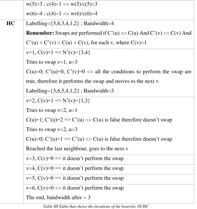
HC Labelling={5,6,3,4,1,2} ; Bandwidth=4
Remember: Swaps are performed if C’(u) <= C(u) And C’(v) <= C(v) And
C’(u) + C’(v) < C(u) + C(v), for each v, where C(v)=1 v=1, C(v)=1 => N’(v)={3,4}
Tries to swap v=1, u=3
C(u)=0; C’(u)=0, C’(v)=0 => all the conditions to perform the swap are true, therefore it performs the swap and moves to the next v
Labelling={3,6,5,4,1,2} ; Bandwidth=3 v=2, C(v)=1 => N’(v)={1,3}
Tries to swap v=2, u=1
C(u)=1; C’(u)=2 => C’(u) <= C(u) is false therefore doesn’t swap Tries to swap v=2, u=3
C(u)=0; C’(u)=1 => C’(u) <= C(u) is false therefore doesn’t swap Reached the last neighbour, goes to the next v
v=3, C(v)=0 => it doesn’t perform the swap v=4, C(v)=0 => it doesn’t perform the swap v=5, C(v)=0 => it doesn’t perform the swap v=6, C(v)=0 => it doesn’t perform the swap The end, bandwidth after = 3
30
Computational Experiments
In this section the results will be compared taking into consideration the time of execution in seconds, the relative proximity of value of the Feasible Solution (FS) to the value of the Optimal Solution (OS)/ Lower Bound (LB), (FS-LB)/LB and the relative bandwidth reduction (final bandwidth-initial bandwidth)/initial bandwidth).
Below are the technical details of the computer used to test the heuristics and the exact model with OpenSolver:
▪ Processor: Intel(R) Core(TM) i3-2350M CPU @ 2.30GHz ▪ Video Card: Intel(R) HD Graphics 3000
▪ Video Card #2: NVIDIA GeForce 610M ▪ RAM: 6.0 GB
▪ Operating System: Microsoft Windows 10 (build 16299), 64-bit ▪ Software used: Microsoft Excel for Office 365 MSO 64-bit
31
As mentioned by Cuthill & McKee, 1969, a Lower Bound (LB) for the heuristics can be the smallest integer that is greater or equal to 𝐷/ 2, where 𝐷 is the maximum degree of any node of the graph.
𝒏 LB = ⌈𝑫/𝟐⌉ UB = lowest bandwidth found 4 2 2 18 3 5 36 3 6 102 4 14 354 4 269 679 4 537 695 4 543 1255 4 1097 1845 4 1510 2092 4 1776 2772 4 2335 3463 4 2973 3669 4 3637 4761 4 4711 5580 5 4710
Table IV Table that contains the lower and upper bounds for each matrix used
As seen in Table IV, the LB presented is poor for matrices of bigger dimension, an increase of a matrix dimension by 5577 only leads to an increase of 1 in the LB.
4.1 Instances
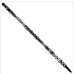
We will use sparse symmetric matrices of dimension 4, 18, 36, 102, 354, 679, 695, 1255, 1845, 2092, 2772, 3463, 3669, 4761 and 5580 as inputs for the exact model and for the heuristics. These matrices were generated from regular conform triangulations of fixed 2-dimensional domains relevant in solution of elliptic partial differential equations. To avoid mesh distortion, all the triangles are close to equilateral, which in turn fixes the typical degree of any node to be 6 for internal nodes and 4 for boundary nodes (see Figure 10).
To help determine the fixed parameters of the heuristic NCHC, it was chosen the matrix 36 × 36 to perform a simulation with fifty repetitions, 𝑟𝑒𝑠𝑡𝑎𝑟𝑡_𝑡𝑖𝑚𝑒𝑠, for each 𝜆 and 𝑁𝐶 𝑡𝑖𝑚𝑒𝑠 on the table below. As can be seen in the table below, the parameters that
32
will be used are λ=0,7 and 𝑁𝐶 𝑡𝑖𝑚𝑒𝑠 = 15. Due to this algorithm being slow, the number of 𝑟𝑒𝑠𝑡𝑎𝑟𝑡_𝑡𝑖𝑚𝑒𝑠 that will be used is 5.
𝝀 NC times 0 0,25 0,5 0,7 0,8 0,9 0,95 1 3 18 17 17 21 20 21 22 26 5 21 18 19 18 19 20 22 26 7 17 20 19 18 21 19 19 26 11 19 20 18 20 20 21 20 26 15 18 21 19 15 20 21 22 26
Table V Simulation of the parameters for the NCHC algorithm
To refer to each method on the right side of the table we will use the reference on the left side.
Reference Method
OS Open Solver
CPLEX CPLEX
CM_SD CM – start on the node with the smallest degree
CM_LD CM – start on the node with the largest degree
CM_1N CM – start on the 1st node
CM_LN CM – start on the last node
NCHC NCHC restarting 5 times, performing NC 15 times and with 𝜆 = 0,7
Table VI Table that makes the correspondence between the method used and its reference
4.2 Computational Results
To better compare the results the matrices were split into 3 groups. The smallest group is composed by the matrices which we can use the model in Excel due to columns limitation, which is reflected in a limited number of variables. These matrices have a dimension smaller than 128 nodes (4, 18, 36, 102). The second group will contain medium sized matrices with a dimension between 128 and 2000 (354, 679, 695, 1255, 1845).
33
Lastly, the group with large matrices will contain matrices with dimension greater than 2000 (2092, 2772, 3463, 3669, 4761, 5580).
To be noted that due to the extensive time that the exact model take to achieve an optimal solution, it was decided to limit their running time to 24 hours, 86400 seconds.
Small matrices: 4,18,36,102
Reference Average time spent (sec.)
Relative proximity to OS/ LB (smaller is better) Relative bandwidth (smaller is better) OS* 45517 76,79% -55,57% CPLEX* 21616 0,00% -67,44% CM_SD 0 326,79% -1,56% CM_LD 0 326,67% -0,21% CM_1N 0 305,36% -11,16% CM_LN 0 331,79% 0,00% NCHC 0,25 178,57% -29,83%
*Note: Despite using the exact model, the time of the execution was capped at 24h
per matrix which led to a difference in the relative bandwidth after the application of the model.
Medium matrices: 354, 679, 695, 1255, 1845
Reference Average time spent (sec.)
Relative proximity to OS/ LB (smaller is better) Relative bandwidth (smaller is better) CM_SD 1,1 22,48% 0,35% CM_LD 1,1 23,22% 0,94% CM_1N 1,1 23,49% 1,19% CM_LN 1,1 23,35% 1,08% NCHC 855,6 0,00% -17,88%
34
Large matrices: 2092, 2772, 3463, 3669, 4761 and 5580
Reference Average time spent (sec.)
Relative proximity to OS/ LB (smaller is better) Relative bandwidth (smaller is better) CM_SD 6,8 17,28% 0,16% CM_LD 6,8 17,18% 0,08% CM_1N 6,8 17,35% 0,22% CM_LN 6,8 17,34% 0,21% NCHC 12806,3 0,00% -14,56%
Based on the tables above we can conclude that bigger matrices require more time to have their bandwidth reduced. This is in line with what was expected since the heuristics take more to read the matrices and there are more possibilities of columns and rows permutations that can potentially lead to the maximum bandwidth reduction. This is also verified in the resolution of the exact model as there are more restrictions. For instance, for the matrix of dimension 106, it was not found an optimal solution in less than 24h using the exact model.
The CM proved to be an algorithm with an easy and intuitive implementation that provides results in a short period of time. However, it doesn’t reduce the bandwidth as much as the NCHC algorithm and in some cases, the bandwidth even increases, despite different starting points being considered. Regardless, for the smaller matrices, the bandwidth resultant of the application of the algorithm NCHC is half as good as the exact model which indicates that there is room for improvement and creation of new heuristics.
35
Conclusion
Several constraints were faced during this study. On the resolution with the exact method, it was verified that Excel has a low number of columns (16.384) which restrained the dimension of the matrices that could be solved with the exact method to 127 × 127. Also, even when it was possible to generate the restrictions to input in OpenSolver, it was verified that for dimensions 36 and 102 OpenSolver couldn’t reach an optimal solution. CPLEX performed better in comparison as it was able to reach the optimal solution for the matrix with dimension 36 and good UB for the bandwidth of the matrix with dimension 102.
It was noticed that the NCHC heuristic performed very slowly in comparison with the heuristic CM, but it obtained a better UB for the bandwidth’s matrices. This difference in computation time is related to the complexity of the NCHC heuristic and the inefficiency of VBA to handle calculations and sorts on matrices with big dimensions.
It was also concluded that the relative bandwidth reduction obtained with the CM heuristic was inferior to the one obtained with the NCHC heuristics, having matrices where the bandwidth increased after performing the algorithm CM. As a consequence of having a greater bandwidth reduction for the instances used, the algorithm NCHC was always closer to the LB than the algorithm CM.
36
References
Berry, M.W., Hendrickson, B. & Raghavan, P. (1996). Sparse matrix reordering schemes for browsing hypertext. Lect. Appl. Math. 32. p.pp. 99–123.
Caprara, A., Letchford, A.N. & Salazar-González, J.-J. (2011). Decorous Lower Bounds for Minimum Linear Arrangement. INFORMS Journal on Computing. [Online]. 23
(1). p.pp. 26–40. Available from:
http://pubsonline.informs.org/doi/abs/10.1287/ijoc.1100.0390.
Chagas, G.O. & Oliveira, S.L.G. de (2015). Metaheuristic-based Heuristics for Symmetric-matrix Bandwidth Reduction: A Systematic Review. Procedia
Computer Science. [Online]. 51 (1). p.pp. 211–220. Available from:
http://dx.doi.org/10.1016/j.procs.2015.05.229.
Del Corso, G.M. & Manzini, G. (1999). Finding Exact Solutions to the Bandwidth Minimization Problem. Computing. [Online]. 62 (3). p.pp. 189–203. Available from: https://doi.org/10.1007/s006070050002.
Cuthill, E. & McKee, J. (1969). Reducing the Bandwidth of Sparse Symmetric Matrices. In: Proceedings of the 1969 24th national conference of the ACM. [Online]. 1969, New York, New York, USA: ACM Press, pp. 157–172. Available from: https://doi.org/10.1145/800195.805928.
Easton, T., Horton, S. & Parker, R.G. (1996). A solvable case of the linear arrangement problem on Halin graphs. Congressus Numerantium. 119.
Frederickson, G.N. & Hambrusch, S.E. (1988). Planar linear arrangements of outerplanar graphs. IEEE Transactions on Circuits and Systems. 35 (3). p.pp. 323–333.
Garey, M.R., Graham, R.L., Johnson, D.S. & Knuth, D.E. (1978). Complexity Results for Bandwidth Minimization. SIAM Journal on Applied Mathematics. [Online]. 34 (3). p.pp. 477–495. Available from: https://doi.org/10.1137/0134037.
Gibbs, N.E., Poole, W.G. & Stockmeyert, P.K. (1976). An algorithm for reducing the bandwith and profile of a sparse matrix. SIAM Journal on Numerical Analysis. [Online]. 13 (2). p.pp. 236–250. Available from: http://dx.doi.org/10.1137/0713023. Harper, L. (1964). Optimal Assignments of Numbers to Vertices. Journal of the Society
for Industrial and Applied Mathematics. [Online]. 12 (1). p.pp. 131–135. Available
from: https://doi.org/10.1137/0112012.