J. Braz. Comp. Soc. vol.15 número2

(1)

*e-mail: ricardo@dc.ufscar.br

The impact of spatial data redundancy on SOLAP

query performance

Thiago Luís Lopes Siqueira

1,2

_{, Cristina Dutra de Aguiar Ciferri}

3

_{, Valéria Cesário Times}

4

_,

Anjolina Grisi de Oliveira

4

_{, Ricardo Rodrigues Ciferri}

1

_*

1_{Computer Science Department, Federal University of São Carlos – UFSCar}

13565-905, São Carlos, SP, Brazil

2_{São Paulo Federal Institute of Education, Science and Technology – IFSP Salto Campus}

13320-271, Salto, SP, Brazil

3_{Computer Science Department – ICMC, University of São Paulo – USP}

13560-970, São Carlos, SP, Brazil

4_{Informatics Center, Federal University of Pernambuco – UFPE}

50670-901, Recife, PE, Brazil

A previous version of this paper appeared at GEOINFO 2008 (X Brazilian Symposium on Geoinformatics) Received: March 10, 2009; Accepted: May 12, 2009

Abstract: Geographic Data Warehouses (GDW) are one of the main technologies used in decision-making processes and spatial

analysis, and the literature proposes several conceptual and logical data models for GDW. However, little effort has been focused on studying how spatial data redundancy affects SOLAP (Spatial On-Line Analytical Processing) query performance over GDW. In this paper, we investigate this issue. Firstly, we compare redundant and non-redundant GDW schemas and conclude that redundancy is related to high performance losses. We also analyze the issue of indexing, aiming at improving SOLAP query performance on a redundant GDW. Comparisons of the SB-index approach, the star-join aided by R-tree and the star-join aided by GiST indicate that the SB-index significantly improves the elapsed time in query processing from 25% up to 99% with regard to SOLAP queries defined over the spatial predicates of intersection, enclosure and containment and applied to roll-up and drill-down operations. We also investigate the impact of the increase in data volume on the performance. The increase did not impair the performance of the SB-index, which highly improved the elapsed time in query processing. Performance tests also show that the SB-index is far more compact than the star-join, requiring only a small fraction of at most 0.20% of the volume. Moreover, we propose a specific enhancement of the SB-index to deal with spatial data redundancy. This enhancement improved performance from 80 to 91% for redundant GDW schemas.

Keywords: geographic data warehouse, index structure, SOLAP query performance, spatial data redundancy.

1. Introduction

Although Geographic Information Systems (GIS), Data Warehouse (DW) and On-Line Analytical Processing (OLAP) have different purposes, all of them converge in one aspect: decision-making support. Some authors have already proposed they be integrated in a Geographic Data Warehouse (GDW) to provide a means for carrying out spatial analyses combined with agile and flexible multidimensional analytical queries over huge data volumes6, 14, 26, 27_{. However, little effort}

has been devoted to investigating the following issue: How does spatial data redundancy affect query response time and storage requirements in a GDW?

Similarly to a GIS, a GDW-based system manipulates geographic data with geometric and descriptive attributes, and also supports spatial analyses and ad hoc query windows. Like a DW12_{, a GDW is a subject-oriented, integrated,}

time-variant and non-volatile dimensional database, which is often organized in a star schema with dimension and fact tables. A dimension table contains descriptive data and

is typically designed in hierarchical structures in order to support different levels of aggregation. A fact table addresses numerical, additive and continuously valued measuring data, and maintains dimension keys at their lowest granu-larity level and one or more numeric measures as well. In fact, a GDW stores geographic data in one or more dimen-sions or in at least one measure of the fact table6, 14, 26, 27, 30_{. An}

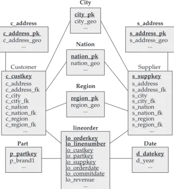
example of star-schema with spatial attributes is shown in Figure 1 (Section 4.1).

While OLAP is the technology that provides strategic multidimensional queries over the DW, spatial OLAP (SOLAP) provides analytical multidimensional queries based on spatial predicates that mostly run over GDW2, 6, 12, 25, 27_.

Typical types of spatial predicates are intersection, enclo-sure and containment7_{. The spatial query window is often an} ad hoc area, not predefined in the spatial dimension tables.

(2)

executing roll-up and drill-down operations. These OLAP operations perform data aggregation and disaggregation, according to higher and lower granularity levels, respectively. Kimball and Ross12_{stated that a redundant DW schema is}

preferable to a non-redundant one, since the former does not introduce new join costs and the attributes assume conven-tional data types that require only a few bytes. On the other hand, in GDW it may not be feasible to estimate the storage requirements for a spatial object represented by a set of geometric data30_{. Also, evaluating a spatial predicate is much}

more expensive than executing a conventional one7_.

Hence, choosing between a redundant and a non-redun-dant GDW schema may not lead to the same option as for conventional DW. This indicates the need for an experimental evaluation approach to aid GDW designers in making this choice. In this paper, we investigate spatial data redundancy effects in SOLAP query performance over GDW.

The contributions of this paper are as follows:

•฀ we฀analyze฀if฀a฀redundant฀schema฀aids฀SOLAP฀query฀

processing in a GDW, as it does for OLAP and DW;

•฀ we฀ address฀ the฀ indexing฀ issue฀ with฀ the฀ purpose฀ of฀

improving SOLAP query processing on a redundant GDW;

•฀ we฀ investigate฀ the฀ performance฀ of฀ SOLAP฀ queries฀

that have one spatial query window. These queries are defined over different spatial predicates (i.e., intersec-tion, enclosure and containment) and are applied to roll-up and drill-down operations;

•฀ we฀ analyze฀ the฀ performance฀ of฀ SOLAP฀ queries฀ that฀

have two spatial query windows. These queries are defined over the intersection spatial predicate and are applied to roll-up and drill-down operations; and

•฀ We฀ investigate฀ the฀ impact฀ of฀ the฀ increase฀ in฀ data฀

volume with respect to redundant and non-redundant GDW schemas.

This paper is organized as follows. Section 2 discusses related work, Section 3 defines SOLAP queries, Section 4 describes the experimental setup, and Section 5 shows performance results for redundant and non-redundant GDW schemas, using database systems resources. Section 6 describes indices for DW and GDW, including our SB-index structure proposal. Section 7 details the experiments involving the SB-index for redundant and non-redundant GDW schemas, Section 8 investigates the impact of the increase in data volume on the performance of SOLAP query processing, and Section 9 proposes an enhancement of the SB-index that deals efficiently with spatial data redundancy. Section 10 concludes the paper.

2. Related Work

Stefanovic et al.30_{were the first to propose a GDW}

frame-work that addresses spatial dimensions and spatial measures. The authors proposed that in a spatial-to-spatial dimension table, all the levels of an attribute hierarchy should maintain geometric features representing spatial objects. However,

by focusing solely on the selective materialization of spatial measures, the authors do not discuss the effects of such redundant schema.

Fidalgo et al.6_{foresaw that spatial data redundancy might}

deteriorate SOLAP query performance over GDW. To over-come this issue, they proposed a framework for designing geographic dimensional schemas that strictly avoid spatial data redundancy. The authors also validated their proposal by adapting a DW schema for a GDW. However, they did not determine whether the non-redundant schema performs SOLAP queries better than redundant ones.

Sampaio et al.26_{proposed a logical multidimensional}

model to support spatial data on GDW and investigated query optimization techniques to enhance the performance of SOLAP queries. Nevertheless, they did not address the issue of spatial data redundancy, but simply reused the afore-mentioned spatial-to-spatial dimension tables introduced by Stefanovic et al.30_.

As far as we know, none of the related work outlined in this section has experimentally investigated the effects of spatial data redundancy in GDW, nor examined if this issue really affects the performance of SOLAP queries. Furthermore, to the best of our knowledge, there is no other related work that focus on this issue. This experimental evaluation is therefore the main objective of our work.

A preliminary version of this work was presented in28_.

In this paper, we extend our experimental evaluation by examining the performance of SOLAP queries defined over the spatial predicates of intersection, enclosure, and contain-ment. In particular, we additionally issue queries with two windows for the intersection predicate. We also investigate the impact of increasing data volume on redundant and non-redundant GDW schemas.

3. SOLAP Queries

The term SOLAP refers to environments that focus on GIS and OLAP functionalities. It therefore denotes the integration of geographic and multidimensional analytical processing. The main objective is to provide an open, extensible envi-ronment with functionalities for manipulation, queries and analysis not only of conventional data but also of geographic data25, 27_{. These data are stored together in GDW.}

Our GDW data model is based on two sets of tables,

dimension tables and fact tables, in which each column is asso-ciated to a given data type. We assume that there are two finite sets of data types: i) basic types (T_B), such as integer, real and

string; and ii) geographic types (TG), whose elements are point, line, polygon, set of points, set of lines and set of polygons. Some formal definitions for our GDW are given as follows.

Definition 1 (Dimension Table). A dimension table is an

n-ary relation defined over K × S₁×... × S_r × A₁ ×... × A_m × G₁ ×... × G_p, so that:

(i) n = 1 + r + m + p;

(3)

(iii) each Si, 1 ≤ i ≤ r is a set of foreign keys for other

dimen-sion tables;

(iv) each column A_j(called an attribute name or simply attribute), 1 ≤ j ≤ m, is a set of attribute values of type

T_B; and

(v) each column G_k(named geometry), 1 ≤ k ≤ p, is a set of geometric attribute values (or simply geometric values) of type T_G.

Definition 2 (Fact Table). A fact table is an n-ary relation

over K × A1×...× Am × M1 ×...Mr × MG1 ×... × MGq, so that: (i) K is a set of attributes representing the table’s primary

key, composed of S₁ × S₂ ×... × S_p, where each

S_i(1 ≤ i ≤ p)is a foreign key for a dimension table;

(ii) n = p + m + r + q;

(iii) each attribute A_j(1 ≤ j ≤ m),is a set of attribute values of type T_B;

(iv) each column M_k, (1 ≤ k ≤ r)is a set of measures of type TB; and

(v) each column MGl(1 ≤ l ≤ q)is a set of measures of type T_G.

Rigaux et al.24_{classify the operators on spatial data into}

seven groups according to the operator interface, i.e., the number of arguments and type of return. These groups are: (i) unary with a Boolean result; (ii) unary with a scalar result; (iii) unary with a spatial result; (iv) n-ary spatial result; (v) binary with a scalar result; (vi) binary with a Boolean result; and (vii) binary spatial result. For each of these groups, examples of operators are: (i) if the object is convex; (ii) area, perimeter, length; (iii) buffer zone, centroid; (iv) clipping of geographic objects; (v) union, intersection and difference; (vi) intersects, contains (or enclosure), it is contained (or containment); and (vii) distance. In this paper, our emphasis is on the operators described in the examples of group vi.

In OLAP, traditional operations include aggregation and disaggregation (roll-up and drill-down), selection and projection (pivot, slice and dice)9, 33, 34_{. Other examples include}

operations for navigation in the structure of the data cube, such as the operators: all, members, ancestor and children of the MDX language32_{. In this paper, the emphasis is on the}

aggregation and disaggregation operators. Before formally defining these operators, we will present our mathematical definition for a data cube, on which the attribute hierarchies of roll-up and drill-down operations will be represented.

Definition 3 (Level). A GDW schema is a tuple

GDW = (DT, FT),where DT is a non-empty finite set of dimen-sion tables and FT is a non-empty finite set of fact tables. Thus, given a GDW, a level l is an attribute of a dt ∈ DT or of a ft∈ FT.

Definition 4 (Dimension Schema). Given a geographic

data warehouse GDW = (DT, FT), a dimension schema DS is a partially ordered set (X ∪ {All}, ≤), in which:

(i) X is a set of levels or X is a set of attributes or geometric values in a dt ∈ DT or in a ft ∈ FT;

(ii) ≤defines the relationship between the elements of X; and

(iii) All is an additional value, which is the largest element of the partially ordered set (X฀∪฀{All},≤),i.e., x ≤All

for all x ∈ X.

Definition 5 (Hierarchy). Given a dimension schema

DS =(X ∪ {All}, ≤), a hierarchy h =(S,≤) is a chainin DS, where S ⊆฀X ∪ {All}.This means that a hierarchy h is a totally ordered subset of a DS. If all the elements of S are of type TG,

then we say that h is a geographic hierarchy.

To formally define a data cube, the aggregation process is executed by a function f that gets a multiset R built from the columns of a fact table ft∈ FT, generating a single value. A projection over ft cannot be used to define the domain of

f, since a projection does not have duplicates. Therefore, we have used a multiset as the domain of f. In addition to the columns, the rows of the fact table in which f is applied are defined from the levels, attribute values or geometric values of a set of dimensions D. Thus, to define the domain of f, we must first introduce an operation, called a Fact Projection, whichproduces a multiset P. This operation returns a mult-iset of tuples instead of a relation (i.e., a set of tuples) as a result.

We then define f as a partial function whose domain is a fact table ft∈ FT, and the definition domain is a multiset of

tuples R built from the columns and rows of ft in which f is applied.

Definition 6 (Fact Projection). Given a fact table ft : K × A₁×...× A_m× M₁×... M_r × MG₁ ×...× MG_q, in which K, the set of attributes representing a primary key, is S1 × S2 ×... × Sp

and n = p + m + r + q, as shown in definition 2. A fact projection

ϕ_{s1,...,sx,a1...ay,m1...mz,mg1...mgw} (1 ≤ x ≤ p, 1 ≤ y ≤ m, 1 ≤ z ≤ r, 1 ≤ w ≤ q) maps the n-tuplesft into a multiset of l-tuples, in which l = x + y + z + w

and l ≤ n.

Definition 7 (Aggregation Function). An aggregation function f_i∈F_g, a countable set F_g = {f₁, f₂,...}, is a partial func-tion fi : ft→ V ∪⊥ in which:

(i) ft : K × A1 ×... × Am × M1 ×... × Mr × MG1 ×... × MGqis

a fact table in which fiis applied, and K is S1 × S2 ×... × S_p;

(ii) V is a set of values of type T_Bor T_G;and

(iii) the definition domain of fiis given as follows:

(1) Consider P = ϕs1,...,sx,a1...ay,m1...mz,mg1...mgw a fact projection

over ft, in which 1 ≤ x ≤ p, 1 ≤ y ≤ m, 1 ≤ z ≤ r and

1 ≤ w ≤ q;

(2) Consider D as a set of dimensions; then

(3) R is a multiset of l-tuples of P that are derived from levels, attribute values or geometric values of D. For the elements of ft in which f_iis undefined, they are mapped to ⊥.

Definition 8 (Data Cube). A data cube(or simply cube) C

is a 3-tuple < D, ft, f > where:

(i) D is a set of dimensions;

(ii) ft is a fact table;

(4)

(iv) the dimension of cube C is equal to |D|, i.e.,the cardinality of D. If |D| = n,andwe use the notation

Cn _{to denote the dimension of}_C._If_D_{has at least a}

level of type T_G, then we say that C is a geographic data cube, denoted here by GC, whose dimension is given by GCn_.

Definition 9 (Roll-up Operation). Roll-up is an

oper-ation that produces a geographic cube GC´ from the 4-tuple < GC = < D, ft, f >, D´_,_h(S,≤₎_{, (x,y)}_{>, where:}

(i) D´∈_D_;

(ii) h is a geographic hierarchy in D´_{; and}

(ii) x, y∈ S ∧x≤y, so that x is the current granularity level

x and y is the selected granularity level.

The drill-down operation may be similarly defined according to the formal definition given above. The only difference is that for the drill-down operation, the current granularity level x and the selected granularity level y are represented byan ordered pair (x,y) | x, y∈ S฀∧x≥y.

Definition 10 (Drill-down/Roll-up SOLAP Query).

Given a geographical data cube GC₀n_._{A drill-down/rollup}

SOLAP Query creates another geographical data cube GCk

from a sequence of operations Q_k° O_k, 1 ≤ k ≤ no, where no (1 ≤ no ≤ n) is the number of the operations Q_k° O_k, and each

Qk° Ok is a composition of the operations Qk with Ok as

following described:

(i) O_k is either a drill-down or roll-up operation which produces a GC_k´ from the 4-tuple < GC_k-1= < D_k-1, ft_k-1, fl-1 >, Dk-1´, hk-1(Sk-1,≤), (xk-1,yk-1)>;

(ii) Q_kis an operation that creates another geographical data cube GC_k from the 4-tuple < GC_k´, y_k-1, W_k, P_k >

where;

a. GC_k´ is the result of the operation O_k;

b. y_k-1is the selected granularity level given as an input parameter for the operation Ok;

c. W_kis a query window;

d. P_kis a predicate that is verified with regards to the elements of Wk and attribute values of the level yk-1.

According to Silva et al.27_{, there is a set of 21 classes of}

SOLAP queries obtained from the Cartesian product between the OLAP and the above described spatial operations. In this paper, we focus on four types of Drill-down/Roll-up SOLAP query, which are described below and based on the formal definitions given previously.

•฀ Type฀1:฀in฀this฀case฀we฀have฀determined฀that:฀(i)฀no = 1 (i.e. there is just one operation Q° O); and (ii) P is a spatial predicate of intersection. In other words, this type of query consists of a drill-down/roll-up with a query window that tests the spatial predicate of intersection. For example, “retrieve the total of sales per year and per supplier whose supplier city intersects a query window”.

•฀ Type฀2:฀here฀we฀have฀deined฀that:฀(i)฀no = 1; and (ii) P

is a spatial predicate “it is contained”. That is to say, this type of query consists of a drill-down/roll-up with query window that tests the spatial predicate

“it is contained”, or simply “of containment”. For example, “retrieve the total sales per year and per supplier whose supplier city is contained in a query window”.

•฀ Type฀3:฀for฀this฀case,฀we฀have฀established฀that:฀(i)฀no = 1; and (ii) P is a spatial predicate “contains”. This means a drill-down/roll-up with a query window that tests the spatial predicate “contains”, or simply “of enclo-sure”. For example, “retrieve the total sales per year and per supplier whose supplier region contains a query window”.

•฀ Type฀4:฀we฀have฀now฀concluded฀that:฀(i)฀no = 2; and (ii) each Pk (1 ≤฀ k ≤฀ 2) is a spatial predicate of

inter-section. This implies a drill-down/roll-up with two query windows that test the spatial predicate of intersection. For example, “retrieve the total sales per year and per supplier of an area x to the customers of an area y”. In this query, the suppliers of area x are suppliers whose city intersects a query window J1, while the customers in area y are customers whose city intersects a query window J2.

These queries were chosen because they are typically found in GDW environments. Moreover, they follow the specification of the Star Schema Benchmark (SSB)18_{, which}

is the standard benchmark for the analysis of DW perform-ance modeled according to the star schema. The SQL commands related to the four types of queries are described in Section 4.2.

4. Experimental Setup

This section describes the workbench (Section 4.1) and the workload (Section 4.2) used in the performance tests.

4.1. Workbench

Experiments were conducted on a computer with a 2.8 GHz Pentium D processor, 2 GB of main memory, a 7200 RPM SATA 320 GB hard disk, Linux CentOS 5.2, PostgreSQL 8.2.5 and PostGIS 1.3.3. We chose the PostgreSQL/PostGIS data-base management system (DBMS) because it is a well-known and efficient open source DBMS.

We also adapted the SSB18_{to support GDW spatial}

analysis, since its spatial information is strictly textual and stored in the dimensions Supplier and Customer. SSB is derived from TPC-H22_{. The changes preserved descriptive}

data and created a spatial hierarchy based on the previ-ously defined conventional dimensions. Both the dimension tables Supplier and Customer have the following hierarchy: region  nation  city  address. While the domains of the attributes s_address and c_address are disjointed, Supplier and Customer share city, nation and region locations as attributes. A detailed discussion of spatial hierarchies can be found in15, 16, 23_.

(5)

et al. 30_{, Customer and Supplier are spatial-to-spatial}

dimen-sions and may maintain geographic data, as shown in Figure 1. Attributes with the suffix “_geo” store the geometric data of geographic features, and there is spatial data redun-dancy. For instance, a map of Brazil is stored in every row whose supplier is located in Brazil.

However, as stated by Fidalgo et al.6_{, in a GDW, spatial}

data must not be redundant and should be shared when-ever possible. Thus, Figure 2 illustrates the dimension tables Customer and Supplier sharing city, nation and region locations, but not addresses. Note that this schema is not normalized, as the hierarchy region  nation  city  address does not represent a snowflake schema12_{. The characteristic}

of this hybrid schema is that it stores the geometries of the dimension tables in separate geometry tables. For instance, the table City represents the geometry for both tables Customer and Supplier. We chose a hybrid schema instead of a snowflake to reduce join costs.

While the schema of Figure 1 is called GRSSB (Geographic Redundant SSB), the schema of Figure 2 is called GHSSB (Geographic Hybrid SSB). Both schemas were created using SSB’s database with a scale factor of 10. Data genera-tion produced 60 million tuples in the fact table, 5 distinct regions, 25 nations per region, 10 cities per nation and a certain number of addresses per city varying from 349 to 455. Cities, nations and regions were represented by polygons, while addresses were expressed by points. All the geometries were adapted from Tiger/Line 5_{. GRSSB uses 150 GB, while}

GHSSB has 15 GB.

4.2. Workload

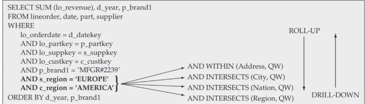
Queries of types 1 to 3 (Section 3) were based on query Q2.3 of the SSB, while query type 4 (Section 3) was based on query Q3.3 of SSB. We replaced the underlined conventional predicates with spatial predicates involving ad hoc query windows (QW) (Figures 3, 4, 5 and 6). These quadratic query windows have a correlated distribution with spatial data, and their centroids are random supplier addresses. Their sizes are proportional to the spatial granularity.

The query windows allow for the aggregation of data at different spatial granularity levels, i.e., the application of spatial roll-up and drill-down operations. Figures 3 to 6 show how complete spatial roll-up and drill-down operations are performed. Both operations comprise four query windows of different sizes that share the same centroid.

Regarding query type 1 (i.e., drill-down/roll-up with one query window that verifies the intersection spatial relation-ship), the Address level was evaluated with the containment relationship and its QW covers 0.001% of the extent. City, Nation and Region levels were evaluated with the intersec-tion relaintersec-tionship and their QW cover 0.05, 0.1 and 1% of the extent, respectively. Figure 3 shows the SQL command for this query type. Table 1 shows the average number of distinct spatial objects returned per query type in each granularity level. In GRSSB, these average numbers are higher.

Address, City, Nation and Region levels of query type 2 (i.e., drill-down/roll-up with one query window that verifies the containment spatial relationship) were evaluated with the containment relationship and their QW covers 0.01, 0.1, 10 and 25% of the extent, respectively. Compared to query type 1, we enlarged the length of the QW for query type 2, aiming at ensuring the recovery of spatial objects for the containment relationship. Figure 4 shows the SQL command for this query type.

Supplier s_suppkey s_address s_address_geo s_city s_city_geo s_nation s_nation_geo s_region s_region_geo ... Date d_datakey d_year ... lineorder lo_orderkey lo_linenumber lo_custkey lo_partkey lo_suppkey lo_orderdate lo_commitdate lo_revenue ... Customer c_custkey c_address c_address_geo c_city c_city_geo c_nation c_region c_region_geo c_nation_geo ... p_partkey p_brand1 ... Part c_custkey c_address c_address_fk c_city c_city_fk c_nation c_region c_region_fk c_nation_fk ... s_suppkey s_address s_address_fk s_city s_city_fk s_nation s_region s_region_fk s_nation_fk ... p_partkey p_brand1 ... Part c_address_pk c_address_geo ... c_address s_address_pk s_address_geo ... s_address d_datekey d_year ... Date city_pk city_geo ... City nation_pk nation_geo ... Nation region_pk region_geo ... Region lineorder lo_orderkey lo_linenumber lo_custkey lo_partkey lo_suppkey lo_orderdate lo_commitdate lo_revenue ...

Customer Supplier

Figure 1. Adapted SSB with spatial data redundancy: GRSSB.

Figure 2. Adapted SSB without spatial data redundancy: GHSSB.

Table 1. Average number of distinct spatial objects returned per

query type.

Query Address City Nation Region

Type 1 22.2 5.6 1.6 1.2 Type 2 190.4 1.4 1.4 0.4 Type 3 1.0 0.8 0.8 1.0

(6)

-As for query type 3 (i.e., drill-down/roll-up with one query window that verifies the enclosure spatial relationship), the Address level was evaluated with the containment rela-tionship, and City, Nation and Region levels were evaluated with the enclosure relationship. Their QW covers 0.00001, 0.0005, 0.001 and 0.01% of the extent, respectively. Compared to query type 1, we reduced the length of the QW for query type 3 in order to ensure the recovery of spatial objects for the enclosure relationship. Figure 5 shows the SQL command for this query type

Finally, query type 4 (drill-down/roll-up with two query windows that verify the intersection spatial relationship) possesses the same characteristics as query type 1. However, this query adds an extra high join cost to process the two spatial query windows. Figure 6 shows the SQL command for query type 4 and Figure 7 depicts the two query windows.

Further details about data and query distribution can be obtained at http://gbd.dc.ufscar.br/papers/jbcs09/figures. pdf.

5. Performance Results and Evaluation

Applied to the GDW Schemas

In this section, we discuss the performance results of two test configurations based on the GRSSB and GHSSB schemas. These configurations reflect current available DBMS resources for GDW query processing, and are described as follows:

•฀ C1:฀star-join฀computation฀aided฀by฀R-tree฀index10_on

spatial attributes.

•฀ C2:฀ star-join฀ computation฀ aided฀ by฀ GiST฀ index8_on

spatial attributes.

Experiments were performed by submitting 5 complete roll-up operations to GRSSB and GHSSB and by taking the average of the measurements for each granularity level. The performance results were gathered based on the elapsed time in seconds.

Sections 5.1 to 5.4 discuss performance results for query types 1, 2, 3 and 4, respectively.

SELECT SUM (lo_revenue), d_year, p_brand1 FROM lineorder, date, part, supplier WHERE

lo_orderdate = d_datekey AND lo_partkey = p_partkey AND lo_suppkey = s_suppkey AND p_brand1 = ‘MFGR#2239’ AND s_region = ‘EUROPE’ GROUP BY d_year, p_brand1 ORDER BY d_year, p_brand1

AND WITHIN (Address, QW) AND INTERSECTS (City, QW) AND INTERSECTS (Nation, QW) AND INTERSECTS (Region, QW)

ROLL-UP

DRILL-DOWN

Figure 3. Adaption of SSB Q2.3 query for query type 1.

AND WITHIN (Address, QW) AND WITHIN (City, QW) AND WITHIN (Nation, QW) AND WITHIN (Region, QW)

ROLL-UP

DRILL-DOWN

AND WITHIN (Address, QW) AND CONTAINS (City, QW) AND CONTAINS (Nation, QW) AND CONTAINS (Region, QW)

ROLL-UP

DRILL-DOWN

(7)

5.1. Results for query type 1

Table 2 shows the results of the performance in processing query type 1, according to the various levels of granularity.

Fidalgo et al.6_{foresaw that although a hybrid GDW}

schema introduces new join costs, it should require less storage space than a redundant one. Our quantitative experi-ments confirmed this fact and also showed that SOLAP query processing is negatively affected by spatial data redundancy in a GDW. According to our results, the attribute granularity does not affect query processing in GHSSB. For instance, Region-level queries took 2787.83 seconds in C1, while Address-Region-level queries took 2866.51 seconds for the same configuration, a very small increase of 2.82%. Therefore, our experiments showed that star-join is the most costly process in GHSSB.

On the other hand, as the granularity level increases, the time required to process a query in GRSSB becomes longer. For example, in C2, a query on the finest granularity level (Address) took 2831.23 seconds, while on the highest granularity level (Region) it took 6200.44 seconds, i.e., an increase of 119%, despite the existence of efficient indices in spatial attributes. Therefore, it can be concluded that spatial data redundancy from GRSSB caused greater performance losses in SOLAP query processing than the losses caused by additional joins in GHSSB.

5.2. Results for query type 2

Table 3 shows the performance results for query type 2, as a function of the various granularity levels. No signifi-cant difference was identified between the use of GiST and R-tree in our experimental work. Nevertheless, our results indicated that the GiST approach may be the better choice in most cases. For this reason, unlikely Table 2, Table 3 lists only the results for configuration C2 and only this configu-ration is taken into account in the remaining sections of this paper.

ROLL-UP

DRILL-DOWN SELECT SUM (lo_revenue), d_year, p_brand1

FROM lineorder, date, part, supplier WHERE

lo_orderdate = d_datekey AND lo_partkey = p_partkey AND lo_suppkey = s_suppkey

AND p_brand1 = ‘MFGR#2239’ AND s_region = ‘EUROPE’ AND c_region = ‘AMERICA’ ORDER BY d_year, p_brand1

AND WITHIN (Address, QW) AND INTERSECTS (City, QW) AND INTERSECTS (Nation, QW) AND INTERSECTS (Region, QW)

}

AND lo_custkey = c_custkey

1 2

City

Nation

Region

Figure 7. Query Windows 1 and 2 for query type 4.

Table 2. Performance obtained with configurations C1 and C2 (query

type 1; elapsed time in seconds)

C1 C2

GRSSB GHSSB GRSSB GHSSB

Address 2854.17 2866.51 2831.23 2853.85

City 2773.39 2763.17 2773.10 2758.70

Nation 4047.35 2766.14 3449.76 2765.61

(8)

For the containment spatial predicate, the performance results were very similar in both GRSSB and GHSSB schemas for the Address and City granularity levels. At these levels, spatial data redundancy does not impair the performance of SOLAP queries. In fact, the Address level has spatial data that are points, which are less costly for calculating spatial relationships. Moreover, addresses are not repeated in the dimension table. Cities are polygons and have a lower degree of spatial data redundancy than the Region and Nation gran-ularity levels in GRSSB schema.

On the other hand, for the granularities levels of Nation and Region, which have a high degree of spatial data redun-dancy in GRSSB schema, the impact of spatial data redunredun-dancy was very high. At the granularity level of Nation, the query processing on the GHSSB schema took 1687.82 seconds, while on the GRSSB schema it took 4026.63 seconds, an increase of 138.56%. At the granularity level of Region, there was an even greater increase of 815.96% due to spatial data redundancy.

Furthermore, the decrease in elapsed time in the SOLAP query processing in GHSSB schema as the granularity level increases reflects the smaller number of answers. For instance, there are far more addresses inside the query windows on the Address level than regions inside the query windows on the Region granularity level.

5.3. Results for query type 3

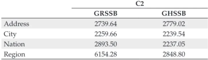
Table 4 lists the performance results for query type 3, as a function of the various granularity levels.

Similarly to the containment spatial predicate, the perform-ance results for the enclosure spatial predicate were very similar in both GRSSB and GHSSB schemas for the Address and City granularity levels. The differences in performance, albeit minor, occurred on the Nation level, i.e., an increase of 29.34%. The performance gap drastically increased at Region level, 116.03%, mainly because this level has a high degree of spatial data redundancy. Furthermore, fewer objects satisfy the enclosure spatial predicate at this level.

5.4. Results for query type 4

Query type 4 is a highly costly SOLAP query that has two spatial query windows. This indicates the need for addi-tional join costs. Due to this overhead, this section discusses performance results specifically to the City granularity level (Table 5). Also, the hardware was upgraded as follows: 7200 RPM SATA 750 GB hard disk with 32 MB of cache, and 8 GB of main memory. For the Region and Nation granularity levels, we aborted SOLAP query processing in GRSSB after 4 days of execution, since this elapsed time is prohibitive.

Even at a level with low degree of spatial data redun-dancy, such as the City granularity level, the performance results clearly indicate that spatial data redundancy drasti-cally impairs the performance of SOLAP queries. While in GHSSB the SOLAP queries took only 130 seconds, in GRSSB the SOLAP queries took 172,900.15 seconds (approximately 48 hours). The increase in the elapsed time was impressive (132.900%).

5.5. Query processing remarks

Although our tests indicate that SOLAP query processing in GHSSB is more efficient than in GRSSB, they also show that both schemas involve prohibitive query response times. Clearly, the challenge in GDW is to retrieve data related to

ad hoc query windows and to avoid the high cost of star-joins. Thus, mechanisms to provide efficient query processing, such as index structures, are essential.

In the next sections, we describe existing indices and offer a brief description of a novel index structure for GDW called the SB-index 29_{. We also discuss how spatial data redundancy}

affects indexing.

6. Indices

In the previous section, we identified reasons for using an index structure to improve SOLAP query performance over GDW. Section 6.1 discusses existing indices for DW and GDW, while Section 6.2 describes our SB-index approach.

6.1. Indices for DW and GDW

The Projection Index and the Bitmap Index are proven valuable choices in conventional DW indexing, since multi-dimensionality is not an obstacle to them20, 31, 35, 36_.

Consider X as an attribute of a relation R. Then, the Projection Index on X is a sequence of values for X extracted from R and sorted by the row number. Undoubtedly, repeated values exist. The basic Bitmap index associates one bit-vector to each distinct value v of the indexed attribute X17_{. The}

bit-vectors maintain as many bits as the number of records

Table 3. Performance results for configuration C2 (query type 2;

elapsed time in seconds).

C2

GRSSB GHSSB

Address 2811.08 3004.44 City 2789.53 2758.30 Nation 4026.63 1687.82 Region 10442.73 1140.09

C2

GRSSB GHSSB

Address 2739.64 2779.02 City 2259.66 2239.54 Nation 2893.50 2237.05 Region 6154.28 2848.80

C2

GRSSB GHSSB

(9)

found in the data set. If X = v for the k-th record of the data set, then the k-th bit of the bit-vector associated with v has the value 1. The attribute cardinality, |X|, is the number of distinct values of X and determines the number of bit-vec-tors. A star-join Bitmap index can be created for the attribute C of a dimension table to indicate the set of rows in the fact table to be joined with a certain value of C.

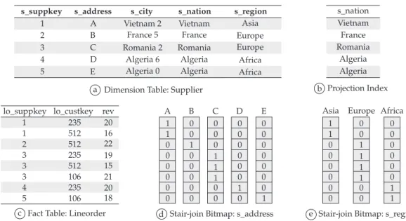
Figure 8 shows data from a DW star-schema (Figures 8a,c), a projection index (Figure 8b) and bit-vectors of two star-join Bitmap indices for attributes s_address and s_region (Figures 8d,e). The attribute s_suppkey is referenced by lo_suppkey shown in the fact table. Although s_address is not involved in the star join, it is possible to index this attribute by a star-join Bitmap index, since there is a 1:1 relationship between s_suppkey and s_address.

Q1 Q2 if, and only if, Q1 can be answered using solely the

results of Q2, and Q1≠ Q2

11_{. Therefore, it is possible to index}

s_region because s_region  s_nation  s_city  s_address. For instance, executing a bitwise OR with the bit-vectors for s_address = ‘B’ and s_address = ‘C’ results in the bit-vector for s_region = ‘EUROPE’. Clearly, creating star-join Bitmap indices to attribute hierarchies suffices to allow roll-up and drill-down operations.

Figure 8e also indicates that rather than storing the value ‘EUROPE’ twice, the Bitmap Index associates this value to a bit-vector and uses 4 bits to indicate the four tuples where s_region = ‘EUROPE’. This simple example shows how Bitmap deals with data redundancy. Furthermore, if a query asking for s_region = ‘EUROPE’ and lo_custkey = 235 were submitted for execution, then a bit-wise AND operation would be executed using the corresponding bit-vectors in order to answer this query. This property explains why the number of dimension tables does not drastically affect the Bitmap efficiency.

High cardinality has been considered the Bitmap’s main drawback. However, recent studies have demonstrated that, even with very high cardinality, the Bitmap index approach can provide an acceptable response time and storage utili-zation36_{. Three techniques have been proposed to reduce the}

Bitmap index size31_{: compression, binning and encoding. The}

FastBit is a Free Software that efficiently implements Bitmap indices with encoding, binning and compression19, 35_{. The}

FastBit creates a Projection Index and an index file for each attribute. The index file stores an array of distinct values in ascending order, whose entries point to bit-vectors.

Albeit suitable for conventional DW, to the best of our knowledge, the Bitmap approach has never been applied to GDW, nor does it the FastBit have resources to support GDW indexing. In fact, only one GDW index has so far been found in the database literature, namely the aR-Tree21_.

The aR-tree index uses the R-tree’s partitioning method to create implicit ad hoc hierarchies for spatial objects. Nevertheless, this is not the case of some GDW applications, which use mainly predefined attribute hierarchies such as region  nation  city  address. Thus, there is a need for an efficient index for GDW to support predefined spatial attribute hierarchies and to deal with multidimensionality.

6.2. The SB-index

The purpose of the Spatial Bitmap Index (SB-index) is to introduce the Bitmap index in GDW in order to reuse this method’s legacy for DW and inherit all of its advantages. The SB-index computes the spatial predicate and transforms it into a conventional one, which can be computed together with other conventional predicates. This strategy provides the whole query answer using a star-join Bitmap index. Thus, the GDW star-join operation is avoided and predefined spatial attributes hierarchies can be indexed. The SB-index therefore provides a means for processing SOLAP operations.

Figure 8. Fragment of data, Projection and Bitmap indices. a) Dimension Table: Supplier; b) Projection Index; c) Fact Table: Lineorder; d)

Star-join Bitmap: s_address; and e) Star-Star-join Bitmap: s_region.

Asia Europe Europe Africa Africa

s_suppkey s_address s_city s_nation s_region

1 A

B C D E 2

3 4 5

Vietnam 2 Vietnam France 5 France Romania 2 Romania

Algeria 6 Algeria Algeria 0 Algeria

s_nation Vietnam France Romania

Algeria Algeria

Projection Index

512 235

235 512

512 106 235 106

1 20

16 22 19 15 21 20 18 1

2 3 3 3 4 5

lo_suppkey lo_custkey rev

Fact Table: Lineorder

A B C D E 1 0 0 0 0 1 0 0 0 0 0 1 0 0 0

1 1 1

1 1

0 0 0 0

Stair-join Bitmap: s_address

1 0 0

0 0 1

1 1 1

1 1

0 0

0 0 0 0

Asia Europe Africa

Stair-join Bitmap: s_region Dimension Table: Supplier

a b

(10)

We have designed the SB-index as an adapted projection index. Each entry maintains a key value and a minimum bounding rectangle (MBR). The key value references the spatial dimension table’s primary key and also identifies the spatial object represented by the corresponding MBR. A DW often has surrogate keys, so an integer value is an appropriate choice for primary keys. A MBR is implemented as two pairs of coordinates. As a result, the size of the SB-index entry (denoted as s) is given by the expression s = sizeof(int) + 4 × sizeof(double).

The SB-index is an array stored on disk. L is the maximum number of SB-index objects that can be stored on one disk page. Suppose that the size s of an entry is equal to 36 bytes (one integer of 4 bytes and four double precision numbers of 8 bytes each) and that a disk page has 4 KB. Thus, we have L = (4096 DIV 36) = 113 entries. To avoid fragmented entries on different pages, some unused bytes (U) may separate them. In this example, U = 4096 – (113 × 36) = 28 bytes.

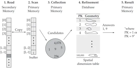
The SB-index query processing illustrated in Figure 9 has been divided into two tasks. The first one performs a sequen-tial scan on the SB-index and adds candidates (possible answers) to a collection. The second task consists of checking which candidates are seen as answers and producing a conventional predicate.

During the scan on the SB-index file, one disk page must be read per step, and its contents copied to a buffer in primary memory. After filling the buffer, a sequential scan on each entry is needed to test the MBR against the spatial predicate. If this test evaluates to true, the corresponding key value must be collected. After scanning the whole file, a collection of candidates is found (i.e., key values whose spatial objects may be answers to the query spatial predicate). Currently, the SB-index supports intersection, containment and enclosure range queries, as well as point and exact queries.

The second task involves checking which candidates can really be considered answers. This is the refinement task

and requires an access to the spatial dimension table using each candidate key value in order to fetch the original spatial object. Clearly, indicating candidates reduces the number of objects that must be queried, and is a good practice to decrease query response time. Then, the previously identified objects are tested against the spatial predicate using proper spatial database functions. If this test evaluates to true, the corre-sponding key value must be used to compose a conventional predicate. Here the SB-index transforms the spatial predicate into a conventional one. Finally, the resulting conventional predicate is given to the FastBit software, which can combine it with other conventional predicates and solve the entire query.

7. Performance Results and Evaluation

Applied to Indices

This section discusses the performance results derived from the following additional test configuration:

•฀ C3:฀SB-index฀to฀avoid฀a฀star-join.

This configuration was applied to the same data and queries used for configurations C1 and C2, in order to compare both C1 and C2 to C3. The experimental setup is the same as that outlined in Section 4.

Our index structure was implemented with C++ and compiled with gcc 4.1. Disk page size was set to 4 KB. Bitmap indices were built with WAH compression35_{and without}

encoding or binning methods.

To investigate the index building costs, we gathered the number of disk accesses, the elapsed time (seconds) and the space required to store the index. To analyze query processing, we collected the elapsed time (seconds) and the number of disk accesses. In the experiments, we submitted 5 complete roll-up operations to schemas GRSSB and GHSSB and took the average of the measurements for each granularity level.

1. Read 2. Scan 3. Collection

Secondary Memory

Primary Memory

4. Refinement 5. Result

Database

Geometry [0]

[1] [2] [3]

[0] [1] [2] [3]

[L-2] [L-1]

[L-2] [L-1] Copy

buffer

Candidates

4,078

1

1 2 3 4

9

256 5

PK

100,000

Spatial dimension table

Answers

1, 9 "where PK = 1 or PK = 9"

(11)

7.1. Results for query type 1

Tables 6 and 7 show the results obtained by applying the building operations of the SB-index to GRSSB and GHSSB, respectively.

Due to spatial data redundancy, all indices in GRSSB have 100,000 entries, and hence, are the same size and require the same number of disk accesses to be built. In addition, the MBR of one spatial object is obtained several times since this object may be found in different tuples, causing an over-head. The star-join Bitmap index occupies 2.3 GB and takes 11,237.70 seconds to be built. Each SB-index requires 3.5 MB, i.e., only a minor addition to storage requirement (0.14% for each granularity level).

Without spatial data redundancy in GHSSB, each spatial object is stored once in each spatial table. Therefore, disk accesses, elapsed time and disk utilization when building the SB-index assume lower values than those mentioned for GRSSB. The star-join Bitmap index occupied 3.4 GB and building it took 12,437.70 seconds. The SB-index adds at most 0.10% to storage requirements, specifically at the Address level. The increase in storage requirements for the SB-index is insignificant at the other three levels.

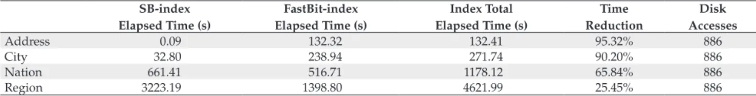
Tables 8 and 9 show the SB-index query processing results for GRSSB and GHSSB, respectively. The time reduction columns in these tables compare how much faster C3 is than the best results of C1 and C2 (Table 2). The SB-index can check if a point (address) lies within a query window without

refine-Table 6. Measurements on building the SB-index for GRSSB.

Elapsed Time (s) Disk Accesses SB-index size

Address 48 886 3.5 MB City 1,856 886 3.5 MB Nation 11,566 886 3.5 MB Region 19,453 886 3.5 MB

Table 7. Measurements on building the SB-index for GHSSB.

Address 18 886 3.5 MB

City 4 4 16 KB

Nation 4 2 8 KB

Region 2 2 8 KB

Table 8. Measurements on query processing with the SB-index for GRSSB (query type 1)

SB-index Elapsed Time (s)

FastBit-index Elapsed Time (s)

Index Total Elapsed Time (s)

Time Reduction

Disk Accesses

Address 0.09 132.32 132.41 95.32% 886

City 32.80 238.94 271.74 90.20% 886

Nation 661.41 516.71 1178.12 65.84% 886

Region 3223.19 1398.80 4621.99 25.45% 886

Table 9. Measurements on query processing with the SB-index for GHSSB (query type 1)

Address 0.09 131.82 131.91 95.38% 886

City 0.07 149.93 150.00 94.56% 4

Nation 0.05 201.65 201.70 92.70% 2

Region 0.05 268.32 268.37 90.38% 2

ment. However, to check if a polygon (city, nation or region) intersects the query window, a refinement task is needed. Thus, the Address level has a greater performance gain.

Query processing using the SB-index in GRSSB performed 886 disk accesses independently of the chosen attribute. This fixed number of disk accesses is due to the fact that we used sequential scan and all indices have the same number of entries for every granularity level (i.e., all indices have the same size).

Redundancy negatively affected the SB-index, since the same MBR may be evaluated several times during both the SB-index sequential scan and the refinement task. On the other hand, adding only 0.14% to storage requirements causes a query response time reduction of 25 to 95%, justi-fying the adoption of the SB-index in GRSSB.

In GHSSB, time reduction was always more than 90%, even better than in GRSSB. This difference is due to the fact that indices had become smaller, because spatial data redun-dancy was avoided. In addition, each MBR is evaluated only once, in contrast to GRSSB. Again, the tiny SB-index requires little storage space and contributes to reduce query response time drastically.

In GRSSB, the overhead of the SB-index was much smaller than that of the FastBit index for Address and City granu-larities. The SB-index took only 0.07% of the elapsed time for Address granularity and 12.07% for the City granularity level. However, as spatial data redundancy increases, the overhead of the SB-index exceeds the overhead of the FastBit index. In Nation granularity, the SB-index took 56.14% of the elapsed time, while in Region granularity the overhead increased and the SB-index took 69.74% of the elapsed time. The increase in the overhead of the SB-index reduces the performance gain (i.e., time reduction column) in SOLAP query performance to 25.45% at the higher granularity level, but is still a substantial improvement.

(12)

7.2. Results for query type 2

The index building costs (i.e., the elapsed time, number of disk accesses and space required to store the index) were the same as those described for query type 1 (Tables 6 and 7). Therefore, similar considerations applied to the intersection spatial predicate are also applied to the containment spatial predicate.

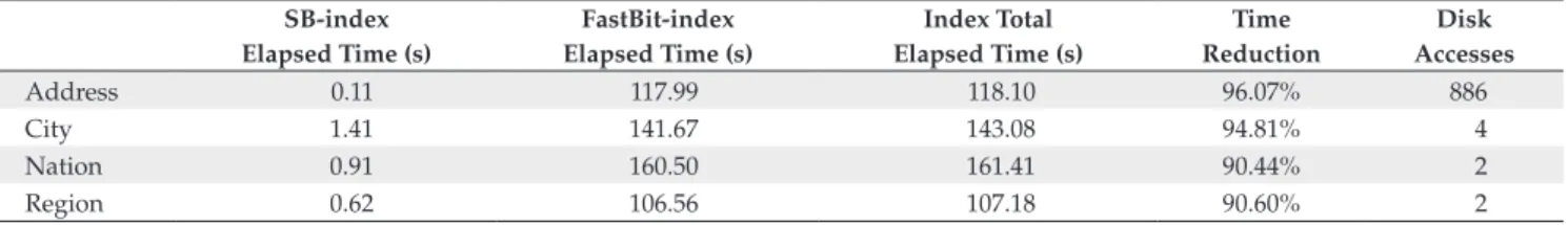
Tables 10 and 11 illustrate the SB-index query processing results for GRSSB and GHSSB, respectively. The time reduc-tion columns in these tables compare how much faster configuration C3 (i.e., which uses the SB-index) is than configuration C2 (star-join with spatial index in Table 3).

The containment spatial predicate is more restricted for polygons than the intersection spatial predicate. Therefore, fewer objects are produced in the set of answers of a SOLAP query. The expected performance gain of the SB-index, there-fore, tends to be higher than the intersection spatial predicate, since fewer objects need to be analyzed in the refinement phase. As observed by4, 1_{, the exact geometry test in the}

refine-ment phase is the most costly part of the spatial processing, since it requires fetching and transferring large objects from disk to the main memory.

In fact, the performance gain of the SB-index was very high for GRSSB, from 78.39 to 94.77%. Unlike the intersec-tion spatial predicate, for the containment spatial predicate the redundancy did not drastically impair the performance gain of the SB-index in GRSSB, although the same MBR may be evaluated several times during the SB-index sequential scan. The SB-index produced even better results for GHSSB, showing a performance gain among 90.44 to 96.07%, similar to the results reported for the intersection spatial predicate.

In GRSSB, the overhead of the SB-index was much smaller than that of the FastBit index for Address and City granulari-ties. The SB-index took only 0.05% of the elapsed time for the Address granularity level and 7.42% for the City granularity level. However, as spatial data redundancy increases, the overhead of the SB-index becomes quite similar or exceeds the overhead of the FastBit index. In Nation granularity, the SB-index took 49.99% of the elapsed time, while in Region

granularity the overhead increased and the SB-index took 68.66% of the elapsed time. The increase in the overhead of the SB-index reduces the performance gain (i.e., time reduc-tion column) in SOLAP query performance. However, this reduction is very small, from 94.77 to 85.61%, and remains a huge improvement.

On the other hand, in GHSSB, the overhead of the SB-index was always much smaller than that of the FastBit index. The SB-index took only 0.09 to 0.99% of the elapsed time, resulting in a considerable time reduction for all granu-larity levels (more than 90%).

7.3. Results for query type 3

The index building costs (i.e., the elapsed time, number of disk accesses and space required to store the index) were the same as those described for query type 1 (Tables 6 and 7). Therefore, similar considerations applied to the intersection spatial predicate are also applied to the enclosure spatial predicate.

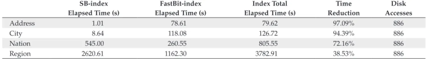
Tables 12 and 13 indicate, respectively, the SB-index query processing results for GRSSB and GHSSB. The time reduction columns in these tables compare how much faster configura-tion C3 (i.e., which uses the SB-index) is than configuraconfigura-tion C2 (star-join with spatial index in Table 4).

The performance gain of the SB-index for GRSSB ranged from very high (97.09%) to significant (almost 40%). Spatial data redundancy impairs the performance gain of the SB-index in GRSSB, particularly because of the huge cost of the refinement phase for complex geometries at the Nation and Region granularity levels. On the other hand, in GHSSB, time reduction always exceeded 90%, which is much better than in GRSSB for the Nation and Region granularity levels. This fact demonstrates the importance of eliminating redun-dancy in a GDW.

In GRSSB, the overhead of the SB-index was much smaller than that of the FastBit index for Address and City granu-larities. The SB-index took only 1.27% of the elapsed time for the Address granularity level and 6.81% for the City

granu-Table 10. Measurements on query processing with the SB-index for GRSSB (query type 2).

Address 0.08 146.96 147.04 94.77% 886

City 12.18 151.96 164.14 94.12% 886

Nation 435.09 435.20 870.29 78.39% 886

Region 1032.06 471.05 1503.11 85.61% 886

Table 11. Measurements on query processing with the SB-index for GHSSB (query type 2).

Address 0.11 117.99 118.10 96.07% 886

City 1.41 141.67 143.08 94.81% 4

Nation 0.91 160.50 161.41 90.44% 2

(13)

larity level. However, as spatial data redundancy increases, the overhead of the SB-index surpasses the overhead of the FastBit index. In Nation granularity, the SB-index took 67.66% of the elapsed time, while in Region granularity the overhead increased slightly and the SB-index took 69.27% of the elapsed time. The increase in the overhead of the SB-index reduces the performance gain (i.e., time reduction column) in SOLAP query performance, but still is a remarkable gain (almost 40%).

On the other hand, in GHSSB, the overhead of the SB-index was always much smaller than the overhead of the FastBit index. The SB-index took only 0.65 to 1.39% of the elapsed time, resulting in a large time reduction for all granu-larity levels (more than 90%).

7.4. Results for query type 4

This section focuses on the query processing according to the City granularity level. Tables 14 and 15 illustrate, respec-tively, the SB-index query processing results for GRSSB and GHSSB. The time reduction columns in these tables compare how much faster configuration C3 (i.e., which uses the SB-index) is than configuration C2 (i.e., star-join with spatial index in Table 5).

The performance gain of the SB-index was very high for GRSSB (99.82%) and GHSSB (76.69%). Therefore, the use of indices showed extremely effective and greatly improved SOLAP query performance. Spatial data redundancy drasti-cally impairs the performance of configuration C2, leading to a prohibitive query performance in GRSSB and an even greater elapsed time in GHSSB (Table 5).

On the other hand, configuration C3 produced an accept-able query performance. Query processing on the GRSSB schema took only few minutes, while on the GHSSB schema it took few seconds. Furthermore, the overhead of the SB-index was much smaller than of the FastBit in both GRSSB and GHSSB.

8. Additional Test: Scalability of Data

Volume

In this section, we investigate the impact of the increase in data volume on the performance of SOLAP query processing. We submitted queries of type 1 to GHSSB and used different scale factors to build the GDW. The chosen scale factors were 2, 6 and 10, representing increasing data volumes. Data generation for scale factor 10 produced 60 million tuples in the fact table, while for the other scale factors the number of tuples in the fact table was proportional to the scale factor 10 (i.e., 1/5 for scale factor 2 and 3/5 for scale factor 6).

Tables 16 to 19 describe the performance results for the Address, City, Nation and Region granularity levels, respec-tively. The time reduction rows in these tables compare how much faster configuration C3 (i.e., which uses the SB-index) is than configuration C2 (i.e., star-join with spatial index). The increase in data volume did not impair the performance gain of configuration C3. In fact, the performance gain was very high and exceeded 89% at all the granularity levels.

Table 12. Measurements on query processing with the SB-index for GRSSB (query type 3).

Address 1.01 78.61 79.62 97.09% 886

City 8.64 118.08 126.72 94.39% 886

Nation 545.00 260.55 805.55 72.16% 886

Region 2620.61 1162.30 3782.91 38.53% 886

Table 15. Measurements on query processing with the SB-index for

GHSSB (query type 4). SB-index

Elapsed Time (s)

FastBit-index Elapsed Time (s)

Index Total Elapsed Time (s)

City 0.60 29.78 30.38 76.69%

Table 13. Measurements on query processing with the SB-index for GHSSB (query type 3).

Address 1.11 78.65 79.76 97.13% 886

City 1.13 112.88 114.01 94.91% 4

Nation 1.51 124.31 125.82 94.38% 2

Region 1.74 265.90 267.64 90.61% 2

Table 14. Measurements on query processing with the SB-index for

GRSSB (query type 4). SB-index

Elapsed Time (s)

FastBit-index Elapsed Time (s)

Index Total Elapsed Time (s)

(14)

9. Redundancy-Based Enhancement

As discussed in Section 7.1, the reason for carrying out the simple and efficient SB-index modification described in this section is to be able to deal quickly with spatial data redun-dancy. An overhead is caused while querying GRSSB because repeated MBR are evaluated and repeated spatial objects are checked in the refinement phase. On the other hand, single MBR values should eliminate this overhead, as is the case of the GHSSB.

Therefore, in this paper we propose a second level for the SB-index, which consists of assigning a list for each distinct MBR. Each list is stored on disk and has all key values asso-ciated with the assigned distinct MBR. In SOLAP query processing, each distinct MBR must be tested against the spatial predicate. If this comparison evaluates to true, one key value from the corresponding list immediately guides

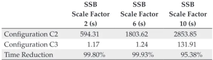
Table 16. Measurements on query processing (query type 1) for GHSSB

using different data volumes at the Address granularity level. SSB

Scale Factor 2 (s)

SSB Scale Factor

6 (s)

10 (s) Configuration C2 594.31 1803.62 2853.85 Configuration C3 1.17 1.24 131.91 Time Reduction 99.80% 99.93% 95.38%

using different data volumes at the Region granularity level. SSB

6 (s)

using different data volumes at the City granularity level. SSB

6 (s)

using different data volumes at the Nation granularity level. SSB

6 (s)

the refinement. If the current spatial object is an answer, then all key values from the list are instantly added to the conven-tional predicate. Finally, the convenconven-tional predicate is passed on to the FastBit, which solves the entire query.

For query type 1, as shown in Tables 6 and 20, the proposed modification of the SB-index drastically decreased the number of disk accesses from 886 to 100 when building the SB-index in GRSSB. The elapsed time to build the SB-index increased slightly at the City granularity level, because of the additional overhead to manipulate the lists of keys applied to a granularity level with low spatial data redundancy. On the other hand, for the Nation and Region granularity levels, which have much more spatial data redundancy, the elapsed time to build the SB-index decreased. The Address granu-larity level was not tested because it is not redundant.

Furthermore, the proposed modification of the SB-index required a very small fraction of the star-join Bitmap index volume, from 0.16 to 0.20%. We conclude that the proposed modification of the SB-index did not impair the performance of the index building operation even for low spatial data redundancy.

In fact, the performance gain resulting from the proposed modification of the SB-index was more effective in the SOLAP query processing. Compared with star-join costs (Tables 2 and 21), the performance gain was very high in GRSSB, varying from 80.41 to 91.74%. Compared with the SB-index without the proposed modification (Tables 8 and 21), the performance gain was also high in GRSSB, ranging from 15.69 to 73.71%.

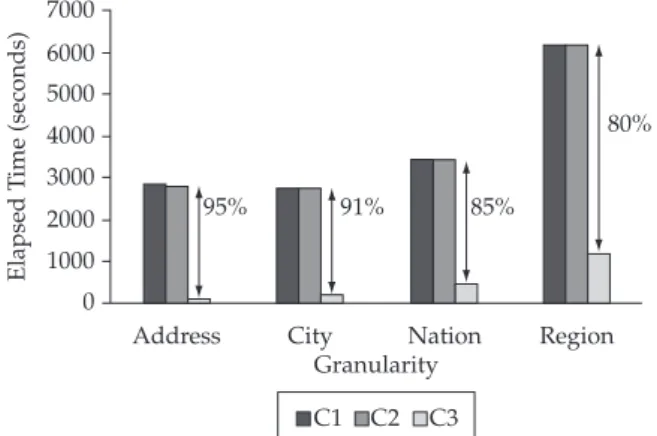
Finally, Figures 10 and 11, respectively, indicate how the SB-index performed in GRSSB and GHSSB, by comparing it to the best results of C1 and C2 (i.e., configurations described in Section 5). The axes indicate the time reduction provided by the SB-index. In Figure 10, except for the Address granu-larity level, the results indicate enhancement of the SB-index’s second level.

Instead of eliminating the redundancy in GDW schemas, we propose a means of reducing its effects. This strategy enhances the SB-index portability, since it allows the SB-index to be used in distinct GDW schemas.

Table 20. Measurements on the enhancement of the SB-index applied

to GRSSB: index building.

City 2,005 100 4.81 MB Nation 11,428 100 3.93 MB Region 19,446 100 3.86 MB

Table 21. Measurements on the enhancement of the SB-index applied

to GRSSB: query processing. Elapsed Time (s)

Star-join