Assessing Reproducibility and Interpretability of
Multivariate fMRI Decoding Models
Bryan R. Conroy*, Jennifer M. Walz, Paul Sajda
Department of Biomedical Engineering, Columbia University, New York, New York, United States of America
Abstract
Multivariate decoding models are increasingly being applied to functional magnetic imaging (fMRI) data to interpret the distributed neural activity in the human brain. These models are typically formulated to optimize an objective function that maximizes decoding accuracy. For decoding models trained on full-brain data, this can result in multiple models that yield the same classification accuracy, though some may be more reproducible than others—i.e. small changes to the training set may result in very different voxels being selected. This issue of reproducibility can be partially controlled by regularizing the decoding model. Regularization, along with the cross-validation used to estimate decoding accuracy, typically requires retraining many (often on the order of thousands) of related decoding models. In this paper we describe an approach that uses a combination of bootstrapping and permutation testing to construct both a measure of cross-validated prediction accuracy and model reproducibility of the learned brain maps. This requires re-training our classification method on many re-sampled versions of the fMRI data. Given the size of fMRI datasets, this is normally a time-consuming process. Our approach leverages an algorithm called fast simultaneous training of generalized linear models (FaSTGLZ) to create a family of classifiers in the space of accuracy vs. reproducibility. The convex hull of this family of classifiers can be used to identify a subset of Pareto optimal classifiers, with a single-optimal classifier selectable based on the relative cost of accuracy vs. reproducibility. We demonstrate our approach using full-brain analysis of elastic-net classifiers trained to discriminate stimulus type in an auditory and visual oddball event-related fMRI design. Our approach and results argue for a computational approach to fMRI decoding models in which the value of the interpretation of the decoding model ultimately depends upon optimizing a joint space of accuracy and reproducibility.
Citation:Conroy BR, Walz JM, Sajda P (2013) Fast Bootstrapping and Permutation Testing for Assessing Reproducibility and Interpretability of Multivariate fMRI Decoding Models. PLoS ONE 8(11): e79271. doi:10.1371/journal.pone.0079271
Editor:Xia Wu, Beijing Normal University, China
ReceivedJune 14, 2013;AcceptedSeptember 27, 2013;PublishedNovember 14, 2013
Copyright:ß2013 Conroy et al. This is an open-access article distributed under the terms of the Creative Commons Attribution License, which permits unrestricted use, distribution, and reproduction in any medium, provided the original author and source are credited.
Funding:This work was supported by National Institutes of Health grant R01-MH085092, the National Science Foundation Graduate Research Fellowship Program, and by the Army Research Laboratories under Cooperative Agreement Number W911NF-10-2-0022. The views and conclusions are those of the authors and should not be interpreted as representing the official policies, either expressed or implied, of the Army Research Laboratory or the U.S. Government. The funders had no role in study design, data collection and analysis, decision to publish, or preparation of the manuscript.
Competing Interests:The authors have declared that no competing interests exist. * E-mail: [email protected]
Introduction
Multivariate pattern analysis (MVPA) is becoming a standard tool for aggregating cortical activity across brain regions to predict various markers of cognitive state related to a task or stimulus condition [1–3]. In contrast to standard univariate statistical tests based on the General Linear Model (GLM) [4], MVPA uses machine learning techniques to extract task-relevant information from spatially-distributed patterns of activity [1,5–14]. As a result, it has the additional benefit of being able to exploit interactions between voxels.
Oftentimes, a related goal of MVPA is to make inferences about the workings of the brain and its underlying cognitive processes. When the machine learning method produces its discriminating component by taking linear combinations of voxels, questions of inference center around interpreting the weights assigned to voxels, which is often called a ‘‘brain map.’’ For this reason, a wave of attention has recently been focused on developing models that are both parsimonious and interpretable. Thus, model
prediction accuracy is not the only goal of the MVPA: the spatial patterns themselves are just as important.
properly statistically assess the thousands of classifiers learned across the brain. By design, this method is also unable to capture interactions between spatially remote regions of the brain.
This paper focuses instead on interpreting brain maps derived from full-brain sparse regression models. In this case, feature selection and dimensionality reduction are not specified a-priori but must be learned, and are thus wrapped into the cross-validation stage of the machine learning procedure. This is usually accomplished in one of two ways. Feature selection techniques [7,17] first perform a univariate selection strategy to identify voxels that are strongly predictive of the brain state of interest. Once the features are identified, a classifier is learned on this reduced data space. Alternatively, a number of groups have applied sparse regression models to full-brain fMRI analysis [13,14], which allows for feature selection and classification to be performed simulta-neously. This is achieved by an objective function that trades off model fit with model complexity. Here, complexity is measured by a regularization term that penalizes a combination of the length (,1-norm) and squared energy (,2-norm) of the regression weights [18,19]. This penalty, called the elastic net, is known to encourage sparse solutions, so that the final predictor is derived from only a small subset of the voxels. Thus, feature selection is performed during the classification procedure. It also leads to a convex optimization problem, which greatly simplifies the optimization procedure. We restrict our attention to the latter method since it is more flexible, but we note that our approach is equally valid for the two-stage feature selection and classification procedure.
We focus on such full-brain classifiers for two reasons. First, they are data-driven and make few assumptions about the location of the brain signal of interest. This allows them to, with minimal prior knowledge, be applied to a wide array of problems and datasets. Second, interpreting brain maps from full-brain analyses is still a challenging problem that lacks a systematic tool for evaluation and interpretation.
Our approach uses a combination of bootstrapping and permutation testing to provide both a measure of cross-validated prediction accuracy and model reproducibility of the learned brain maps. This requires re-training our classification method on many re-sampled versions of the fMRI data. Given the size of fMRI datasets, this is normally a time-consuming process. We, however, make use of our recently proposed FaSTGLZ algorithm [20,21], which was specifically designed to train many related sparse classifiers on a single dataset simultaneously. This makes our approach computationally efficient and feasible.
In conjunction with this approach, we also provide a mechanism to better visualize classification results in two-dimensions: prediction accuracy vs. model reproducibility. This is useful not only as a diagnostic tool to better understand the trade-off between these two possibly competing goals, but it also serves as a means to better inform the model selection stage of analysis. As with most discriminative methods, full-brain classifi-cation models contain regularization parameters that must be tuned [22]. The most common method is cross-validation, in which models are compared based on their predictive power. Given the present discussion, there are obvious limitations in this approach: predictive accuracy addresses how much information is encoded in the brain, but it does not speak to how reproducible and robust the derived spatial patterns are. We consider model selection as a multi-objective optimization problem and provide a principled method to properly take into account both prediction accuracy and model reproducibility. In applying this method to real experimental fMRI datasets, we show empirically that sacrificing a small reduction in cross-validated prediction accuracy generally results in a large and significant improvement in model
reproducibility. This is particularly important when making inferences about activated brain regions that are common to or differ across groups. Furthermore, MVPA provides sufficient sensitivity to identify individual differences within a group, but interpretation of results is robust only when they are reproducible.
Materials and Methods
The data used in this paper are from a previous simultaneous EEG-fMRI experimental study [23]. Only the fMRI data are used in this paper. Details on the behavioral paradigm and data preprocessing are reproduced here for completeness.
Ethics Statement
This study was approved by the Columbia University Institu-tional Review Board and all subjects gave written informed consent in accordance with the guidelines of the Columbia University Institutional Review Board.
Behavioral Paradigm
Fourteen subjects (5 female, mean 27.4 years, range 20–40) participated in three runs each of auditory and visual oddball paradigms. For each oddball detection task, 375 (125 per run) total stimuli were presented for 200 ms each with a 2–3 s uniformly distributed variable inter-trial interval (ITI) and probability of target 0.2. The first two stimuli of each run were constrained to be standards. For the auditory oddball task, the standard stimulus was a 390 Hz pure tone, and the target was a broadband ‘‘laser-gun’’ sound. These were selected based on troughs in the frequency spectrum of the scanner noise, and to match visual discriminator performance of the EEG data. For the visual task, the target and standard stimuli were, respectively, a large red circle and a small green circle on isoluminant gray backgrounds (3.45 and 1.15 visual angles). Subjects were asked to respond to target stimuli only, using a button press with the right index finger on an MR-compatible button response pad. Stimuli were presented to subjects using E-Prime software (PST, Pittsburgh, PA) and a VisuaStim Digital System (Resonance Technology, Northridge, CA), comprised of headphones and 6006800 goggle display.
fMRI Data Acquisition and Preprocessing
A 3T Philips Achieva MRI scanner (Philips Medical Systems, Bothell, WA) was used to collect functional echo-planar image (EPI) data with 3 mm in-plane resolution and 4 mm slice thickness. We covered the entire cortex by obtaining 32 slices of 64664 voxels using a 2000 ms repetition time (TR) and 25 ms
echo time (TE). We also acquired a single-volume high resolution (26262 mm) EPI image and a 16161 mm spoiled gradient recalled (SPGR) image for each subject for purposes of registra-tion.
Using FSL (Smith et al., 2004), we performed bias-field correction on all images to adjust for artifacts caused by the EEG wires. We performed slice-timing correction, motion correction, 0.01-Hz high-pass filtering, and 5-mm full width half max (FWHM) spatial smoothing on the functional data. The structural images were later used to align the functional data to a standard MNI brain.
fMRI Data Processing for MVPA
hemodynamic response function (HRF) evolve over much longer time-scales than the ITI, which results in significant overlap in BOLD response between adjacent trials. To un-mix these overlapping responses, we employed the LS-S deconvolution
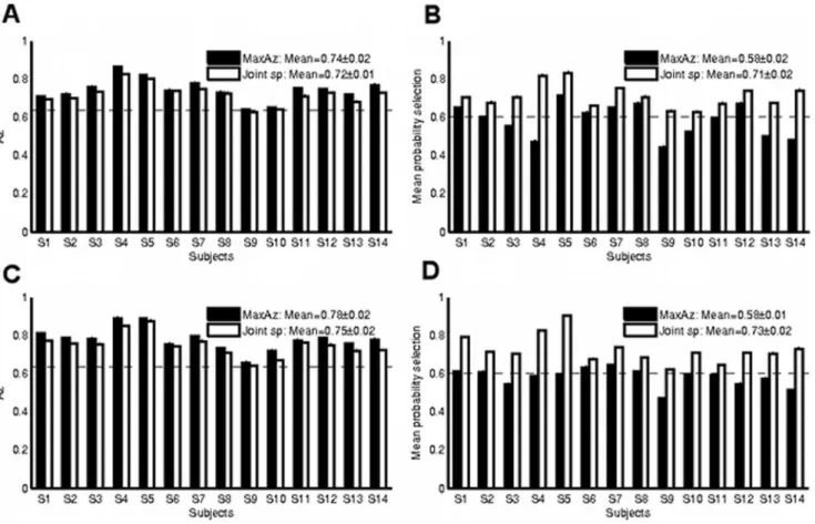
method proposed in [24]. For every trial, the time-series of each voxel is regressed against a ‘‘signal’’ regressor and a ‘‘noise’’ regressor. The ‘‘signal’’ regressor is the modeled HRF response due to that trial (a delta function centered at stimulus onset Figure 1. Comparison of summary statistic results for the MaxAz and Joint sp model selection methods on the auditory oddball data.Dotted horizontal lines indicate the p,0.01 significance levels. Cross-validated prediction accuracy (Az) results for each of 14 subjects under each of the model selection strategies are provided inAfor the without motor network data andCfor the whole brain data. For both model selection methods, prediction accuracy is significant at p,0.01 for all subjects. Reproducibility measure (mean probability of selectionmsp) results for each of 14 subjects under each of the model selection strategies is provided inBfor the without motor network data andDfor the whole brain data. Here, a more drastic difference is noticeable between the two model selection strategies. While the Joint sp method is always above the p,0.01 line, the MaxAz method is significant at p,0.01 for only 7 (without motor network data) and 8 (whole brain data) of the 14 subjects.
doi:10.1371/journal.pone.0079271.g001
Figure 2. Comparison of reproducibility (mean absolute z-scoremDzD) for both model selection methods on the auditory oddball
without motor network data A and auditory oddball whole brain data B.Dotted horizontal lines indicate the p,0.01 significance levels. In both cases, reproducibility increases dramatically under Joint sp for many subjects.
convolved with a canonical HRF), while the ‘‘noise’’ regressor is the modeled HRF response due to all other trials (superimposed linearly). The resulting regression coefficients of the ‘‘signal’’ regressor represent the estimated voxel activations due to that trial. It is important to note that only the trial timing information was used in this step, and not the label information, so there is no need to wrap this preprocessing step into the cross-validation procedure described in the ‘‘Model Selection’’ section below.
Although the exact number of voxels and trials varied for each subject, mean values were n= 36861.2 (s.e.) trials and
p= 51,8046859 (s.e.) voxels. The number of trials varied for each subject because trials missing a button press response were discarded, and trials for which the corresponding EEG data were corrupted were also discarded. Note that classification was performed for each subject in his/her ambient EPI image space (36364 mm). When subsequently comparing across subjects,
brain maps were transformed to the standard MNI brain space using the registrations derived from the structural scan.
Since the task involved a button press only for oddball trials, we expected classifiers derived from the full-brain to be dominated by motor areas. To instead identify regions that are specifically involved in the cognitive task, we additionally performed the classification on the brain data after excluding the ‘‘button press’’ network, which included postcentral and precentral gyrus, thalamus, cerebellum, caudate, putamen, and pallidum. These regions were identified using the MNI152 template brain. Secondary somatosensory cortex was preserved to avoid excluding the neighboring Heschl’s gyrus, which was hypothesized to be important for the auditory oddball task. Overall, this reduced the number of features for this secondary classification analysis to
p= 36,8066653 (s.e.) voxels. To differentiate between the two datasets, we refer to the full analysis as ‘‘whole brain’’, and the secondary analysis as ‘‘without motor network.’’
Figure 3. Reproducibility (msp) vs prediction accuracy (Az) curves for two subjects: A Subject S4 (without motor network), and B
Subject S5 (whole brain).Reproducibility (mDzD) vs prediction accuracy curves for two subjects: C Subject S4 (without motor network), and D Subject
S5 (whole brain). Thick lines indicate the p,0.01 significance thresholds. In each of the figures, the black curve delineates the convex hull of the 1,100 classifiers. Those classifiers that fall in the interior are plotted in gray, while those that lie on the boundary are highlighted. Despite the general trend of a positive correlation between reproducibility and prediction accuracy measures, the MaxAz (red) and Joint sp (magenta) model selection strategies select very different classifiers. In particular, the Joint sp method appears to tradeoff a small reduction in prediction accuracy for a much larger improvement in reproducibility.
Classification Method
Our analysis focuses on the classification problem of predicting the stimulus category (oddball/standard) from the full-brain fMRI data acquired during the experiment. We based our classification model on logistic regression, and treated each voxel as a feature. Thus, our goal is to learn a p-dimensional weight map w on the voxel space that defines a task discriminating ‘‘super-voxel.’’ To avoid overfitting and promote sparse models, we regularized our model by the elastic net penalty [19] so that our objective function may be expressed as:
w~arg min
w ‘(w)zl1k kw 1zl2k kw
2
2 ð1Þ
where ‘(w) is the negative log-likelihood of the logistic regression model. Specifically, given a set of p-dimensional voxel activation maps x1, ,xn for a set of n trials and their associated labelsy1, ,yn (yi= 0 for standards and = 1 for oddballs),‘(w)may be expressed as:
‘(w)~{X n
i~1
yi(xTiw){log(1zexp(xTiw))
Although recent work in function-based registration methods has shown progress in aligning functional areas across subjects [25–28] classifiers were derived independently for each of the 14 subjects to avoid problems of inter-subject variability. In the Results section, we evaluate the inter-subject overlap of areas selected by the classifiers.
Model Selection
For both the auditory and visual oddball tasks, classifiers were trained by 10-fold cross-validation, which was repeated on 10 random partitions. Classifier prediction accuracy was measured by
the area under the ROC curve (Az), averaged over the 10
cross-validation runs.
Typically, model selection involves selecting the classifier with maximal cross-validated prediction accuracy. However, since interpretability of the brain map patterns is also important, we take a similar approach to [29] and consider a balance of prediction accuracy and reproducibility. Although there are many ways to define reproducibility, we focus on a measure of how robustly and reliably the sparse classifier selects voxels. Specifically, letw1, ,wB be a set of p-dimensional brain maps derived by training a classifier on B different training datasets. In this instance, each brain map corresponds to a result trained on one of the cross-validation folds, and B = 100. In general, however, the training sets may also be generated by bootstrap resampling [30]. From the B brain maps, we compute voxel selection probabilities vifor each voxeli~1, ,pas the proportion of times that voxel was included in the model by the classifier. Ideally,viis either 0 or 1 for all voxels, corresponding to perfect voxel selection reliability. As a summary statistic for the classifier, we define the mean selection probability,mspas:
msp~1
A A
X p
i~1
v2i
whereAA is the mean number of voxels selected by the classifier. This statistic may be interpreted as the expected selection probability of a voxel with nonzero weight selected at random from one of the brain maps. Note that sincePpi~1vi~AA, we have thatmspis bounded between 0 and 1, withmsp~1only for perfect voxel selection reliability (vi= 0 or 1 for all voxels).
Model selection is not as straightforward when considering both prediction accuracy (Az) and reproducibility (msp). Unless the two objectives are perfectly correlated, choosing the best classifier
Table 1.Number of significant voxels selected for each of 14 subjects.
Auditory oddball without motor network
#sig (|z|) #sig (sp) A #sig (|z|) #sig (sp) A
S1 44 123 633 S8 3 18 91
S2 23 148 993 S9 0 82 877
S3 51 156 808 S10 0 0 990
S4 125 141 312 S11 29 134 870
S5 46 49 104 S12 71 141 627
S6 12 76 461 S13 18 45 277
S7 117 190 720 S14 24 56 234
Auditory oddball whole brain
#sig (|z|) #sig (sp) A #sig (|z|) #sig (sp) A
S1 25 25 68 S8 21 94 521
S2 74 214 914 S9 2 72 853
S3 72 168 890 S10 7 17 82
S4 317 347 755 S11 18 119 934
S5 59 73 99 S12 61 161 780
S6 24 138 775 S13 19 44 223
S7 90 230 963 S14 43 109 433
#sig (|z|) and#sig (sp) denote the number of voxels deemed significant at FDR = 0.05 when testing z-scores and selection probabilities, respectively. ‘‘A’’ denotes the average number of voxels selected.
entails a tradeoff, which, aside from being dependent on the application, may also be difficult to quantify. In this setting of multiple, possibly competing objectives, selecting a single ‘‘best’’ classifier is not well-defined; however, the set of candidate ‘‘best’’ classifiers are those that are Pareto optimal. These are classifiers that are not dominated by any other classifier, meaning that no other classifier achieves better performance onallof the objectives (reproducibility and prediction accuracy, in this case). For further reference on multi-objective optimization and Pareto optimality, see [31].
Three obvious Pareto optimal points to consider are: (1) the classifier with maximum reproducibility (MaxReprod), (2) the classifier with maximum prediction accuracy (MaxAz), and (3) the classifier that is closest to the optimal point of (reproducibility,-prediction accuracy) = (1,1) (Joint sp)). In this paper, we focus on the latter two classifiers because it allows us to contrast the standard model selection method with a method that takes into account both objectives.
The reproducibility metricmspmeasures how robustly voxels are selected in aggregate, but it does not consider the variability in the weights assigned to these voxels. To take both sources of variability into account, we also consider the mean absolute z-score, mDzD.
Given the w1, ,wB brain maps and corresponding voxel selection probabilities vi, i~1, ,p, let mi and si denote the mean and standard error of the weight for voxel i. A standard score can then be assigned by taking the ratiozi~mi=si. We then definemDzDas:
mDzD~1
A A
X p
i~1 DziDvi
Thus,mDzDis a weighted average of the magnitude of voxel z-scores assigned by the classifier. Analogous to msp above, mDzD may be
interpreted as the expected z-score magnitude of a voxel with nonzero weight selected at random from one of the brain maps. Note that, depending on how the B training sets were derived (e.g., by bootstrap or jackknife sampling), the bootstrap or jackknife estimate of variance can be used to estimate the standard errorssi [30]. SincemDzDis not bounded to a specific range, it is not clear how to scale it in order to produce an appropriate trade-off against the prediction accuracy measure for model selection purposes. Moreover, there is no defined optimal (reproducibility,prediction accuracy) point. For these reasons, we only usemspreproducibility measure when performing joint model selection. However, we show in the results section that, in aggregate,mspandmDzDare very
highly correlated, so thatmspacts as a good surrogate measure.
Results and Discussion
Model Selection: Reproducibility vs. Prediction Accuracy Tradeoff
Classifiers were trained across a set of 1,100 paired values for (l1,l2) using 10-fold cross-validation repeated over 10 random
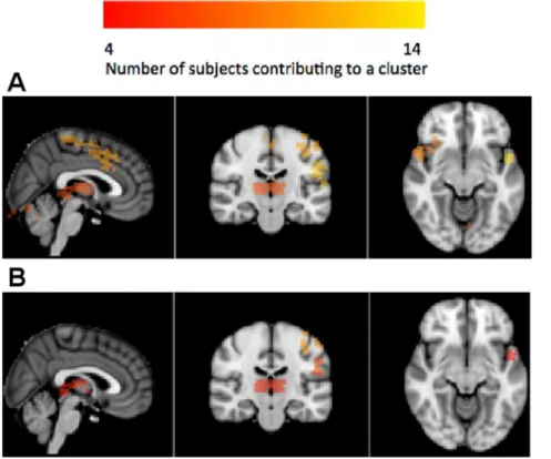
Figure 4. Group-level brain reproducibility maps evaluated on the auditory oddball without motor network data (MNI coordinates: (0,244,28), R-L orientation).Reproducibility was evaluated at the voxel level by testing each voxel’s probability of selection or absolute z-score statistic against a null distribution generated by a permutation test. Subject-specific significance masks were created by thresholding at FDRa= 0.05.
After transforming to MNI space, masks were summed so that the value at each voxel equals the number of subjects that declare it to be significant. This group mask was then spatially clustered and each cluster reports the total number of subjects that contributed to it. (a) Clusters from the selection probability statistic on the without motor network data; (b) Clusters from the absolute z-score statistic on the without motor network data. Associated regions are listed inTable 2.
partitions. Based on previous studies [13] and for memory considerations, we capped the maximum number of voxels to be included by a classifier at 1,000. This resulted in, for each pairing of regularization parameters, 100 brain maps from which to compute reproducibility maps (based on both voxel selection probability and z-scores), and cross-validated prediction accuracy was averaged across the 10 cross-validation runs. Unless stated otherwise, results on the auditory oddball experiment are presented in the main text, while those from the visual oddball experiment are provided in the supplementary material (see
Figure S1, Figure S2, Figure S3, Figure S4andTable S1,
Table S2, Table S3).
To assess statistical significance, we contrasted the results against a permutation test. For each subject, 300 permutations were generated by randomly permuting the response (stimulus category) across trials. The classifier was then re-trained for each permutation along the same set of regularization parameters and cross-validation partitions as the non-permuted case above. For the purposes of generating distributions of summary statistics of prediction accuracy and reproducibility under the null hypothesis of independence between data and response, permutations were pooled across subjects. Thus, to compute the distribution for prediction accuracy, for example, we recorded its maximum value attained over the grid of 1,100 regularization values for each of the 4,200 total permutations. From this distribution, one-tailed significance thresholds were computed (Az= 0.60, p,0.05;
Az= 0.64, p,0.01). This process was repeated for the two
reproducibility measures: (msp= 0.59, p,0.05; msp= 0.60, p,0.01) and (mDzD= 0.37, p,0.05;mDzD= 0.39, p,0.01).
Figure 1 contrasts the summary statistics produced by the
MaxAz and Joint sp model selection methods for each subject on the auditory oddball data. In each of the plots, the dotted horizontal lines indicate the p,0.01 significance thresholds. By definition, the MaxAz classifier will outperform the Joint sp method in terms of prediction accuracy (see Figure 1A and
Figure 1C), but under-perform on the reproducibility (msp) metric
(see Figure 1B and Figure 1D). The more interesting
characteristic of these plots is the degree of difference between the two methods –switching to the joint method incurs a relatively small loss in prediction accuracy in return for a much larger gain in reproducibility. Specifically, prediction accuracy does not fall under the p,0.01 significance line for any of the subjects in either method; in contrast, the joint method is always above p,0.01 in terms of reproducibility (msp), while the MaxAz method is above p,0.01 for only 8 (without motor network) and 7 (whole brain) of the 14 subjects. Moreover, mean (over subjects) prediction accuracy is within the margin of standard error between the two methods, while mean msp is significantly greater under the joint method. Interestingly, the joint method also improves reproduc-ibility in terms of mDzD quite substantially (see Figure 2A and
Figure 2B).
To better visualize this tradeoff,Figure 3plots reproducibility (msp) vs. prediction accuracy (Az) curves for two subjects. Since the
most interesting classifiers lie on the boundary, the figures outline
Figure 5. Group-level brain reproducibility maps evaluated on the auditory oddball whole brain data (MNI coordinates: (2,220,210), R-L orientation).Reproducibility was evaluated at the voxel level by testing each voxel’s probability of selection or absolute z-score statistic against a null distribution generated by a permutation test. Subject-specific significance masks were created by thresholding at FDRa= 0.05.
After transforming to MNI space, masks were summed so that the value at each voxel equals the number of subjects that declare it to be significant. This group mask was then spatially clustered and each cluster reports the total number of subjects that contributed to it. (a) Clusters from the selection probability statistic on the whole brain data; (b) Clusters from the absolute z-score statistic on the whole brain data. The absolute z-score method appears to select a more focal subset. Associated regions are listed inTable 3.
the convex hull of the 1,100 classifiers for each subject as a black curve, and those that lie on this boundary are highlighted. Other classifiers that lie on the interior of the convex hull are plotted in gray. The classifiers corresponding to the MaxAz and Joint sp methods are highlighted in red and magenta, respectively. An interesting characteristic of these plots is that although there is a positive correlation trend between the two objectives, the model selection methods tend to select very different classifiers. Specif-ically, their prediction accuracies are similar but reproducibility scores are much more variable. This suggests that there are a number of models to choose from with competitive prediction accuracies, but widely varying reproducibility scores. Thus, selecting based on prediction accuracy alone is susceptible to marginally improving prediction accuracy at the expense of drastically reducing reproducibility. The joint method appears to overcome this limitation and improve robustness. This is particu-larly true for subjects S4 and S5 (seeFigure 3AandFigure 3B), in which the improvement in reproducibility is most dramatic.
We also assessed the relationship between the two reproduc-ibility measures,msp andmDzD. As outlined in Section 4.3, onlymsp was considered in the model selection stage even thoughmDzD is a
more informative measure of reproducibility. It turns out that both measures are highly correlated, so that one may be used as a surrogate for the other. Across all subjects and datasets, the correlation between the two measures was never less than 0.95.
Figure 3CandFigure 3Dverify that the Joint sp method selects
nearly optimal classifiers when reproducibility is evaluated asmDzD.
Voxel-Based Significance Analysis
The reproducibility measures considered so far provide summaries over the entire brain, but lack specificity on which clusters of voxels in particular are selected by the classifier. In this
section, we assess reliability in terms of the anatomical coordinates of selected voxels. We obtained distributions for voxel-specific selection probabilities and z-scores under the null hypothesis by returning to the permutation analysis described in the previous section. Since there are no spatial priors and voxels are treated equally by the classifier, we assumed that the voxel statistics were identically distributed, which allowed us to pool across voxels. For each permutation, its best classifier was selected using the Joint sp method, and the corresponding z-scores and selection probabilities of any voxels with selection probability vi.0 were used to build the
distributions.
To evaluate voxel-specific significance of a brain map, we first converted the voxel statistics (whether they be z-scores or selection probabilities) of any voxel with vi.0 to p-values based on the null
distributions generated above. We then thresholded the brain map at false discovery rate (FDR) a= 0.05 [32]. Specifically, let p1ƒ ƒpN denote the ordered p-values of the N voxels with nonzero selection probabilities. Then voxels i~1, ,k are deemed significant, where k satisfies:
k~max j:pjƒ j Na
This controls the expected rate of false discoveries ata. This FDR analysis was computed with respect to both voxel selection probabilities and voxel z-scores.
Table 1 lists the number of significant voxels selected by the
selection probability and z-score FDR analysis for both the auditory oddball without motor network and auditory oddball whole brain data. Significant voxels were found for both data except for subjects S9 and S10. Interestingly, these subjects also had the weakest prediction accuracies (see Figure 1A and
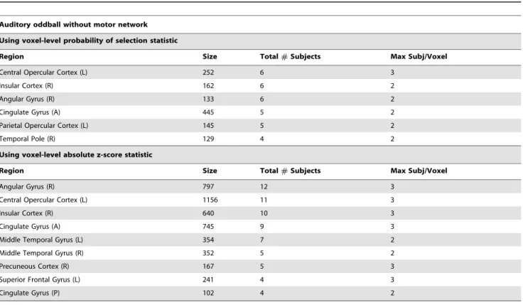
Table 2.Group-level clusters of significant voxels on the auditory oddball without motor network data.
Auditory oddball without motor network
Using voxel-level probability of selection statistic
Region Size Total#Subjects Max Subj/Voxel
Central Opercular Cortex (L) 252 6 3
Insular Cortex (R) 162 6 2
Angular Gyrus (R) 133 6 2
Cingulate Gyrus (A) 445 5 2
Parietal Opercular Cortex (L) 145 5 2
Temporal Pole (R) 129 4 2
Using voxel-level absolute z-score statistic
Region Size Total#Subjects Max Subj/Voxel
Angular Gyrus (R) 797 12 3
Central Opercular Cortex (L) 1156 11 3
Insular Cortex (R) 640 10 3
Cingulate Gyrus (A) 745 9 3
Middle Temporal Gyrus (L) 354 7 2
Middle Temporal Gyrus (R) 352 5 2
Precuneous Cortex (R) 167 5 3
Superior Frontal Gyrus (L) 241 4 3
Cingulate Gyrus (P) 102 4 2
Figure 1C). The selection probability analysis always selects more voxels as significant, and we verified empirically that the voxels selected by the z-score analysis were always a subset of those selected by the selection probability analysis. This suggests a hierarchy of significance testing, in which the selection probabil-ities may be used to identify broad regions that contribute consistently, while the z-scores further refine this to the most reliable and focal regions. In this light, we view both analyses as informative.
To evaluate the regional location and inter-subject spatial overlap, we first transformed the FDR-thresholded brain maps of each subject into MNI space and generated subject-specific brain masks of significant voxels. These masks were then summed over subjects so that the value at each voxel equals the number of subjects that declare it to be significant. Since we do not expect inter-subject spatial overlap on a voxel-by-voxel basis, we instead clustered this group mask and reported the number of subjects that contribute to each of the clusters. The cluster atlas labels, sizes, total number of subjects contributing per cluster, and the maximum number of subjects contributing to a given voxel in the cluster are listed inTable 2andTable 3. Note that since the MNI space is at a higher spatial resolution, the sizes of clusters are inflated. Brain map figures are also provided in Figure 4 and
Figure 5.
As expected for the whole brain data, we found large clusters in regions related to the button press, including thalamus, cerebel-lum, and left (contralateral) postcentral gyrus. For both datasets, discriminating activity was found in central opercular cortex, extending to include auditory regions. Insular cortices, anterior cingulate, and angular gyrus were also consistently selected in both
datasets; these areas are commonly associated with the P300 EEG response that is reliably generated in such oddball decision-making tasks [33]. By excluding the motor network, we detected additional discriminative regions that have been linked to auditory target detection in fMRI data, including the posterior cingulate and right middle temporal gyrus [34].
Summary/Conclusion
We have described an approach for leveraging permutation testing and bootstrapping, together with a method for fast simultaneous training of generalized linear models (FaSTGLZ) to construct a large family of classifiers that we subsequently mapped into a utility space. Within this space optimal classifiers can be identified by considering their joint decoding accuracy and reproducibility. As multivariate decoding models become more prevalent in neuroimaging, and as the dimensions these datasets increase, it is ever more important to systematically explore the accuracy/reproducibility tradeoff. Finally, our methods extend to a wide range of applications of decoding models, from basic exploratory data analysis and inference in cognitive neuroscience to brain computer interfaces and neurofeedback systems.
Supporting Information
Figure S1 Comparison of summary statistic results for the MaxAz and Joint sp model selection methods on the
visual oddball without motor network data. Dotted
horizontal lines indicates the p,0.01 significance thresholds. Cross-validated prediction accuracy (Az) results for each of 14 subjects under each of the model selection strategies. For both
Table 3.Group-level clusters of significant voxels on the auditory oddball whole brain data.
Auditory oddball whole brain
Using voxel-level probability of selection statistic
Region Size Total#Subjects Max Subj/Voxel
Central Opercular Cortex (L) 1153 12 3
Postcentral Gyrus (L) 1020 10 3
Cingulate Gyrus (A) 935 10 3
Insular Cortex (R) 695 9 3
Angular Gyrus (R) 410 9 3
Thalamus (R) 1210 7 4
Cerebellum (R) 262 7 2
Middle Temporal Gyrus (L) 122 7 2
Postcentral Gyrus (R) 528 4 2
Cerebellum (R) 311 4 2
Using voxel-level absolute z-score statistic
Region Size Total#Subjects Max Subj/Voxel
Postcentral Gyrus (L) 637 10 2
Postcentral Gyrus (L) 271 7 2
Supramarginal Gyrus (R) 157 6 2
Thalamus (L) 981 5 2
Central Opercular Cortex (L) 120 5 2
Cingulate Gyrus (A) 403 4 2
Temporal Pole (R) 144 4 2
model selection strategies are provided in (a) for the without motor network data and (c) for the whole brain data. For both model selection methods, prediction accuracy is significant at p,0.01 for all subjects. Reproducibility measure (mean probability of selection msp) results for each of 14 subjects under each of the model selection strategies is provided in (b) for the without motor network data and (d) for the whole brain data. Here, a more drastic difference is noticeable between the two model selection strategies. While the Joint sp method is always above the p,0.01 line, the MaxAz method is significant at p,0.01 for only 4 (without motor network data) and 5 (whole brain data) of the 14 subjects.
(TIF)
Figure S2 Comparison of reproducibility (mean
abso-lute z-scoremDzD) for both model selection methods on the
visual oddball without motor network data (a) and visual
oddball whole brain data (b). Dotted horizontal lines
indicates the p,0.01 significance thresholds. In both cases, reproducibility increases dramatically under Joint sp for many subjects.
(TIF)
Figure S3 Group-level brain reproducibility maps eval-uated on the visual oddball without motor network data
(MNI coordinates: (0,18,8), R-L orientation).For each of
14 subjects, reproducibility was evaluated at the voxel level by testing each voxel’s probability of selection or absolute z-score statistic against a null distribution generated by a permutation test. Subject-specific significance masks were then created by thresh-olding at false discovery rate a= 0.05 to correct for multiple comparisons. After transforming to MNI space, masks were summed so that the value at each voxel equals the number of subjects that declare it to be significant. This group mask was then spatially clustered and each cluster reports the total number of subjects that contributed to it. (a) Group-level clusters derived using the selection prob-ability statistic; (b) Group-level clusters derived using the absolute z-score statistic. The absolute z-score method appears to select a more focal subset. Associated regions are listed inTable S2.
(TIF)
Figure S4 Group-level brain reproducibility maps eval-uated on the visual oddball whole brain data (MNI
coordinates: (0,218,18), R-L orientation).For each of 14
subjects, reproducibility was evaluated at the voxel level by testing each voxel’s probability of selection or absolute z-score statistic against a null distribution generated by a permutation test. Subject-specific significance masks were then created by thresh-olding at false discovery rate a= 0.05 to correct for multiple comparisons. After transforming to MNI space, masks were summed so that the value at each voxel equals the number of subjects that declare it to be significant. This group mask was then spatially clustered and each cluster reports the total number of subjects that contributed to it. (a) Group-level clusters derived using the selection probability statistic; (b) Group-level clusters derived using the absolute z-score statistic. The absolute z-score method appears to select a more focal subset. Associated regions are listed in Table S3.
(TIF)
Table S1 Number of significant voxels selected for each
of 14 subjects.#sig (|z|) and#sig (sp) denote the number of
voxels deemed significant at FDR = 0.05 when testing z-scores and selection probabilities, respectively. ‘‘A’’ denotes the average number of voxels selected.
(DOC)
Table S2 Group-level clusters of significant voxels on the auditory oddball without motor network data.
Associated brain map figures are provided in Figure S3. Notation: (L) – left-lateralized, (R) right-lateralized, (A) anterior, (P) posterior.
(DOC)
Table S3 Group-level clusters of significant voxels on
the auditory oddball whole brain data. Associated brain
map figures are provided in Figure S4. Notation: (L) – left-lateralized, (R) right-left-lateralized, (A) anterior, (P) posterior. (DOC)
Author Contributions
Conceived and designed the experiments: BRC JMW PS. Performed the experiments: BRC JMW. Analyzed the data: BRC. Contributed reagents/ materials/analysis tools: JMW. Wrote the paper: BRC JMW PS.
References
1. Haynes JD, Rees G (2006) Decoding mental states from brain activity in humans. Nat Rev Neurosci. pp. 523–534.
2. Norman KA, Polyn SM, Detre GJ, Haxby JV (2006) Beyond mind-reading: multi-voxel pattern analysis of fMRI data. Trends Cogn Sci. pp. 424–430. 3. Haxby JV (2012) Multivariate pattern analysis of fMRI: The early beginnings.
NeuroImage. pp. 852–855.
4. Smith SM, Jenkinson M, Woolrich MW, Beckmann CF, Behrens TEJ, et al. (2004) Advances in functional and structural MR image analysis and implementation as FSL. NeuroImage 23: 208–219.
5. Haxby JV, Gobbini M, Furey M, Ishai A, Schouten J, et al. (2001) Distributed and overlapping representations of faces and objects in ventral temporal cortex. Science. pp. 2425–2430.
6. Cox DD, Savoy RL (2003) Functional magnetic resonance imaging (fMRI) ‘‘brain reading’’: detecting and classifying distributed patterns of fMRI activity in human visual cortex. NeuroImage. pp. 261–270.
7. Mitchell TM, Niculescu RS, Pereira F, Wang X (2004) Learning to decode cognitive states from brain images. Machine Learning. pp. 145–175. 8. Miranda JM, Bokde AL, Born C, Hampel H, Stetter M (2005) Classifying brain
states and determining the discriminating activation patterns: Support Vector Machine on functional MRI data. NeuroImage. pp. 980–995.
9. Kriegeskorte N, Goebel R, Bandettini P (2006) Information-based functional brain mapping. Proc Natl Acad Sci USA. pp. 3863–3868.
10. Haynes JD, Sakai K, Rees G, Gilbert S, Frith C, et al. (2007) Reading hidden intentions in the human brain. Curr Biol. pp. 323–328.
11. DeMartino F, Valente G, Staeren N, Ashburner J, Goebel R, et al. (2008) Combining multivariate voxel selection and support vector machines for mapping and classification of fMRI spatial patterns. NeuroImage. pp. 44–58. 12. Pereira F, Mitchell T, Botvinick M (2009) Machine learning classifiers and
fMRI: a tutorial overview. NeuroImage. pp. S199–209.
13. Carroll MK, Cecchi GA, Rish I, Garg R, Rao AR (2009) Prediction and Interpretation of Distributed Neural Activity with Sparse Models. NeuroImage. pp. 112–122.
14. Ryali S, Supekar K, Abrams DA, Menon V (2010) Sparse logistic regression for whole-brain classification of fMRI data. NeuroImage. pp. 752–764. 15. Etzel JA, Gazzola V, Keysers C (2009) An introduction to anatomical
ROI-based fMRI classification analysis. Brain Research 1282: 114–125.
16. McKeown MJ, Makeig S, Brown GG, Jung T-P, Kindermann SS, et al. (1998) Analysis of fMRI Data by Blind Separation into Independent Spatial Components. Human Brain Mapping 6: 160–188.
17. Guyon I, Elisseeff A (2003) An Introduction to Variable and Feature Selection. Journal of Machine Learning Research. pp. 1157–1182.
18. Tibshirani R (1996) Regression Shrinkage and Selection via the Lasso. Journal of the Royal Statistical Society, Series B. pp. 267–288.
19. Zuo H, Hastie T (2005) Regularization and variable selection via the elastic net. Journal of the Royal Statistical Society Series B. pp. 301–320.
21. Conroy BR, Walz JM, Cheung B, Sajda P (2013) Fast Simultaneous Training of Generalized Linear Models (FaSTGLZ). arXiv:13078430 [csLG].
22. Hastie T, Tibshirani R, Friedman J (2009) The Elements of Statistical Learning: Data Mining, Inference and Prediction.
23. Walz JM, Goldman RI, Muraskin J, Brown TR, Sajda P (2013) Simultaneous EEG-fMRI Reveals a Superposition of Task-Dependent and Default-Mode Networks During a Simple Target Detection Task. NeuroImage (In Press). 24. Mumford JA, Turner BO, Ashby FG, Poldrack RA (2012) Deconvolving BOLD
activation in event-related designs for multivoxel pattern classification analysis. NeuroImage. pp. 2636–2643.
25. Sabuncu MR, Singer BD, Conroy B, Bryan RE, Ramadge PJ, et al. (2009) Function-based Intersubject Alignment of Human Cortical Anatomy. Cerebral Cortex. pp. 130–140.
26. Conroy BR, Singer BD, Haxby JV, Ramadge PJ (2009) fMRI-Based Inter-Subject Cortical Alignment Using Functional Connectivity. In: Bengio Y, Schuurmans D, Lafferty J, Williams CKI, Culotta A, editors. Advances in Neural Information Processing Systems (NIPS 22). pp. 378–386.
27. Haxby JV, Guntupalli JS, Connolly AC, Halchenko YO, Conroy BR, et al. (2011) A common, high-dimensional model of the representational space in human ventral temporal cortex. Neuron. pp. 404–416.
28. Conroy BR, Singer BD, Guntupalli JS, Ramadge PJ, Haxby JV (2013) Inter-subject Alignment of Human Cortical Anatomy using Functional Connectivity. NeuroImage 81: 400–411.
29. Rasmussen PM, Hansen LK, Madsen KH, Churchill NW (2012) Model sparsity and brain pattern interpretation of classification models in neuroimaging. Pattern Recognition. pp. 2085–2100.
30. Efron B, Tibshirani RJ (1993) Introduction to the bootstrap.
31. Deb K (2009) Multi-Objective Optimization Using Evolutionary Algorithms. 32. Benjamini Y, Hochberg Y (1995) Controlling the false discovery rate: a practical
and powerful approach to multiple testing. Journal of the Royal Statistical Society, Series B. pp. 289–300.
33. Linden DEJ (2005) The P300: Where in the brain is it produced and what does it tell us? The Neuroscientist 11: 563–576.