3D Face Compression and Recognition using
Spherical Wavelet Parametrization
Rabab M. Ramadan
College of Computers and Information Technology University of Tabuk
Tabuk, KSA
Rehab F. Abdel-Kader
Electrical Engineering Department Faculty of Engineering, Port-Said UniversityPort-Said, Egypt
Abstract— In this research an innovative fully automated 3D face compression and recognition system is presented. Several novelties are introduced to make the system performance robust and efficient. These novelties include: First, an automatic pose correction and normalization process by using curvature analysis for nose tip detection and iterative closest point (ICP) image registration. Second, the use of spherical based wavelet coefficients for efficient representation of the 3D face. The spherical wavelet transformation is used to decompose the face image into multi-resolution sub images characterizing the underlying functions in a local fashion in both spacial and frequency domains. Two representation features based on spherical wavelet parameterization of the face image were proposed for the 3D face compression and recognition. Principle component analysis (PCA) is used to project to a low resolution sub-band. To evaluate the performance of the proposed approach, experiments were performed on the GAVAB face database. Experimental results show that the spherical wavelet coefficients yield excellent compression capabilities with minimal set of features. Haar wavelet coefficients extracted from the face geometry image was found to generate good recognition results that outperform other methods working on the GAVAB database.
Keywords-3D Face Recognition; Face Compression; Geometry coding; Nose tip detection; Spherical Wavelets.
I. INTRODUCTION
Representing and recognizing objects are two of the key goals of computer vision systems [1-5]. Computing a compact representation of an item is usually an intermediate stage of the vision system, yielding results used by other processes that perform more abstract operations on the data acquired from the objects. Today, the recent development of 3D sensors and sensing techniques stimulated the demand for visualizing and simulating 3D data. The large amount of information involved and the complexity and speed requirements of the processing techniques demand the development of powerful yet efficient data compression techniques to facilitate the storage and transmission of data. The main objective of compression algorithms is to eliminate the redundancy present in the original data and to obtain progressive representations targeting the best trade-off between data size and approximation accuracy [1]. Recently, the interest in 3D face
compression techniques has risen as a foundation stage in many areas with a wide range of potential applications such as identification systems in the army, hospitals, universities, and banks to medical image compression and videophones, …etc.
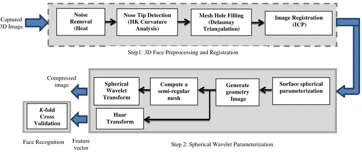
Figure 1: Block diagram of the proposed 3D face compression and recognition system.
In this paper, a robust and accurate 3D face compression and recognition system is proposed. Gaussian curvature analysis is used for nose tip detection and face region extraction. The Iterative closest point (ICP) is employed to automatically align the face image and to perform the required fine pose correction. The system utilizes discriminative spherical wavelet coefficients which are robust to expression and pose variations to efficiently represent the face image with a small set of features. All processes included in the proposed system are fully automated and can be partitioned into two main stages: 3D preprocessing and registration, and spherical wavelet parameterization. The block diagram of the proposed system is presented in Figure 1. Descriptions of each stage are given as follows:
(1) Preprocessing and registration: First we perform image smoothing using heat diffusion to filter out undesirable distortions and noise while preserving important facial features. Second, the nose tip is detected and used to remove irrelevant information such as data corresponding to the shoulder, neck, or hair areas. Third Delaunay Triangulation is applied to fill holes in the mesh of the extracted face region. Finally, the ICP algorithm is used to align the face image and to normalize the effect of face poses and position variations. This registration process typically applies rigid transformations such as translation and rotation on the 3D faces in order to align them.
(2) Spherical wavelet parameterization: Robust feature representation is very important to the whole system. It is expected that these features are invariant to rotation, scale, and illumination. In our systems, we extract compact discriminative features to describe the 3D Faces based on spherical Wavelet coefficients. First, the 3D face is mapped to the spherical parameterization domain. Second, the geometry image is obtained as a color image and a surface image. Third, the spherical based wavelet coefficients are computed for efficient representation of the 3D face. Two different approaches are utilized for obtaining the wavelet coefficients. In the initial approach, the geometry image is transformed to a semi-regular mesh where the spherical wavelet transform is
applied. Alternatively, the Haar wavelet transform can be applied directly to the geometry image.
The rest of this paper is organized as follows: An overview of related work in 3D face compression and recognition is presented in Section II. The preprocessing and normalization tools used in the system are described in Section III. The process of extracting the spherical wavelet coefficients from the 3D face images is explained in Section IV. Section V reports the experimental results and gives some comparisons with existing methods in the literature. Finally, we summarize the paper with some concluding remarks in Section VI.
II. RELATEDWORK
3D meshes are generally used in graphic and simulation applications for approximating 3D Faces. However, Mesh-based surface representations of a face image require large amounts of storage space [1-5]. The emerging demand of applications calling for compact storage, efficient bandwidth utilization, and fast transmission of 3D meshes have inspired the multitude of algorithms developed to efficiently compress these datasets. Image compression has recently been a very active research area but the central concept is straightforward: we transform the image into an appropriate basis and then code only the important expansion coefficients. The problem of finding a good transform has been studied comprehensively from both theoretical and practical standpoints. Excellent survey of the various 3D mesh compression algorithms has been given by Alliez and C. Gotsman in [1, 2]. The recent development in the wavelet transforms theory has spurred new interest in multi-resolution methods, and has provided a more rigorous mathematical framework. Wavelets give the possibility of computing compact representations of functions or data. Additionally, wavelets are computationally attractive and allow variable degrees of resolution to be achieved. All these features make them appear as an interesting tool to be used for efficient representation of 3D objects.
In a typical computer vision system, the compact representation generated from any compression system is used by other processes that perform further operations on the data
Captured 3D Image
Noise Removal
(Heat Diffusion)
Nose Tip Detection (HK Curvature
Analysis)
Mesh Hole Filling (Delaunay Triangulation)
Image Registration (ICP)
Step1: 3D Face Preprocessing and Registration
Step 2: Spherical Wavelet Parameterization
Surface spherical parameterization
K-fold Cross Validation
Generate geometry Image Compute a
semi-regular mesh Spherical
Wavelet Transform
Feature vector
Haar Transform
Compressed image
in the reduced dimension space. Compression algorithms propose a versatile and efficient tool for digital image processing serving numerous applications. 3D Face recognition is one of the imperative applications calling for compact storage and rapid processing of 3D meshes.
Face recognition based on 3D information is not a new topic. It has been extensively addressed in the related literature since the end of the last century [6-11]. Further surveys of the state-of-the-art in 3D face recognition can be found in [7, 8]. Various approaches are reported for extracting and comparing data from facial shapes, each with their own strengths and weaknesses. However, whatever approach is used, three issues always exist that have to be taken into account. (1) The type of facial representation used from which the data is extracted. (2) The way pose or facial orientation differences between different faces are handled which is usually easier in 3D than in 2D but still impose an important challenge. (3) Feature extraction and dimensionality reduction techniques embedded in the system. Several criteria can be adopted to compare existing 3D face algorithms by taking into account the type of problems they address or their intrinsic properties. For example, some approaches perform very well only on faces with neutral expression, whereas other approaches try to address the problem of expression variations. An additional measure of the robustness of the 3D model is its sensitivity to size and pose disparities. This is due to the fact that the distance between the target and the camera can affect the size of the facial surface, as well as its height and depth.
3D Mesh-based surface representation is a popular facial representation strategy used in existing 3D face recognition techniques. In contrast to image-based representations, mesh-based surface representations use a spatially dense discrete sampling across the whole surface, resulting in a 3D point cloud representation of the face. These 3D points can be connected into small polygons resulting in a mesh or wireframe representation of the face. For facial comparison purposes, automated resampling of the facial surface is required to generate consistent and corresponding points. This would be an impossible task manually due to the 1000s of points describing every face. The recognition methods that work directly on 3D point clouds consider the data in their original representation based on spatial and depth information. Point clouds are not properly located on a regular grid therefore a prior registration of the point clouds is usually required. For this purpose, the ICP is the most widely used approach [6]. The classification is generally based on the Hausdorff distance that permits to measure the similarity between different point clouds. Chang et al. [7, 9] register overlapping face regions independently by using an ICP-based multi-region approach. Alternatively, recognition could be performed with “3D Eigen faces” that are constructed directly from the 3D point clouds. Another option is to extract geometrical cues based on Eigen values and singular values of local covariance matrices defined on the neighborhood of each 3D point [7]. The main drawback of the recognition methods based on 3D point clouds however resides in their high computational complexity that is driven by the large size of the data. Spherical representations have been used recently for modeling illumination variations [2, 12-13] or both
illumination and pose variations in face images. Spherical representations permit to efficiently represent facial surfaces and overcome the limitations of other methods towards occlusions and partial views. To the best of our knowledge, the representation of 3D face point clouds as spherical signals for face recognition has however not been investigated yet. We therefore propose to take benefit of the spherical representations in order to build an effective and automatic 3D face recognition system.
III. 3DPREPROCESSING AND REGISTARTION
In this paper, each 3D face is described by a three-dimensional surface mesh representing the visible face surface from the scanner viewpoint. In this section, we describe how the original 3D data are preprocessed. The preprocessing of the 3D face images includes image smoothing and noise removal, nose tip detection, hole filling and the registration of the face surface.
A. Image smoothing
Image smoothing is an essential preprocessing stage that significantly affects the success of any image processing application. The main purpose of image smoothing is to reduce undesirable distortions and noise while preserving important features such as discontinuities, edges, corners and texture. Over the last two decades diffusion-based filters have become a powerful and well-developed tool extensively used for image smoothing and multi-scale image analysis. The formulation of the multi-scale description of images and signals in terms of scale-space filtering was first proposed by Witkin [14] and Koenderink [15].Their basic idea was to use convolutions with the Gaussian filter to removes small-scale features, while retaining the more significant ones and to generate fine to coarse resolution image descriptions. The diffusion process (also called heat equation or anisotropic diffusion), is equivalent to evolving the input image under a smoothing partial differential equation using the classical heat equation. Since the diffusion coefficient in the partial differential equation (PDE) smoothing techniques is designed to detect edges [16-17], the noise can be removed without blurring the edges of the image.
sequential row or column raster ordering of the image pixels then the weight can be calculated as follows:
‖ ‖
0 otherwise (1)
Where X(i) and X(j) are the locations of pixels i and j respectively, r is the distance threshold between two neighboring pixels which controls the local connectivity of the graph, and d(i, j) = | ⃗(i) − ⃗⃗⃗(j)| is the difference between the intensities ⃗(i) and ⃗(j) of the two adjacent pixels indexed i and j. The adjacency weight matrix W is then used to compute the Laplacian matrix L as follows:
L(i, j)= T(i,j)-w(i,j) if i=j -w(i,j) if eijE
0 otherwise (2)
Where T(i ,j) is a diagonal matrix computed as follow:
∑ . The spectral decomposition of L=ɅT, where Ʌ=diag(1,2,….., | | Is the diagonal matrix with the eigenvalues ascending order.
| | is the matrix with the corresponding
ordered eigenvectors as columns.
In order to use the diffusion process to smooth a gray-scale image, we inject at each node an amount of heat energy equal to the intensity of the associated pixel. The heat initially injected at each node diffuses through the graph edges as time progresses. The edge weight plays the role of thermal conductivity. According to the edge weights determined from (1), if two pixels belong to the same region, then the associated edge weight is large. As a result heat can flow easily between them. The heat kernel Ht is a | |x| | symmetric matrix for nodes i, j in the graph the resulting heat element is calculated as follows:
∑| |
(3)
And the heat equation on the graph can be characterized by the following differential equation:
(4)
The algorithm can also be understood in terms of Fourier analysis, which is a natural tool for image smoothing. An image R2 normally contains a mixture of different frequency components. The low frequency components are regarded as the actual image content and the high frequency components as the noise. From the signal processing viewpoint, the approach is an extension of the Fourier analysis to images defined in graphs. This is based on the fact that the classical Fourier analysis of continuous signals is equivalent to the decomposition of the signal into a linear combination of the eigenvectors of the graph Laplacian. The eigenvalues of the Laplacian represent the frequencies of the eigenfunctions. As the frequency component (eigenvalue) increases, then the corresponding eigenvector changes more rapidly from vertex to vertex. This idea has been used for surface mesh smoothing in [19]. The image ⃗ defined on the graph G can be decomposed into a linear combination of the eigenvectors of the graph Laplacian L, i.e.
∑| | (5)
To smooth the image using Fourier analysis, the terms associated with the high frequency eigenvectors should be discarded. However, because the Laplacian L is very large even for a small image, it is too computationally expensive to calculate all the terms and the associated eigenvectors in (5). An efficient alternative is to estimate the projection of the image onto the subspace spanned by the low frequency eigenvectors, as is the case with most of the low-pass filters. We wish to pass low frequencies, but attenuate the high frequencies. According to the heat kernel, the function
acts as a transfer function of the filter such that ≈ 1
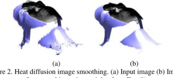
for low frequencies, and ≈ 0 for high frequencies. Therefore, the graph heat kernel can be regarded as a low-pass filter kernel. Figure 2 shows the face image before and after image smoothing.
B. Nose tip detection
Our 3D face compression and recognition system permits the faces to be freely oriented with respect to the camera plane with the only limitation being that no occlusions to hide the major face features such as the eyes, the nose, etc. Having this imperative advantage of being viewpoint invariant requires the detection of some facial features for proper face alignment. In this research alignment was performed automatically in two levels: coarse and fine. The coarse alignment is based on nose tip detection whereas the fine alignment is attained using the ICP registration algorithm. Nose tip is an important face feature point widely used for alignment due to its distinctive features.
(a) (b)
Figure 2. Heat diffusion image smoothing. (a) Input image (b) Image after smoothing using weights from Eq. (1).
The nose is the highest protruding point from the face that is not prone to facial expression. Knowledge of the nose location will enable us to align an unknown 3D face with those in a face database. Besides that, the head pose can be deduced from information obtained from the nose. Therefore nose tip detection is an important part of a 3D face preprocessing [20-25].
using contrast values and edge detection to locate the nose. The drawbacks are SVM has high computational complexity, thus a slow training time while the contrast and edge detection method is affected by expression changes. Using 3D images, one of the methods used was to take horizontal slices of the face and then draw triangles on the slices. The point with the maximum altitude triangle will be considered the nose tip. This method will work for frontal and non-frontal faces. However, for faces tilted to the top, bottom, left or right, errors can occur. This is because in these conditions, the nose tip on the horizontal slices will not be the maximum protruding point. Another method to locate the nose tip from 3D images was proposed by Xu et al. [22]. To locate the nose tip, this method calculates the neighboring effective energy of each pixel to locate suitable nose candidates. It then calculates the neighboring mean and variance of each pixel and then uses SVM to further narrow down the nose tip candidates. Finally, the nose tip is found by choosing the area which has the top three densest nose candidate regions. This method is able to locate nose tip from both frontal and non-frontal faces as well as tilted faces. However, it requires SVM which has high computational complexity.
In this paper the HK curvature analysis is utilized for efficient nose tip detection. To analyze the curvature of 3D faces we let S be the surface defined by a twice differentiable real valued function
f: U R defined on an open set U R2
S= {(x, y, z) (x,y) U, z R; f(x,y) =z} (6) For every point (x, y, z) S we consider two curvature
measures, the mean curvature (H) and the Gaussian curvature (K) defined as follows:
( ) ( )
( ) (7)
( ) (8)
Where fx, fy, fxx, fyy, fxy are the first and second derivatives of f(x, y).
In our system the face image is represented using an NxM range image. Since we have only a discrete representation of S, we must estimate the partial derivatives. For each point (xi,
yj ) on the grid we considered a biquadratic polynomial approximation of the surface:
gij (x, y) = aij + bij (x − xi ) + cij (y − yj ) + dij (x − xi)(y − yj ) +
eij (x − xi )2 + fij (y − yj )2, i= 1 . . . N, j = 1 . . . M (9)
The coefficients aij, bij, cij, dij, eij, fij are calculated by least squares fitting of the points in a neighborhood of (xi, yj ) . The derivatives of f in (xi, yj) are then estimated by the derivatives of gij :
fx(xi, yj ) = bij, fy(xi, yj) = cij, fxy(xi, yj ) = dij , fxx(xi, yj ) = 2eij,
fyy(xi, yj ) = 2fij . (10)
HK classification of the points of the surface is performed to obtain a description of the local behavior of the surface. HK classification was introduced by Besl in 1986 [25]. Image
points can be labeled as belonging to a viewpoint-independent surface shape class type based on the signs of the Gaussian and mean curvatures as shown in Table I.
As proposed by Gordon [26] we use the thresholding process to isolate regions of high curvature and to extract the possible feature points that can be utilized in face alignment during the recognition process. The possible extracted feature points are the two inner corners of the eyes and the tip of the nose. Since the calculation of Gaussian curvature involves the second derivative of the surface function, the noise and the artifacts severely affect the final result and applying a prepressing low-pass filter to smooth the data is required. The surface that either has a peak or a pit shape has a positive Gaussian curvature value (K > 0). Points with low curvature values are discarded: |H(u, v)|Th, |K(u, v)| Tk, where Th and
Tk are predefined thresholds. A nose tip is expected to be a peak (K > TK and H > TH), a pair of eye cavities to be a pair of pit regions (K > TK and H < TH) and the nose bridge to be a saddle region (K < TK and H > TH). These thresholds were experimentally tested to consider a smaller number of cases and reduce the system pipeline overhead, before choosing values similar to those used by Moreno et al. [27] where (Th=0.04; Tk=0.0005).
TABLE I.SURFACE CLASSIFICATION AND THE CORRESPONDING MEAN (H) AND
GAUSSIAN (K) CURVATURES.
K<0 K=0 k>0
H<0
Hyperbolic
Concave( saddle ridge)
Cylindrical
Concave(ridge)
Elliptical
Concave(peak)
H=0
Hyperbolic
symmetric (minimal) Planar(flat) Impossible
H>0
Hyperbolic
Convex (saddle valley)
Cylindrical
Convex (valley)
Elliptical
Convex (pit)
Once the nose tip is successfully determined as the point with maximum z value, we translate it to the origin and align all the face to it. All the points of the face region are located under the nose tip with negative z values. By choosing a proper z- threshold value the face region can be extracted and irrelevant data can be removed such as points corresponding to the hair, neck and shoulders. Figure 3 shows the result of calculating the Gaussian curvature for one of the sample images in the gallery. After localizing the facial area, the portion of the surface below the detected nose tip is projected to a new image to have the face turned upright and where the nose is taken as the origin of the reference system. As can be seen in Figure 3(d) the detected face region contains holes that need to be filled. The Delaunay triangulations algorithm [28] was utilized in this research to fill missing areas in the detected face region and to place them on a regular grid. C. Face Registration
essential to ensure that all 3D face images have the same pose before the spherical parameterization stage. The registration process typically applies rigid transformations on the 3D faces in order to align them. The ICP algorithm (originally Iterative Closest Point, and sometimes known as Iterative Corresponding Point) proposed by Besl and McKay [29] is a well-known standard algorithm for model registration due to its generic nature and its ease of application. ICP has become the dominant technique for geometric alignment of three-dimensional models when an initial estimate of the relative pose is known. Many variants of ICP have been proposed, optimizing the performance of the different stages of the algorithm such as the selection and matching of points, the weighting of the corresponding point pairs, and the error metric and minimization strategies [30-31]. An excellent survey of the recent variants of the ICP algorithm has been given by Rusinkiewicz and Levoy [30].
ICP starts with two point clouds of data X and Y, containing, N points in R3 and an initial guess for their relative rigid-body transform. ICP attempts to iteratively refine the transformation M consisting of a rotation R, and translation T, which minimizes the average distance between corresponding closest pairs of corresponding points on the two meshes. At each ICP iteration, for each point X for i= {1...N}, the closest point, Y is found along with the distance, dN, between the two points.
(a) (b) (c) (d)
Figure 3. HK classification of face image. (a) Mean curvature (b) Gaussian curvature (c) Nose-tip detection (d) Detected face region.
This is the most time consuming part of the algorithm and has to be implemented efficiently. Robustness is increased by only using pairs of points whose distance are below a predefined threshold. As a result of this first step one obtains a point sequence Y = (y1, y2,... ) of closest model face points to the data point sequence X = (x1, x2, …)where each point xi corresponds to the point yiwith the same index. In the second step, the rigid transformation M is computed such that the moved points M(xi) are moved in a least squares sense as close as possible to their closest points on the model shape yi, where the objective function to be minimized is:
∑ ‖ ‖ (11) The singular value decomposition of these points is then
calculated and rotation/ translation parameters are calculated. After this second step the positions of the data points are updated via Xnew = M(Xold). Since the value of the objective function decreases in steps 1 and 2, the ICP algorithm always converges monotonically to a local minimum. This process is repeated either until either the mean square error falls below a predefined threshold or the maximum number of iterations is reached. The generic nature of ICP leads to convergence problems when the initial misalignment of the data sets is large. The impact of this limitation in the ICP process upon
facial registration can be counteracted through the use of preprocessing stage that can be used to give a rough estimate of alignment from which we can be confident of convergence. Generating the initial alignment may be done by a variety of methods, such as tracking scanner position, identification and indexing of surface features, “spin-image” surface signatures, computing principal axes of scans, exhaustive search for corresponding points, or user input. In this paper, we assume that a rough initial alignment is always available through the HK curvature analysis performed in the preceding step. Figure 4 presents the face image before and after the ICP registration process.
IV. SPHERICAL WAVELET PARAMETRIZATION
Wavelets have been a powerful tool in planner image processing since 1985 [1-5, 12, 13, 32-36]. They have been used for various applications such as image compression [1, 2, 5], image enhancement, feature detection [8, 33], and noise removal [32]. Wavelets posse many advantages over other mathematical transforms such as the DFT or DCT as they provide more rigorous mathematical frame work that have the ability of computing accurate and compact representations of functions or data with only a small set of coefficients. Furthermore, wavelets are computationally attractive and they allow variable degrees of detail or resolution to be achieved.
(a) (b)
Figure 4. (a) Face image before registration and fill holes (b) Face image after registration and fill holes.
In the signal processing context the wavelet transform is often referred to as sub-band filtering and the resulting coefficients describe the features of the underlying image in a local fashion in both frequency and space making it an ideal choice for sparse approximations of functions. Locality in space follows from their compact support, while locality in frequency follows from their smoothness (decay towards high frequencies) and vanishing moments (decay towards low frequencies). Therefore, 3D wavelet-based object modeling techniques have appeared recently as an attractive tool in the computer However, traditional 2D wavelet methods cannot be directly extended to 3D computer vision environments, possibly for two main reasons: Wavelet representations are not translation invariant [5, 32]. The sensors used in 3D vision provide data in a way which is difficult to analyze with standard wavelet decompositions. Most 3D sensing techniques provide sparse measurements which are irregularly spread over the object’s external surface. This is also important, because sampling irregularity prevents the straightforward extension of 1D or 2D wavelet techniques.
hierarchical symbolic representations. Wavelets are excellent for creating hierarchical geometric representations, which can be useful in the image data analysis process. Second, going to 3D implies an important increase in complexity. Wavelet decompositions can provide alternative domains in which many operations can be performed effectively. In this paper we utilize a wavelet transform constructed with the lifting scheme for scalar functions defined on the sphere. Aside from being of theoretical interest, a wavelet construction for the sphere has numerous practical applications since many computational problems are naturally stated on the sphere. Examples from computer graphics include: topography and remote sensing imagery, simulation and modeling of bidirectional reflection distribution functions, illumination algorithms, and the modeling and processing of directional information such as environment maps and view spheres. A. Spherical Parameterization
Geometric models are often described by closed, genus-zero surfaces, i.e. deformed spheres. For such models, the sphere is the most natural parameterization domain, since it does not require cutting the surface into disk(s). Hence the parameterization process becomes unconstrained [35]. Even though we may subsequently resample the surface signal onto a piecewise continuous domain, these domain boundaries can be determined more conveniently and a posteriori on the sphere. Spherical parameterization proves to be challenging in practice, for two reasons. First, for the algorithm to be robust it must prevent parametric “foldovers” and thus guarantee a 1 -to-1 spherical map. Second, while all genus-zero surfaces are in essence sphere-shaped, some can be highly deformed, and creating a parameterization that adequately samples all surface regions is difficult. Once a spherical parameterization is obtained, a number of applications can operate directly on the sphere domain, including shape analysis using spherical harmonics, compression using spherical wavelets [2, 5 ], and mesh morphing [36].
Given a triangle mesh M, the problem of spherical parameterization is to form a continuous invertible map φ:
S→M from the unit sphere to the mesh. The map is specified by assigning each mesh vertex v a parameterization φ-1(v) S. Each mesh edge is mapped to a great circle arc, and each mesh triangle is mapped to a spherical triangle bounded by these arcs.To form a continuous parameterization φ, we must define the map within each triangle interior. Let the points {A, B, C} on the sphere be the parameterization of the vertices of a mesh triangle {A'= φ (A), B'= φ (B), C'= φ (C)}. Given a point P'=
αA'+ B'+ C' with barycentric coordinates α+ + =1 within the mesh triangle, we must define its parameterization P =φ -1
(P'). Any such mapping must have distortion since the spherical triangle is not developable.
B. Geometry Image
A simple way to store a mesh is using a compact 2D geometry images. Geometry images was first introduced by Gu et al. [2, 37] where the geometry of a shape is resampled onto a completely regular structure that captures the geometry as a 2D grid of [x, y, z] values. The process involves heuristically cutting open the mesh along an appropriate set of cut paths. The vertices and edges along the cut paths are
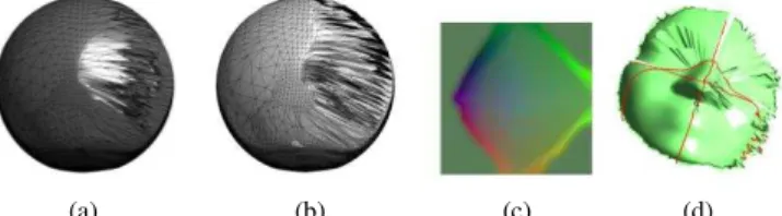
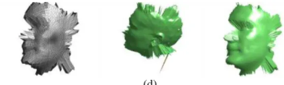
represented redundantly along the boundary of this disk. This allows the unfolding of the mesh onto a disk-like surface and then the cut surface is parameterized onto the square. Other surface attributes, such as normals and colors, are stored as additional 2D grids, sharing the same domain as the geometry, with grid samples in implicit correspondence, eliminating the need to store a parameterization. Also, the boundary parameterization makes both geometry and textures seamless. The simple 2D grid structure of geometry images is ideally suited for many processing operations. For instance, they can be rendered by traversing the grids sequentially, without expensive memory-gather operations (such as vertex index dereferencing or random-access texture filtering). Geometry images also facilitate compression and level-of-detail control. Figure 5(a)-(d) presents the spherical and geometric representations of the face image.
(a) (b) (c) (d) Figure 5. (a) Initial mapping of face mesh on a sphere (b) Final spherical configuration (c) Geometry image as a color image (d) geometry image as a surface image where the red curves represent the seams in the surface to map
it onto a sphere.
C. Wavelet Transform Haar Transform
Geometry images are regularly sampled 2D images that have three channels, encoding geometric information (x, y and z) components of a vertex in R3 [37]. Each channel of the geometry image is treated as a separate image for the wavelet analysis. The Haar wavelet transform has been proven effective for image analysis and feature extraction. It represents a signal by localizing it in both time and frequency domains. The Haar wavelet transform is applied separately on each channel creating four sub bands LL, LH, HL, and HH where each sub band has a size equal to 1/4 of the original image. The LL sub band captures the low frequency components in both vertical and horizontal directions of the original image and represents the local averages of the image. Whereas the LH, HL and HH sub bands capture horizontal, vertical and diagonal edges, respectively. In wavelet decomposition, only the LL sub band is used to recursively produce the next level of decomposition. The biometric signature is computed as the concatenation of the Haar wavelet coefficients that were extracted from the three channels of the geometry image.
Spherical Wavelets
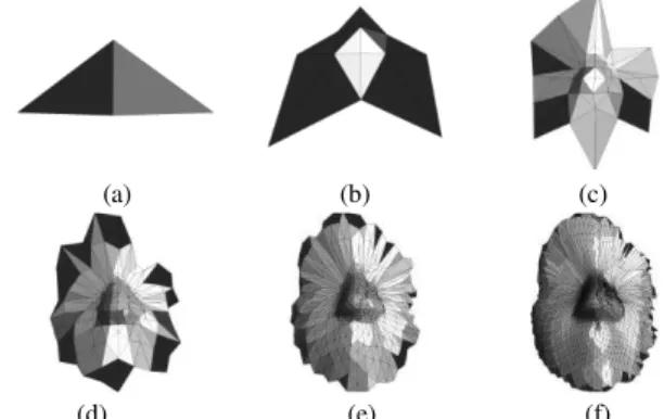
M(j) can be obtained by adding vertices at the midpoint of edges and connecting them with geodesics. Therefore, the complete set of vertices at the j+1th level is given by K(j+1) =K(j) M (j). Consequently, the number of vertices at level j is given by: 10*4j+2. This process is presented in Figure 6 (a)-(f) where the face image is shown at 5 different subdivision levels.
(a) (b) (c)
(d) (e) (f)
Figure 6. Visualization of recursive partitioning of the face mesh at different subdivision levels. (a) Initial icosahedron (scale 0). (b) Single partitioning of icosahedron (scale 1). (c) Two recursive partitioning of icosahedron (scale 2). (d) Three recursive partitioning of icosahedron (scale 3). (e) Four recursive
partitioning of icosahedron (scale 4). (f) five recursive partitioning of icosahedron (scale 5).
In this research, we use the discrete bi-orthogonal spherical wavelets functions defined on a 3-D mesh constructed with the lifting scheme proposed by Schröder and Sweldens [12, 13, 38, 39]. Spherical wavelets belong to second generation wavelets adapted to manifolds with non-regular grids. The main difference with the classical wavelet is that the filter coefficients of second generation wavelets are not the same throughout, but can change locally to reflect the changing nature of the surface and its measure. They maintain the notion that a basis function can be written as a linear combination of basis functions at a finer, more subdivided level. Spherical wavelet basis is composed of functions defined on the sphere that are localized in space and characteristic scales and therefore match a wide range of signal characteristics, from high frequency edges to slowly varying harmonics [38, 40]. The basis is constructed of scaling functions defined at the coarsest scale and wavelet functions defined at subsequent finer scales. If there exist N vertices on the mesh, a total of N basis functions are created, composed of scaling functions and where N0 is the initial number of vertices before the base mesh is subdivided. An interpolating subdivision scheme is used to construct the scaling functions on the standard unit sphere S denoted by j,k. The function is defined at level j and node k k(j) such that the scaling function at level j is a linear combination of the scaling function at level j and j+1. Index j specifies the scale of the function and k is a spatial index that specifies where on the surface the function is centered. Using these scaling functions, the wavelet at level j and node m M(j) can be constructed by the lifting scheme. A usual shape for the scaling function is a hat function defined to be one at its center and to decay linearly to zero. As the j scale increases, the support of the scaling function decreases. A wavelet function is denoted by j,k:S R. The support of the functions becomes smaller as the scale increases. Together, the coarsest level
scaling function and all wavelet scaling functions construct a basis for the function space L2:
{ | } { | } (12)
A given function f: SR can be expressed in the basis as a linear combination of the basis functions and coefficients
∑ ∑ ∑ (13)
Scaling coefficients 0, k represent the low pass content of the signal f, localized where the associated scaling function has support; whereas, wavelet coefficients j,m represent localized band pass content of the signal, where the band pass frequency depends on the scale of the associated wavelet function and the localization depends on the support of the function. Figure 7 (a)-(e) presents the spherical wavelets of the face image.
(a) (b) (c)
(d) (e)
Figure 7. Spherical wavelet transform of face image. (a) using 2% of wavelet coefficients (b) using 5% of wavelet coefficients (c) using 10% of wavelet coefficients (d) using 20% of wavelet coefficients (e) Using all coefficients.
D. Dimensionality Reduction
Principal Component Analysis (PCA) [23] is a well-known technique extensively used for dimensionality reduction in computer vision and image recognition. The basic idea of PCA is to find an alternate set of orthonormal basis vectors which best represent the data set. This is to maintain the information content of the original feature space while projecting into a lower dimensionality space more appropriate for modeling and processing. It is possible to use a subset of the new basis vectors to represent the same data with a minimal reconstruction error.
V. EXPERIMENTAL RESULTS
two frontal views with neutral expression, two x-rotated views (±30º, looking up and looking down respectively) with neutral expression, two y-rotated views (±90º, left and right profiles respectively) with neutral expression and 3 frontal gesture images (laugh, smile and a random gesture chosen by the user, respectively).
A. 3D Face Compression
The spherical wavelet transform can be used to compress the semi-regular mesh by keeping only the biggest coefficients. Different percentages of the biggest wavelet coefficient were examined and each time the inverse wavelet transform was utilized to reconstruct the approximation face. Figure 8 (a)-(e) shows the reconstructed versions of the original face image using different percentages of wavelet coefficients. As can be seen from Figure 8 there is no visually distinguishable difference between the original image and the corresponding reconstructed images using the various subsets of the wavelet coefficients. The face image can be approximated with a reasonable quality using only 2% of the wavelet coefficients. Figure 9 (a)-(d) presents the original mesh, wavelet transform and the reconstructed images for face images with various pose and facial expressions.
(a) (b) (c)
(d) (e)
Figure 8. Wavelet approximation of face image. (a) using 2% of wavelet coefficients (b) using 5% of wavelet coefficients(c) using 10% of wavelet coefficients (d) using 20% of wavelet coefficients (e) Using all
coefficients.
(a)
(b)
(c)
(d)
Figure 9. Wavelet approximation of face image for various facial expressions and orientations. (a) Angry expression (b) Laugh expression
(c) Looking up (d) Looking left.
The Normalized Error (NE) and Normalized Correlation (NC) were used to evaluate the quality of the reconstructed face image. NE is given as follows:
NE= ‖ ‖
‖ ‖ (14)
Where X is the original image and Y is the reconstructed image. i.e. NE is the norm of the difference between the original and reconstructed signals, divided by the norm of the original signal. The NC is given:
∑ ∑
∑ ∑ (15)
Where MxN is the size of the image. The NE and the NC values of the reconstructed images are presented in Table II for the different wavelet subsets.
TABLE II. NE AND NC FOR VARIOUS WAVELET SUBSETS.
2% 5% 10% 20% 100%
NE 0.67 0.3 0.14 0.06 0
NC 0.9982 0.9997 0.9998 1.0 1.0
The NE and NC values indicate that the reconstructed images are the very similar to the original image. In the case of using only 2% of the wavelets coefficients, the relative error of reconstruction is 0. 67%. The reconstructed signal retains approximately 99.33% of the energy of the original signal.
B. 3D Face Recognition
K-fold cross-validation is a well-known statistical method used to evaluate the performance of a learning algorithm [42]. It outperforms the traditional holdout method that divides the dataset into two fixed non-overlapped subsets: one for training and the other for testing. The major drawback of holdout method is that the results are highly dependent on the choice for the training/test split. Alternatively, in k-fold cross validation the data set is partitioned into k equally or nearly equal subsets. Subsequently, k iterations of the holdout method are performed. In each iteration, one of the k subsets is used as the test set and the other k-1 subsets are put together to form a training set. The average error across all k trials is computed. The main advantage of this method is that it is insensitive to how the data gets divided. Every data point gets to be in a test set exactly once, and gets to be in a training set k-1 times. The variance of the resulting estimate is reduced as k is increased. The main disadvantage of this method is that the k iterations of training are required, which means it takes k times as much computation to make an evaluation.
Table III shows the number of the extracted features and the recognition rates for the different feature extraction methods.
TABLE III. RECOGNITION PERFORMANCE FOR VARIOUS FEATURE EXTRACTION METHODS.
Feature Extraction Method Recognition Rate Number of Features
Spherical Wavelet +PCA 21% 2000/300
Haar (2-level decomposition)+ PCA 28% 3072/50
Haar (3-level decomposition)+ PCA 31% 768/50
Haar (4-level decomposition ) 86% 192
The best average recognition rate of 86% is achieved using the 4-level Haar wavelet decomposition with only 192 features. This is a clear indication that the wavelet features extracted from spherical parameterization are a promising alternative for face recognition. However further research is to be performed to improve the recognition rate.
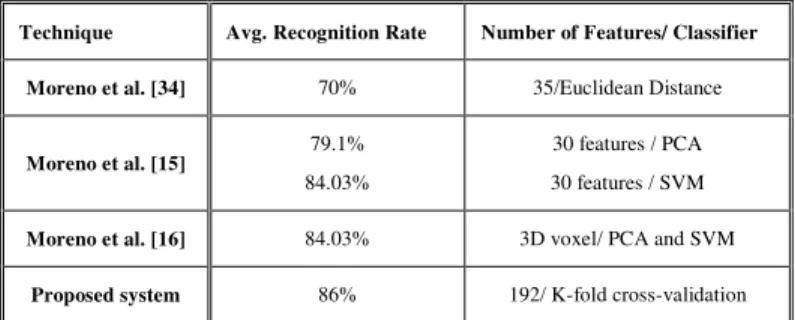
The performance of the proposed face recognition system based upon the 3D face images of the GAVAB dataset was compared to three different approaches presented by Moreno et al. in [43-45]. In the first approach [43], the range images were segmented into isolated sub-regions using the mean and the Gaussian curvatures. Various facial descriptors such as the areas, the distances, the angles, and the average curvature were extracted from each sub-region. A feature set consisting of 35 best features was selected and utilized for face recognition based on the minimum Euclidean distance classifier. An average recognition rate of 70% was achieved for images with neutral expression and for the images with pose and facial expressions. In the second approach [44], a set of 30 features out of the 86 features was selected and an average recognition rates of 79.1% and 84.03%when the images were classified using PCA and support vector machines (SVM) matching schemas respectively. In the third approach [45], the face images were represented using 3D voxels. An average recognition rate of 84.03% was achieved. Table IV
summarizes the results as well as the results obtained from the proposed system.
TABLE IV. COMPARISON OF RECOGNITION RATES FOR VARIOUS 3D FACE RECOGNITION ALGORITHMS BASED ON THE GAVAB DATASET
Technique Avg. Recognition Rate Number of Features/ Classifier
Moreno et al. [34] 70% 35/Euclidean Distance
Moreno et al. [15]
79.1%
84.03%
30 features / PCA
30 features / SVM
Moreno et al. [16] 84.03% 3D voxel/ PCA and SVM
Proposed system 86% 192/ K-fold cross-validation
As shown in Table IV, the proposed method based on 4-level Haar wavelet decomposition yields the best recognition rate of 86%. This is a clear indication that the wavelet feature set extracted from spherical parameterization is a promising alternative for 3D face recognition. However further investigation is to be performed to improve the recognition rate.
VI. CONCLUSION
In this paper an innovative approach for 3D face compression and recognition based on spherical wavelet parameterization was proposed. First, we have introduced a fully automatic process for the preprocessing and the registration of facial information in the 3D space. Next, the spherical wavelet features were extracted which provide a compact descriptive biometric signature. Spherical representation of faces permits effective dimensionality reduction through simultaneous approximations. The dimensionality reduction step preserves the geometry information, which leads to high performance matching in the reduced space. Multiple representation features based on spherical wavelet parameterization of the face image were proposed for the 3D face compression and recognition. The GAVAB database was utilized to test the proposed system. Experimental results show that the spherical wavelet coefficients yield excellent compression capabilities with minimal set of features. Furthermore, it was found that Haar wavelet coefficients extracted from the geometry image of the 3D face yield good recognition results that outperform other methods working on the GAVAB database.
REFERENCES
[1] P. Alliez and C. Gotsman, “Recent advances in compression of 3D
meshes,” In Proceedings of the Symposium on Mult-iresolution in
Geometric Modeling, September 2003.
[2] P. Alliez and C. Gotsman, “Shape compression using spherical geometry
images,” In Proceedings of the Symp. Multi-resolution in Geometric
Modeling, 2003.
[3] J. Rossignac, 3D mesh compression. Chapter in The Visualization Handbook, C. Johnson and C. Hanson, eds., Academic Press, 2003. [4] J. Peng, C.-S. Kim, and C.-C. Jay Kuo, “Technologies for 3D mesh
compression: A survey,” Journal of visual communication and image representation, Vol. 16, pp. 688–733, 2005.
[6] M. H. Mahoora and M. Abdel-Mottalebb, “Face recognition based on 3D
ridge images obtained from range data,” Pattern Recognition, Vol. 42,
pp. 445 – 451, 2009.
[7] K.W. Bowyer, K.Chang, and P. Flynn, “A survey of approaches and
challenges in 3D and multi-modal3D + 2D face recognition,” Computer Vision and Image Understanding, Vol. 101, No.1, pp. 1-15, 2006. [8] A.F. Abate, M. Nappi, D. Riccio and G. Sabatino, “2D and 3D face
recognition: A survey,” Pattern Recognition Letters, Vol. 28, pp. 1885
-1906, 2007.
[9] K. I. Chang, K. W. Bowyer and P. J. Flynn, “Multiple nose region
matching for 3D face recognition under varying facial expression,” IEEE Transactions on Pattern Analysis and Machine Intelligence, Vol. 28, pp. 1695-1700, 2006.
[10] G. Günlü and H. S. Bilge, “Face recognition with discriminating 3D
DCT coefficients,” The Computer Journal, Vol. 53, No. 8, pp. 1324
-1337, 2010.
[11] L. Akarun, B. Gokberk, and A. Salah, “3D face recognition for biometric applications,” In Proceedings of the European Signal Processing Conference, Antalaya, 2005.
[12] P. Schröeder and W. Sweldens, “Spherical wavelets: Efficiently
representing functions on a sphere,” In Proceedings of Computer
Graphics (SIGGRAPH 95), pp. 161-172, 1995.
[13] P. Schröder and W. Sweldens, “Spherical wavelets: Texture processing,”
in Rendering Techniques, New York, 1995, Springer Verlag.
[14] A.Witkin, “Scale-space filtering,” In Proceedings of the International
Joint Conference on Artificial Intelligence, pp. 1019-1021, 1983. [15] J. Koenderink, The structure of images, Biol. Cybern. 50 (1984) pp.
363-370.
[16] G. Sapiro, Geometric partial differential equations and image analysis, Cambridge University Press, Cambridge, 2001.
[17] R. Kondor and J. Lafferty, “Diffusion kernels on graphs and other
discrete structures,” In Proceedings of the 19th International Conference on Machine Learning, pp. 315-322, 2002.
[18] F. Zhang and E. R. Hancock, “Graph spectral image smoothing using the
heat kernel,” Pattern Recognition, Vol. 41, pp. 3328 - 3342, 2008.
[19] G. Taubin, “A signal processing approach to fair surface design,” In
Proceedings of SIGGRAPH, , pp. 351-358, 1995.
[20] A. Colombo, C. Cusano, and R. Schettini, “A 3D face recognition
system using curvature-based detection and holistic multimodal classification,” In Proceedings of the 4th International Symposium on Image and Signal Processing and Analysis , pp. 179-184, 2005.
[21] A. Colombo, C. Cusano, and R. Schettini, “3D face detection using
curvature analysis,” Pattern Recognition, Vol. 39, pp. 444 – 455, 2006.
[22] C. Xu, T. Tan, Y. Wang, and L. Quan, “Combining local features for
robust nose location in 3D facial data," Pattern Recognition Letters, Vol. 27, pp.1487–1494, 2006.
[23] A. Hesher, A. Srivastava, and G. Erlebacher, “Principal component analysis of range images for facial recognition,” In Proceedings of International Conference on Imaging Science, Systems and Technology (CISST 2002).
[24] J. Sergent, “Microgenesis of face perception,” In: H.D. Ellis, M.A.
Jeeves, F. Newcombe and A. Young, Editors, Aspects of Face Processing, Nijhoff, Dordrecht (1986).
[25] P. J. Besl and R.C. Jain, “Invariant surface characteristics for 3-d object
recognition in range images,” Computer Vision, Graphics Image Process. Vol. 33, pp. 33-80, 1986.
[26] G.G. Gordon, “Face recognition based on depth maps and surface
curvature,” SPIE Geom. Methods Computer Vision, Vol.1570,pp. 234
-274, 1991.
[27] A. Moreno, A. Sanchez, J. Velez, and F. Diaz, “Face recognition using
3d surface extracted descriptors,” In Proceedings of the Irish Machine Vision and Image Processing, 2004.
[28] D. Cohen-Steiner and J.-M. Morvan, “Restricted delaunay triangulations and normal cycle,” In Proceedings of the nineteenth annual symposium on Computational geometry, pp. 312-321, 2003.
[29] P. J. Besl and N. D. McKay, “A method for registration of 3D shapes,”
IEEE Trans. Pattern Analysis and Machine Intelligence, Vol. 14, No.2, pp. 239-256, 1992.
[30] S. Rusinkiewicz and M. Levoy, “Efficient variants of the ICP algorithm,” In Proceedings of the. 3rd Int. Conf. on 3D Digital Imaging and Modeling, Quebec, 2001.
[31] J. Cook, V. Chandran, S. Sridharan, and C. Fookes, “Face recognition
from 3D data using iterative closest point algorithm and Gaussian
mixture models,” In Proceedings of the 2nd International Symposium on 3D Data Processing, Visualization, and Transmission, 2004. [32] J. Stollnitz, T. D. DeRose, and D. H. Salesin, Wavelets for computer
graphics: theory and applications. San Francisco, CA: Morgan Kaufmann, 1996.
[33] Q. M. Tieng and W. W. Boles, “Recognition of 2D object contours using
the wavelet transform zero crossing representation,” IEEE Transactions Pattern Analysis and Machine Intelligence, Vol.19, No. 8, pp. 910–916, 1997.
[34] P. Wunsch and A. F. Laine, “Wavelet descriptors for multi resolution
recognition of hand printed characters,” Pattern Recognition, Vol. 28 No. 8, pp. 1237–1249, 1995.
[35] Praun and H. Hoppe, “Spherical parameterization and remeshing,” in
ACM SIGGRAPH 2003, pp. 340–349, 2003.
[36] M. Alexa, “Recent advances in mesh morphing,” Computer Graphics
Forum, Vol. 21, No. 2, pp. 173-196, 2002.
[37] X. Gu, S. J. Gortler and H. Hoppe, “Geometry images,” ACM
SIGGRAPH, pp. 355-361, 2002.
[38] P. Schröeder and W. Sweldens, “Spherical wavelets: efficiently
representing functions on a sphere,” In Proceedings of Computer Graphics (SIGGRAPH 95), pp. 161-172, 1995.
[39] S. Campagna and H.-P. Seidel, Parameterizing meshes with arbitrary topology. In H.Niemann, H.-P. Seidel, and B. Girod, editors, Image and
Multidimensional Signal Processing’ 98, pp. 287-290, 1998.
[40] P. Yu, P. Ellen Grant, Y. Qi, X. Han, F. Ségonne and Rudolph Pienaar, “
Cortical surface shape analysis based on spherical wavelets,” IEEE Transactions on Medical Imaging, Vol. 26, No. 4, pp. 582-597, 2007.
[41] A.B. Moreno and A. Sanchez, “GavabDB: A 3D Face Database,” In
Proceedings of 2nd COST Workshop on Biometrics on the Internet: Fundamentals, pp. 77-82, 2004.
[42] A.Blum, A. Kalai, and J. Langford, “Beating the hold-out: bounds for
K-fold and progressive cross validation,” In Proceedings of the twelfth
annual conference on Computational learning theory, pp. 203-208, 1999.
[43] A.B. Moreno, A. Sanchez, J.F. Velez and F. Dkaz, “Face recognition
using 3d surface- extracted descriptors,” In Proceedings of Irish Machine Vision and Image Processing Conference 2003 (IMVIP'03), 2003.
[44] A.B. Moreno, A. Sanchez, J.F. Velez and F.J. Dkaz, “Face recognition
using 3d local geometrical features: PCA vs. SVM,” In Proceedings of Fourth International Symposium on Image and Signal Processing and Analysis (ISPA 2005), 2005.
[45] A.B. Moreno, A. Sanchez and J.F. Velez, “Voxel-based 3d face
representations for recognition,” in: 12th International Workshop on Systems, Signals and Image Processing (IWSSIP'05), 2005.
AUTHORS PROFILE
Rabab Mostafa Ramadan attended Suez Canal University, Port-Said, Egypt majoring in Computer Engineering, earning the BS degree in 1993. She graduated from Suez Canal University, Port-Said, Egypt with a MS degree in Electrical Engineering in 1999. She joined the Ph.D. program at Suez Canal University, Port-Said, Egypt and earned her Doctor of Philosophy degree in 2004. She worked as an Instructor in the Department of Electric Engineering (Computer division), Faculty of Engineering, Suez Canal University. From 1994 up to1999 , as a lecturer in Department of Electric Engineering (Computer division), Faculty of Engineering , Suez Canal University From 1999 up to 2004, and as an assistant Professor in Department of Electric Engineering(Computer division), Faculty of Engineering , Suez Canal University From 2004 up to 2009. She is currently an Assistant professor in Department of Computer Science, College of Computer & Information Technology, Tabuk University, Tabuk, KSA. Her current research interests include Image Processing, Artificial Intelligence, and Computer Vision.