www.nat-hazards-earth-syst-sci.net/14/675/2014/ doi:10.5194/nhess-14-675-2014
© Author(s) 2014. CC Attribution 3.0 License.
Natural Hazards
and Earth System
Sciences
Landslide observation and volume estimation in central Georgia
based on L-band InSAR
E. Nikolaeva1, T.R. Walter1, M. Shirzaei1,*, and J. Zschau1
1Department 2 – Physics of the Earth, Helmholtz Center Potsdam – GFZ German Research Center of Geosciences, Potsdam, Germany
*now at: School of Earth and Space Exploration, Arizona State University, Tempe, AZ 85287-6004, USA
Correspondence to:E. Nikolaeva ([email protected])
Received: 21 August 2013 – Published in Nat. Hazards Earth Syst. Sci. Discuss.: 17 September 2013 Revised: 9 December 2013 – Accepted: 30 January 2014 – Published: 25 March 2014
Abstract.The republic of Georgia is a mountainous and
tec-tonically active area that is vulnerable to landslides. Because landslides are one of the most devastating natural hazards, their detection and monitoring is of great importance. In this study we report on a previously unknown landslide in cen-tral Georgia near the town of Sachkhere. We used a set of Advanced Land Observation Satellite (ALOS) Phased Array type L-band Synthetic Aperture Radar (PALSAR) data to generate displacement maps using interferometric synthetic aperture radar (InSAR). We detected a sliding zone of di-mensions 2 km north–south by 0.6 km east–west that threat-ens four villages. We estimated surface displacement of up to ∼30 cm/yr over the sliding body in the satellite line-of-sight (LOS) direction, with the largest displacement occurring af-ter a local tectonic earthquake. We mapped the morphology of the landslide mass by aerial photography and field survey-ing. We found a complex set of interacting processes, includ-ing surface fracturinclud-ing, shear and normal faults at both the headwall and the sides of the landslide, local landslide ve-locity changes, earthquake-induced veve-locity peaks, and loss in toe support due to mining activity. Important implications that are applicable elsewhere can be drawn from this study of coupled processes.
We used inverse dislocation modelling to find a possible dislocation plane resembling the landslide basal décollement, and we used that plane to calculate the volume of the land-slide. The results suggest a décollement at∼120 m depth, dipping at∼10◦sub-parallel to the surface, which is indica-tive of a translational-type landslide.
1 Introduction
1.1 Landslides in Georgia
Landslides and related hazards are widespread in Georgia (Nadim et al., 2006; Gracheva and Golyeva, 2010) and cause substantial damage annually (van Westen et al., 2012). The steep hillslopes, active geology and wet or even subtropical climatic conditions in Georgia (van Westen et al., 2012) are important factors that contribute to the high landslide sus-ceptibility there. Over 5700 landslides have been identified, ranging from small-scale slumps to large-scale mass wast-ing of entire hillsides (van Westen et al., 2012). Approxi-mately 700 of those landslides have been identified through year-long mapping and fieldwork activities. A recent land-slide susceptibility analysis based on geology, slope classifi-cation and land cover mapping suggested that approximately 17 % of Georgia is located in high-hazard zones, and another 38 % is located in moderate-hazard zones (van Westen et al., 2012). Landslide concentration is especially high and cov-ers all scales in Adzharia, a region in southwestern Georgia with a humid subtropical climate, with occurrence peaking in spring and during summer storms (Gracheva and Golyeva, 2010).
highlights the importance of monitoring slow-moving land-slides that may accelerate due to unpredictable external trig-gers. Slow-moving landslides in Georgia in particular can ac-celerate abruptly, especially if extrinsic factors act as triggers (Gracheva and Golyeva, 2010).
Although geologic mapping has been performed for some of these landslides, dynamic and kinematic analyses of them have received little scientific attention. As will be shown in this work, space-based data allow analysis of displacement rates and the identification of possible detachment planes of a landslide, which, together with aerial images, provide a de-tailed view of unstable masses and triggering factors ranging from tectonics to man-made activity.
1.2 Landslide mechanisms
The dynamics, i.e. the appearance and displacement pattern of a landslide, is primarily controlled by the geometry of the sliding planes (Cruden, 1986). These planes are made up of a combination of basal décollements and laterally delimit-ing fractures. The décollement is usually not directly visible and is also difficult to infer from remote sensing techniques. Therefore, little is known about the geometric complexities and dynamics of active décollement planes. The laterally de-limiting fractures, in turn, are visible at the surface and com-monly include a headwall fault, which is the surface expres-sion of the main detachment, en echelon sets of strike-slip and normal faults on either side with opposite senses and a compressional zone in the landslide toe that forms thrust and fold belts. The geometry of these sliding planes affects the different types of movement. Movement of a landslide can be translational, rotational, or complex (Cruden and Varnes, 1996). Rotational landslides move generally downward and outward and are thought to be structurally confined by a curved basal detachment plane (Highland and Bobrowsky, 2008). Translational slides move hillslope-parallel and are structurally defined by a planar slope-parallel plane (High-land and Bobrowsky, 2008). Most (High-landslides likely involve a combination of rotational and translational mechanisms. Be-cause the network of these structures delimits the mass of a landslide, structural characterisation of a landslide is impor-tant for assessing the landslide volume.
Landslides exhibit a wide range in velocity, from ex-tremely slow (10 mm year−1) to extremely rapid landslides
(10 m/s) (Cruden and Varnes, 1996). This broad velocity range highlights a common problem in landslide monitor-ing: the ability to detect and explore several scales of dis-placement magnitude. This problem is described further in the following section.
1.3 Landslide detection and displacement monitoring
Most active landslides are studied using field-based mor-phological, structural and kinematic analyses. Ground-based techniques are not appropriate for detecting a landslide in a broad area because of the limited spatial resolution. Non-intrusive remote sensing techniques have therefore become widely used for the detection and mapping of the position, size and shape of landslides (Cardenal et al., 2001; Guzzetti et al., 2012) and potentially unstable slopes (Colesanti and Wasowski, 2006; Ouimet, 2010). Remote sensing techniques have specifically contributed to define states of activity, to monitor landslides, to improve hazard analysis and to al-low implementation in early warning systems (Canuti et al., 2007). Remote sensing methods include aerial photographs, multispectral optical images (Qi et al., 2010), differential digital elevation models (DEMs) (Casson et al., 2005), in-terferometric analysis of radar images (Riedel and Walther, 2008) and lidar data (Schulz 2004; Jaboyedoff et al., 2010) and others.
The most commonly used method for landslide detec-tion is the visual interpretadetec-tion of optical images (Tofani et al., 2013). Change detection techniques (Nichol and Wong, 2005) and classification with semi-automated object-oriented methods (Martha et al., 2010) in optical imagery allow for landslide mapping. Together with detection, these methods allow monitoring and reconstruction of year-long time series. For instance, rapid and large morphometric changes can be quantified using change detection methods applied to high-resolution optical data (Nichol and Wong, 2005). The com-bination of these methods is also used to improve landslide inventory maps (Guzzetti et al., 2012).
Interferometric synthetic aperture radar (InSAR) tech-niques allow mapping of ground movement that occurs be-tween two acquisition times (Hanssen, 2001). InSAR tech-niques are increasing in popularity for landslide applica-tions (Colesanti and Wasowski, 2006; Riedel and Walther, 2008; Tofani et al., 2013) as they are low-cost, almost glob-ally applicable, high-resolution and independent of day or night. The traditional two pass differential InSAR method allows the detection and monitoring of slow (several cm per year) landslides, following the classifications of Cruden and Varnes (1996). Persistent scatterers SAR interferometry (PS-InSAR) and Small BAseline Subset (SBAS) techniques al-low analysis of the temporal and spatial evolution of ex-tremely slow landslides (several mm per year) (Colesanti et al., 2003b; Hilley et al., 2004; Guzzetti et al., 2009). Com-binations of different InSAR techniques are useful to detect and investigate different rates of landslides (García-Davalillo et al., 2013).
Fig. 1.Map of central Georgia showing land cover based on Landsat
TM information. The combination of bands 5, 4 and 3, represented with red, blue and green, respectively, shows vegetation in bright green colours and soil in mauve colours. The violet curves close to Sachkhere and Chiatura show the main path of the Kvirila River. The location of the Itskisi landslide is near Sachkhere. Faults indi-cated by white symbols are thrust faults. The faults were defined by Gamkrelidze (1978).
spectral and, foremost, InSAR data to analyse the dynamics and changes of a landslide.
2 Study area
We concentrate our study on a site located in the central western part of Georgia (42.30◦N, 43.48◦E) because of
the known landslide potential, slope angle and field access there. We use a specific constellation to investigate the ef-fect of extrinsic forcing (Fig. 1). Geologically, the region belongs to the Dzirula block, which is a topographic fea-ture of the Chiatura formation (Gamkrelidze and Shengelia, 2007) (Fig. 1). The geologic Chiatura formation was created by sedimentary deposition, with a sequence of quartz-arkosic sandstones and sands underlying an ore horizon that is over-lain by siliceous sedimentary rocks to the west and shales and shaly sandstones to the east (Edilashvili et al., 1974; Leonov, 1976).
The relief profile of the study area shows a gently slop-ing morphology. The height varies only from 500 to 850 m; thus the slope is moderate, with slope angles less than 20◦.
A significant part of the lower landslide flank is subject to mining activity (Fig. 2), where quartz sand is excavated. The nearby Kutaisi-Sachkhere thrust fault, located just∼5 km to the north of the landslide area (Gamkrelidze and Shengelia, 2007), is thought to be active (seismic catalogue of Geor-gia, http://seismo.ge) and thus has the potential to be an un-predictable landslide trigger (Fig. 1). Other faults at larger distances may also dynamically trigger the landslide,
simi-Fig. 2.Time series of Landsat images showing the development of
the mining area. The spatial resolution of the images is 30 m. These images emphasise the vegetation and the boundary between land and water. Bright colours indicate bare soil, which in this case is the mining area. Panels(d–f)show several expansions that have opened
over the last 20 years.
lar to the 1991 Racha earthquake-triggered landslides at over 30 km distance (Jibson et al., 1991; Jibson et al., 1994).
3 Data and methods 3.1 Data
Data analysed comprise (a) satellite radar observations, (b) optical Landsat data and aerial photographs, (c) digital ele-vation data and (d) field inspection. The main focus of this work is on the satellite radar observations and interferomet-ric processing.
for the FBS mode and 20 m for the FBD mode. The azimuth resolution is 5 m for both modes. To avoid decorrelation as-sociated with snow cover, we excluded scenes acquired in winter periods. The periods between master and slave im-ages range from 46 to 138 days. The distance between two satellite positions (orbits) characterised by a spatial baseline was at most 1885 m, which is smaller than the critical spatial baseline for ALOS (Sandwell et al., 2008).
We also tested radar data available from other satellite mis-sions, such as ERS1/ERS2 and Envisat (C-band), however, we found the interferograms to be of very low quality. We at-tribute this to the shorter wavelengths of these sensors com-pared to that of the ALOS L-band. The C-band has difficulty penetrating through vegetation; therefore, the signal may be decorrelated due to the vegetation (Wei and Sandwell 2010). The L-band penetrates the vegetation much better than the C-band does (Wei and Sandwell, 2010).
Landsat images from the Global Land Cover Facility (GLCF) catalogue were used to trace the development of the mining activity. We selected cloud-free images from the 30-year catalogue. We used Landsat TM band 7, i.e. short-wave infrared (2090–2350 nm) for Landsat 4–5 (TM), as shown in Fig. 2a–c and e and Landsat 7 (ETM+), as shown in Fig. 2d and f, with 30 m resolution. The spectral re-flectance of dry soil or sand increases with wavelength and peaks at wavelength 2000–2200 nm (Chudnovsky and Ben-Dor 2008). Therefore, sand is highly visible in band 7. Band 7 is also sensitive to the moisture content of the soil and veg-etation. Moreover, the area of interest was analysed using aerial photographs with pixel resolution∼0.6 m that were recorded in 2007, at the beginning of our InSAR data set. We also studied geological (Edilashvili et al., 1974), land cover and topographic maps (scale 1:5000, 1972).
An ASTER DEM (resolution 30 m) was used for morphol-ogy analysis and InSAR processing. We also tested a Shuttle Radar Topography Mission (SRTM) DEM (resolution of 1 and 3 arc seconds), which did not change our results.
In August 2011, we visited the area of the Itskisi landslide. We validated the evidence for this landslide and mapped frac-tures related to the landslide in the terrain. We found newly formed cracks, some of them hidden by vegetation, mapped and measured them with handheld GPS units, and compared them to the InSAR and aerial photography database.
3.2 InSAR
The SAR interferometry (InSAR) method is the complex multiplication of two radar images of the same ground target (Hanssen, 2001). Each radar image contains amplitude and phase information. The interferogram is calculated by dif-ferencing the phase component of the two coregistered radar images. The InSAR was successfully used for landslide de-tection and monitoring (Colesanti et al., 2003a; Colesanti and Wasowski, 2006).
To start the interferometric analysis, we coregistered all SAR images to the image acquired at 4 September 2009. Thus, each pixel in all images corresponds to the same lo-cation on the ground. Raw images from the FBD mode (14 MHz) were transformed to an FBS mode spacing (28 MHz) using the ROI_PAC (Repeat Orbit Interferome-try Package) software. Using DORIS (the Delft Object Ori-ented Interferometric Software) software (Kampes and Usai, 1999), we built interferograms that contain the phase infor-mation for each acquisition. The effect of topography was calculated and removed from each interferogram using the ASTER DEM and satellite ephemeris data (Hanssen, 2001). Results are based on the assumption that the ASTER DEM properly reflects the topography during differential InSAR measurements. We generated multi-look images from inter-ferograms with a factor of 2. The multi-looking is neces-sary to equalise resolution in the azimuthal and in range di-rections. Therefore, the pixel dimensions are approximately 9 m in the azimuthal direction and approximately 7.5 m in the range direction. The interferograms were low-pass fil-tered using adaptive spectral filtering (Principe et al., 2004). We choose only interferograms with coherence higher than 0.4 after filtering. The corresponding wrapped phase val-ues were unwrapped using the branch-cut phase unwrap-ping algorithm (Goldstein and Werner, 1998) and SNAPHU, a statistical-cost network-flow algorithm (Chen and Zebker, 2002). To correct for the effect of orbital error, wavelet multi-resolution analysis and robust regression were used (Shirzaei and Walter, 2011).
Some of the limitations of the InSAR method are related to geometric distortion, for instance as “layover” and “shadow” (Chen et al., 2011). In our case, however, the slope was mostly gentle, except for steep sections in the mining ar-eas, where no observations were possible. Another limita-tion comes from the single viewing geometry and accord-ingly from the unidirectionality of the displacement vectors (Delacourt et al., 2007). Having only one viewing geometry prohibits the extraction of the 3-D displacement and may af-fect the interpretation of the deformation field.
3.3 Photographic analysis
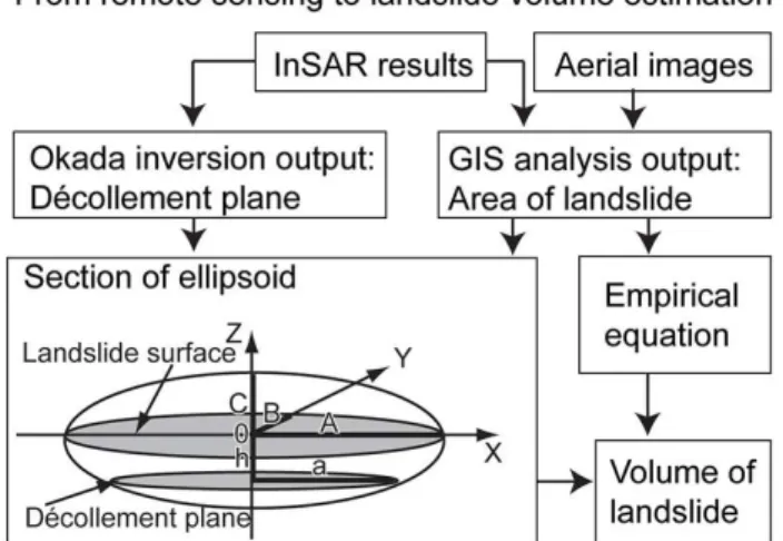
Fig. 3.A flow chart showing data and steps taken to estimate the landslide volume and a sketch of the geometric figure that we used for the volume calculation. “A” is the major axis of an ellipsoid in theX direction, “B” is the major axis of an ellipsoid in theY direction and “C” is the major axis of an ellipsoid in theZdirection. his the distance between the plane of the landslide surface and the sliding plane.ais the major axis in theXdirection of the sliding plane. The volume is calculated for the area enclosed between the plane of the landslide surface and the sliding plane.
tools. The area and perimeter of the landslide boundary were further analysed in ArcMap.
Photography taken by a geotagging camera allowed an even closer view of the selected structures and their com-parison to InSAR data.
A larger view was possible due to Landsat imagery. After importing these image data to ArcGIS, we were able to visu-alise the growing extent of the mining activity and its effect on the displacement field.
3.4 Modelling
The sliding planes of a landslide play an important role in the activity of the landslide (Petley et al., 2002; Petley et al., 2005). Knowledge of the location, shape and the size of the sliding plane allows estimation of the landslide volume. To investigate the geometry of the sliding plane of the observed displacement, we applied inverse modelling techniques. Dis-placement maps produced from the InSAR data were used as input data. We followed previous kinematic landslide studies (Fruneau et al., 1996; Martel, 2004) where models were used to describe landslide processes. These elastic models con-sider a flat earth and a linear elastic rheology. In our model, the main rupture plane of the landslide was simulated by a planar dislocation plane (Okada, 1985). We herein consid-ered this dislocation plane as a first-order approximation, be-cause the model is simplified in a geometric and a physi-cal sense. Geometriphysi-cally, the models are simplified as they rely on the half space assumption and the rectangular dislo-cation plane, with an upper edge being parallel to the
sur-face. Physically, the models are unrealistic as they rely on a linear elastic rheology and a dislocation along a plane. The dislocation plane we used has 8 unknowns: length, width, depth, two-dimensional position, dip and strike angles, and dip-slip dislocation components. We used the genetic algo-rithm to search the model and optimise the free parameters (Shirzaei and Walter, 2009), choosing a wide range of pos-sible solutions for the model parameters as a starting point. The genetic algorithm defines a cost function and initialises the genetic algorithm’s parameters.
We used this type of model because large landslides have structures similar to tectonic faults (Fleming and Johnson, 1989). Structures found inside a landslide (Fleming and Johnson, 1989) also motivated consideration of dislocation planes in translational landslide rupture models (Fruneau et al., 1996; Muller and Martel, 2000). We follow these previ-ous works by assuming that our observed displacement fields from InSAR may be simulated by planar dislocations within an isotropic elastic half-space. All InSAR deformation mea-surements were inverted to test the stability of the décolle-ment plane. Only model parameters that emerged when the genetic algorithm had stabilised, which means that the pa-rameters had not changed for several iterations, were consid-ered.
3.5 Estimation of landslide volume
A common way to calculate the rotational landslide volume is to assume that the soil mass has the shape of an ellipsoid (Cruden and Varnes, 1996; Marchesini et al., 2008). We ex-pand on this concept by considering a more complex and re-alistic landslide geometry: one containing both rotational and translational components. A translational component is con-sidered by an ellipsoid segment constrained by two parallel planes (Fig. 3). The lower plane is the décollement as in-verted from our InSAR data, and the upper plane reflects the surface expression of the landslide (Fig. 3). There are two semi-major axes, AandB. Consider the ellipsoid segment with décollement planez=h, wherehis the depth of slid-ing plane. This plane is parallel to the surface plane (XY ) located at depthh. The third vertical semi-major axisC can be calculated as follows:
a=A×
q
1−(h/C)2, (1)
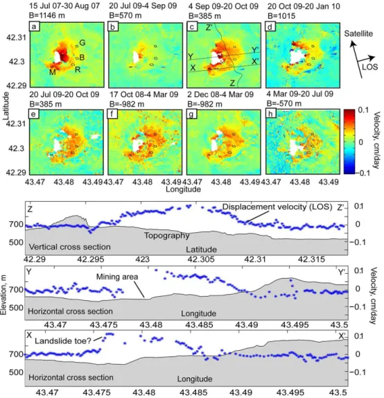
Fig. 4.Velocity (cm day−1) in the line-of-sight (LOS) direction from InSAR data. Given above each image are the two acquisition dates and
the spatial baselines (B). Interferograms that are temporally or spatially decorrelated are not shown. Black lines show the profiles on plot(c),
for which the topography and displacement velocities are shown below (Z-Z′, Y-Y′, X-X′). Polygons are marked with the letters “G”, “B”,
“R” and “M” (panela) and present areas where average velocities were calculated for Fig. 9.
V =
h Z
0
π×A×B×
1−z
2
C2
dz=π×A× (2)
B×
h− h
3
3×C2
.
An alternative way to evaluate the volume of a transla-tional or rotatransla-tional landslide is based on the landslide erosion rate (Hovius et al., 1997; Malamud et al., 2004; Larsen et al., 2010), where the predicted volumeV of a landslide of area Scan be approximated by the following empirical relation:
V =0.05×S1.3. (3)
The parameter 0.05 was determined empirically for soil landslides (Larsen et al., 2010). An exponent in the range
of 1.1–1.3 characterises a soil landslide (Edilashvili et al., 1974), similar to our case in Georgia.
The flow chart (Fig. 3) shows the steps that allow evaluat-ing landslide volumes usevaluat-ing the above-described methods.
4 Results
4.1 InSAR deformation field
Figure 4 shows the unwrapped and geocoded versions of the InSAR data set. The warm colours (positive values) indicate motion towards the satellite, while cold colours (negative val-ues) indicate motion away from the satellite (Fig. 4).
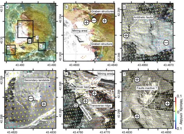
Fig. 5. (a)Aerial photography covered by a displacement map derived from InSAR.(b–f)details of the black boxes in(a), allowing a
comparison between the displacement map and the morphology. Red pixels show movement towards the satellite. See text for discussion.
hence approximately 2 km long (north–south) and 0.6 km wide (east–west). A similar pattern emerges from all interfer-ograms, which confirms the displacement occurrence. How-ever, the amplitude of the displacement varies, occasionally even if the same duration is bracketed by the data (Fig. 4a– c). This observation complicates the study because the land-slide process is found to be highly non-linear. The displace-ment velocity sharply increases in the interferogram from 4 September 2009 to 20 October 2009 and extends to almost the entire kidney-shaped landslide surface. The maximum difference between interferograms from 4 September 2009 to 20 October 2009 and 20 July 2009–4 September 2009 reaches 5 cm. We will provide more information about the possible reasons for different amplitudes in the discussion section.
Three profiles taken from one of the InSAR images (Fig. 4, profiles Z-Z′, Y-Y′, X-X′) clearly indicate that
no displacement was observed outside the landslide. The bulk of the landslide moves at similar rates, except that sharp gradients can be observed in the toe region. The gaps (Fig. 4, profiles Y-Y′) indicate areas of mining activity,
where no data are presented due to mining activity, steep topography or erosion.
4.2 Comparison of InSAR to optical images
The surface of the landslide is hummocky and fissured. We found several local protrusions and depressions on the land-slide body, which were also clear from the profile (Fig. 4, profiles Z-Z′, Y-Y′, X-X′). Figure 4c presents locations of
profiles (Fig. 4, profiles Z-Z′, Y-Y′, X-X′).
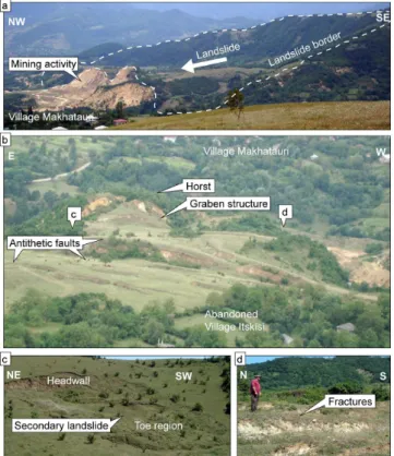
Fig. 6.View of the landslide from the northeast(a)and from the
back of the landslide, east–west(b). There are slopes cut by
min-ing activity in image(a). The white arrow shows the direction of landslide movement. The view of the landslide from the back(b)
shows landslide activity structures that are present in the aerial pho-tograph correlated with the InSAR signal in Fig. 5.(c)and(d)show
secondary landslides and fractures, respectively. Their positions are shown in image(b).
ridges, possibly associated with the landslide toe. Figure 5f presents an area where fault structures were observed in the field. However, the InSAR result does not show a signifi-cant displacement gradient, possibly indicating that the faults had not been active during the InSAR survey. The interfero-grams suggest that these and some of the fault areas are stable (Fig. 5a and f). It is likely that these landslide structures have either very low or no activity, or that any activity is masked by the high density of vegetation. These landslide structures are shown in both Fig. 5 and the survey photographs (Fig. 6). Because the InSAR data were available only in ascending orbits, a reconstruction of the absolute horizontal and ver-tical components of the displacement was not possible. We assume, however, that most of the motion is westward be-cause the morphology displays a slope orientation to the west (Fig. 6a). At localised regions, significant ground movement is detected at sites with slopes facing east, thus in the oppo-site direction. The observation that the movement is affecting both westward- and eastward-facing slopes may lead us to speculate that the type of movement is relatively deep seated and involves both synthetic and antithetic faults (Fig. 6b) to
Fig. 7.Simplified structural map of the Itskisi landslide. Contour
lines are based on SRTM DEM and have 30-metre intervals. The features mapped are presented in the legend. The possible body of the landslide is within the red line(a). The red dashed line shows
the landslide boundary detected from the morphology.(b)is a
de-tail of the black box in(a). Aerial photograph shows the fissured,
hilly surface of the landslide(c). Structures are well aligned with
the orientation of the Okada plane, as obtained from modelling of the landslide process (Fig. 8, Table 1, strike parameters).
form horst and graben structures. In other words, local mor-phologic features (Fig. 6c and d) and slopes have only minor influence on the moving mass, which is controlled instead by the large-scale topography and a deep-seated décollement.
Due to the slow rate of the landslide, the surface activ-ity of the sliding area is not clear in optical Landsat satellite imagery (Fig. 2). Investigation of high-resolution aerial pho-tographs, however, reveals further structural features such as folds, steps, lineaments, faults, outcrop sites and ponds (Fig. 7). We used these structural features to identify the type and complexity of movement for this landslide area.
Table 1.Output parameters from inversion model for different interferograms (Fig. 8a–c).
Case Temporal Length, Width, Depth, Dip Strike Dip-slip
baselines, days km km km m
a 46 1.45 0.8 0.19 −9◦ −36 −0.134
b 46 1.3 0.6 0.12 −8.2◦ −40 −0.17
c 92 1.37 0.67 0.14 −7.4◦ −39 −0.12
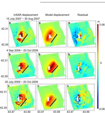
Fig. 8.Observed quantities (left), modelled quantities (middle) and
the residual (right). The mining activity was not accounted for in the modelling. The parameters of the model are given in Table 1.
trees or their remnants inside the ponds, which supports the idea that the ponds have appeared recently.
We identified visible scarps for this region from the aerial photograph and field observations (Fig. 7). The major areas of debris are on the eastern slope of the landslide. Over the course of our field season, the debris flow tracks, debris fan deposits and scars evolved. Newly formed cracks hidden by vegetation were found during field surveying.
The area affected by landslide processes was calculated in GIS using a polygon created based on InSAR, aerial pho-tography and field observations (Fig. 7). We found that the area of the kidney-shaped landslide identified by its mor-phology is approximately 2.9 km2, the perimeter of total area affected by the landslide is approximately 7.48 km, and the area having a displacement signal from InSAR is approxi-mately 0.9 km2.
4.3 Modelling results
We inverted the three best interferograms with temporal baselines of 46 or 92 days. Figure 8 shows the observed
displacements from InSAR data, model simulations of the same geometry and residuals that show the difference be-tween those two displacement fields. In all these data sets, the optimum décollement plane is sub-horizontal and dips slightly to the northwest. The residuals are generally less than 5 cm, which means that the signal was simulated very well and the residuals approach the noise level. The highest resid-ual is in the deposition zone of the landslide. Table 1 shows the output parameters for the model initiated with different values of input parameters. We detected a slight variation in the location and geometry of the sliding plane. For example, the dip ranges between−7◦ and−9◦ westward, the strike ranges between 35◦and 40◦northeast–southwest, the dip slip
ranges between−12 and−0.17 m to the northwest and the depth ranges from 120 to 190 m below the surface. As these inversions provide an indirect view on the décollement plane, we can now elaborate on the landslide volume.
4.4 Landslide volume
Using the ellipsoid segment concept, we calculated the ge-ometrically predicted volume based on the surface affected and the location of the décollement plane. We present dis-placement on the surface as an ellipse with semi-major axes A and B, which have values of 1 and 0.3 km, respectively (Fig. 3). The axisAis found from modelling as the length parameter (average 0.65 km) andhis the modelled depth of the detachment plane (average 0.12 km). Based on these pa-rameters and using Eq. (2), we estimated the volume of the Itskisi landslide to be 0.09 km3. We did not include dip in our volume estimation because the slope of the target area is approximately 10◦, which is similar to the dip angle of the
décollement as obtained from inverse modelling.
5 Discussion
In this work, only a limited satellite radar data set was avail-able. In Georgia this may result from a combination of po-litical sensitivities, lack of previous scientific interest, and acquisition conflicts with other study areas.
The remaining data, however, allowed us to obtain new insights into a specific landslide case in Georgia. Eight reli-able interferograms spanning over 3 years were produced to map the extent and amount of movement on the ground. Out of these, three interferograms have a noise level that makes them difficult to interprete, whereby up to 50 % of the ex-pected signal is attributed to noise. The remaining five inter-ferograms, however, were of a high and consistent quality.
In this work we speculate about the relationship between landslide acceleration and extrinsic processes. We note that although an earthquake occurred during the observation pe-riod, at a time coinciding with the largest landslide displace-ments in the InSAR data set, additional and complementary data at the landslide site would be needed to make a stronger case for a direct relationship between these events. As long as in-site observations are not made of the Itskisi landslide or similar landslides, a clear understanding of external triggers remains elusive. The same limitation also concerns rainfall data. No accurate weather data was available to us, which is why we herein used weather models instead of in-site rain gauge observation.
The relationship of a landslide area to anthropogenic ac-tivities, here meaning mining is a critical issue. Because the Itskisi landslide has destroyed the Itskisi village and is threat-ening others, liability issues restrict a great deal of scientific communication between ourselves and mine operators. In ad-dition, our own survey showed that not only one mining com-pany but at least 17 are involved in extracting sands from the landslide toe region, which makes a control on extraction rates and volume even more difficult. Here we relied more on satellite imagery (Landsat), which clearly show the vast spread of the area of effected by mining.
We use both InSAR and optical data for the detection and kinematic analysis of a landslide in Georgia. The landslide is 0.9 km2in area, subject to a motion of up to 6 cm within 46 days and affects a populated region and a major mining site. Although we use radar data from a single direction (as-cending satellite pass) only, the combination of InSAR dis-placement maps, aerial photography analysis and modelling provides information about the landslide dynamics. One of the important problems that may be encountered in the pro-cessing of radar images is the loss of coherence due to spatial or temporal factors. For this reason, we excluded some inter-ferograms from our analysis and modelling. In the following section, we discuss the effects of extrinsic processes, such as those related to rainfall, earthquake and mining activity, on landslide dynamics.
5.1 Impacts
The landslide may affect surrounding infrastructure, popula-tion and river flow. Landslide can dam river (Fig. 7), which may induce major hydrological hazards such as floods or the loss of drinking water resources. Landslide also affects ero-sion and can cause short-term losses of topsoil and vegeta-tion. Landslide damming has both short- and long-term ef-fects (Schuster and Highland, 2003). The Itskisi landslide di-rectly affected four villages: Itskisi, Makhatauri, Savane and Irtavaza (Fig. 10). The village of Itskisi was located directly on the landslide and moved downslope. Houses there were damaged, and most of the population left the village. The villages Savane and Makhatauri are separated by a river at the foot of landslide. In the scenario of landslide occurrence, the landslide may block a river and reach the village Savane, which is approximately 300 m away from the landslide area. The village Itavaza is located on the opposite slope of the landslide.
Understanding this type of landslide is therefore particu-larly important because eyewitnesses have reported increase in landslide hazards and risk over the past few decades.
5.2 Factors triggering landslides
A displacement signal is detected in each interferogram shown in Figure 4 and is particularly strong in interferograms with short temporal baselines. Because variation in the dis-placement rates affects only the kidney-shaped landslide area and not the stable surroundings, we conjecture that this vari-ation is not an artefact. The normalised velocity value sug-gests highly variable slip rates. The changes in the velocity may be due to variations in groundwater, which are a func-tion of rainfall intensity or seasonal water variafunc-tions such as snowmelt.
We select the average velocity at four different places on the landslide (Fig. 4a–h) to investigate the relationship be-tween changes in velocity and precipitation. We compare these velocities to average monthly precipitation data (Fig. 9 black curve), which are based on the atmospheric general circulation model ECHAM5 (http://www.mpimet.mpg.de). The spatial resolution is roughly equivalent to 2.8 degrees in both directions, latitude and longitude (Roeckner et al., 2003). The period from June 2007 to January 2010 has a maximum precipitation value of 150 mm. The interfero-grams from 17 October 2008 to 4 March 2009, 2 Decem-ber 2008 to 4 March 2009 and 20 OctoDecem-ber 2009 to 20 Jan-uary 2010 (Fig. 4) cover periods with monthly precipitation below 150 mm, while all other interferograms cover intervals with monthly precipitation less than 100 mm. The velocity in the interferogram from 2 December 2008 to 4 March 2009 is slightly higher (0.01 cm day−1) than in the interferogram
Fig. 9.Distribution of precipitation (black curve, left scale) based on ECHAM5. The coloured lines (green, blue, red) and bar graphs (magenta) show velocities (right scale) within the area identified by letters “R”, “G”, “B”, “M” in Fig. 4a.
average precipitation (Fig. 9). These interferograms cover the time from 20 July 2009 to 20 October 2009 and 15 July 2007 to 30 August 2007. Thus, the apparent acceleration of the landslide in September–October 2009 cannot be explained by rainfall.
Inspection of the global earthquake catalogue (CMT) shows that a magnitude Mw=6.0 earthquake on 7 Septem-ber 2009 occurred at 10 km depth and a distance of only ap-proximately 30 km from the landslide. On 18 July 2007, an-other earthquake occurred, this one with magnitude Ml=3.8 at 15 km depth (http://seismo.iliauni.edu.ge/) at a distance of 12 km. The observed increase of the displacement rates at these times suggests that these earthquakes may have had a triggering influence. Such a triggering influence is in agree-ment with work by Jibson et al. (1994), where numerous landslides were triggered following an earthquake at a dis-tance of approximately 30 km.
These discussions are relevant given the ongoing mining activity during the period of this study. There is 68.07 Ha of mining area covered by 17 mining companies (source: www.gwp.org, licenses issued for the use of mineral re-sources in Georgia), as shown in Fig. 2 (bright areas). These images do not allow clear analysis of the landslide, but they do show the development of mining activity (Fig. 2, bright areas). Quartz sand extraction began in 1968 and accelerated greatly in 2007, reaching rates that continue today. This may explain why the points closest to the active mines show the highest velocities in 2007 (Fig. 9, margin line, year 2007).
We conclude that the landslide may have been triggered by rainfall, earthquakes and the man-made removal of the toe. Unfortunately, due to the lack of good topographic data, ground data and field information at that time, no clear rela-tion between the earthquakes and the triggering of the land-slide movements could be found.
Fig. 10. (a)Three-dimensional GIS visualisation showing
InSAR-measured displacements in cm (4 April 2009–20 October 2009) on a digital elevation surface (ASTER, resolution 30 m) combined with an aerial photograph. The area is 3.5 km east–west by 4.8 km north– south in size. The colour scale bar indicates displacement. Four vil-lages were affected by the landslide.(b)The profile along the region of interest runs west–east along theX−X′transect shown in(a).
The colour scale for the profile points is the same as for the 3-D vi-sualisation above. The vectors are directed to the line-of-sight. The length of the vector indicates the magnitude of the displacement, which was artificially increased by a factor of 100 for better visi-bility. The slip plane for the Itskisi landslide is estimated based on results from remote sensing, field observations and modelling. Our model favours the landslide to be complex, with both a translational part (Okada model) and rotational elements (dashed red curves).
5.3 Conceptual model
Our structural mapping and analysis of InSAR data suggest that several smaller sliding blocks combine to form the larger landslide complex. We applied a model to study the internal geometry of the landslide.
the Slumgullion landslide in Colorado (Gomberg and Bodin, 1995). In our model, we had to ignore parameters that may play important roles in the development of the landslide pro-cess. We did not consider possible material heterogeneity, nor did we take into account topography or the distributions of possible driving forces and gravitation. Our model also does not show the evolution of a landslide and secondary slides and has difficulty predicting the true shape of the slid-ing plane. However, in the first approximation, the model selects the potential sliding plane most susceptible to fail-ure from an infinite number of potential surfaces. In addi-tion, translational slides can be connected to upslope and downslope rotational slides (Fig. 10). The lengths of the dis-placement vectors remain the same at certain areas (Fig. 10, profile), and the distribution of the displacement vectors is a function of the slip-surface sliding plane (Casson et al., 2005). The equal displacement vectors in the centre zone of the landslide indicate a uniform translational landslide there (Casson et al., 2005). However, the lengths of the displace-ment vectors increase from east to west, which implies the presence of rotational landslide elements in the upper zone (Fig. 10, profile).
The complete picture of the landslide therefore consists of a planar (translational) fault at depth that curved toward the toe and headwall to form a combined rotational-translational landslide body. Secondary landslides developed and mi-grated, piggybacking on each other. Antithetic faults and horst and graben structures developed. The grabens formed ponds and destroyed the Itskisi village, whereas the horst structures are currently exploited by mining activity. A lo-cal girdle of subsidence surrounding the mine highlights the effects of the loss of toe support. Landslides may be triggered by mining intensification (as in 2007) or earthquakes (as in 2009). A direct link to rainfall was not found, though we note that the rainfall database was poor.
Previous studies show the efficiency of combining differ-ent remote sensing images for monitoring and characteris-ing landslide processes (Strozzi et al., 2005; Casson et al., 2005). Using both radar and optical satellite images allows us to trace the behaviour of landslides in space and time and to evaluate an area affected by possible landslides. A concep-tual model was developed based on observational data from remote sensing (Casson et al., 2005). The aim of the concep-tual model is the evaluation of the volume of possible land-slides for the hazard mass movement.
6 Conclusions and perspective
Landslides in the area of the Caucasus Mountains are not well monitored due to the high costs and difficult logistics of doing so. As we demonstrate, the combination of InSAR data, aerial photography analysis, Landsat imagery and other information allows us to identify and monitor a landslide in the centre part of Georgia. The displacement rate of the
land-slide is from 10 cm year−1to 30 cm year−1, covering an area
of approximately 0.9 km2. Our data suggest that the landslide movement is not stable, occasionally displaying a significant acceleration. These episodes of high landslide mobility may be associated with potential external triggering mechanisms, such as rainfall, man-made activity or a tectonic earthquake. We characterise the landslide movement and determine displacement velocities within the landslide body. By com-bining this work with modelling, we are able to more pre-cisely explore the dimensions and detachment plane geome-try and further illuminate potential hazards and environmen-tal interactions. The maximum depth of the landslide detach-ment plane ranges from 0.12 to 0.19 km.
Field observations show good correlation of surface frac-tures and the displacements obtained from InSAR data (Figs. 5 and 6). We identify a number of factors that may trigger landslides. Mining caused a loss of mass in the toe. The intensification of mining exploration locally increased the landslide velocity. In addition, the most dramatic veloc-ity increase was found in association with a Mw=6.0 earth-quake located 30 km from the landslide.
This landslide poses threats to human lives and structures that support transportation and natural resource management in four villages. The landslide or its part may be activated given the proximity (∼30 km) of a possible focus of a strong earthquake (Keefer 1994; Wasowski, 2002).
This finding has important implications for hazard assess-ment because the location and type of landslides in Georgia apparently vary in time. The mining industry, which provides and improves infrastructure and prosperity in the region, also may contribute to triggering landslides.
Over the past 30 years, the use of remote sensing tech-niques in the geosciences has increased dramatically. The number of satellites with various temporal and spatial reso-lutions, bands and broad coverage has also increased. In this regard, there is greater opportunity to explore an event with various data sets. The probability of data being available for unexpected geological disasters is also higher. This remote sensing development plays a major role for creating a data archive for Georgia, where high hazards exist but only small numbers of observational tools are used.
The results of this study demonstrate that complex remote sensing techniques have the potential to become good tools for early warning of landslide disasters. Satellite data al-low monitoring landslides in space and time. The displace-ment distribution obtained from InSAR data can be used in a model to characterise the geometry and spatial evolution of the landslide slip surface. Its temporal evolution can also be investigated with remote sensing data.
on landsliding may even augment more risk as unloading in the toe region continues. Moreover, as the landslide is hence further developing, also interacting processes, such as earth-quake or rainfall triggering may alter with time. Therefore, close observation and further work with a more regular data acquisition are needed, allowing detection of displacement rate changes at higher detail. Also, monitoring of mining tivity may also help to clarify the impact that man-made ac-tions have on natural hazards. In this view, the Itskisi land-slide may provide an excellent laboratory, where such inter-acting and cascading processes might be well studied.
Acknowledgements. The authors would like to thank the DAAD
(German Academic Exchange Service) for financially supporting the PhD research of Elena Nikolaeva, the Institute of Earth Sciences at Ilia State University in Tbilisi (Georgia) for organi-sation of fieldwork and providing aerial photographs, Henriette Sudhaus and Hannes Bathke for their valuable advice during the processing of radar data and Michele Pantaleo for geology dis-cussions. Financial support also came from the HGF Alliance EDA.
The service charges for this open access publication have been covered by a Research Centre of the Helmholtz Association.
Edited by: P. Tarolli
Reviewed by: two anonymous referees
References
Canuti, P., Casagli, N., Catani, F., Falorni, G., and Farina, P.: In-tegration of Remote Sensing Techniques in Different Stages of Landslide Response, Prog. Landslide Sci., 251–260, 2007. Cardenal, J., Mata, E., Delgado, J., Hernandez, M. A., and
Gonza-lez, A.: Close range digital photogrammetry techniques applied to landslides monitoring, Int. Arch. Photogramm. Remote Sens. Spat. Inf. Sci., XXXVII, 235–240, 2001.
Casson, B., Delacourt, C., and Allemand, P.: Contribution of multi-temporal remote sensing images to characterize landslide slip surface? Application to the La Clapière landslide (France), Nat. Hazards. Earth Syst. Sci., 5, 425–437, doi:10.5194/nhess-5-425-2005, 2005.
Chen, C., Zhang, J., and Lu, L.: Identification of Layover and Shadow Regions in InSAR Image, 2011 Int. Symp. Image Data Fusion, IEEE, 1–4, 2011.
Chen, C. W. and Zebker, H. A.: Phase unwrapping for large SAR in-terferograms: Statistical segmentation and generalized network models, IEEE Trans. Geosci. Remote Sens., 40, 1709–1719, 2002.
Chudnovsky, A. and Ben-Dor, E.: Application of visible, near-infrared, and short-wave infrared (400–2500 nm) reflectance spectroscopy in quantitatively assessing settled dust in the indoor environment. Case study in dwellings and office environments, Sci. Total Environ., 393, 198–213, 2008.
Colesanti, C., Ferretti, A., Novali, F., Prati, C., and Rocca, F.: SAR monitoring of progressive and seasonal ground deformation
us-ing the permanent scatterers technique, IEEE Trans Geosci. Re-mote Sens., 41, 1685–1701, 2003a.
Colesanti, C., Ferretti, A., Prati, C., and Rocca, F.: Monitoring land-slides and tectonic motions with the Permanent Scatterers Tech-nique, Eng. Geol., 68, 3–14, 2003b.
Colesanti, C. and Wasowski, J.: Investigating landslides with space-borne Synthetic Aperture Radar (SAR) interferometry, Eng. Geol., 88, 173–199, doi:10.1016/j.enggeo.2006.09.013, 2006. Cruden, D. M.: The geometry of slip surfaces beneath
land-slides: predictions from surface measurements: Discussion. Can. Geotech. J., 23, p. 94, doi:10.1139/t86-012, 1986.
Cruden, D. M. and Varnes, D. J.: Landslide types and processes, in: Landslides – Investigation and Mitigation, edited by: Turner, A. T., Schuster, R. L., Transp. Res. Board, Spec. Rep., 247, 36–75, doi:10.1007/BF02590167, 1996.
Delacourt, C., Allemand, P., Berthier, E., Raucoules, D., Casson, B., Grandjean, P., Pambrun, C., and Varel, E.: Remote-sensing tech-niques for analysing landslide kinematics: a review, Bull. Soc. Geol. Fr., 178, 89–100, doi:10.2113/gssgfbull.178.2.89, 2007. Edilashvili, V. Y. Y., Lekvinadze, R. D., and Gogiberidze, V. V.:
Effect of tectonics on manganese accumulation in Georgia, Int. Geol. Rev., 16, 37–41, doi:10.1080/00206817409471856, 1974. Fleming, R. W. and Johnson, A. M.: Structures associated with strike-slip faults that boundlandslide elements, Eng. Geol., 27, 39–114, doi:10.1016/0013-7952(89)90031-8, 1989.
Fruneau, B., Achache, J., and Delacourt, C.: Observation and mod-elling of the Saint-Étienne-de-Tinée landslide using SAR inter-ferometry, Tectonophysics, 265, 181–190, doi:10.1016/S0040-1951(96)00047-9, 1996.
Gamkrelidze, I. and Shengelia, D.: Pre-Alpine Geodynamics of the caucasus, Suprasubduction Regional Metamorphism and Gran-itoid Magmatism, Bull. Georg. Natl. Acad. Sci., 175, 57–65, 2007.
García-Davalillo, J. C., Herrera, G., Notti, D., Strozzi, T., and Álvarez-Fernández, I.: DInSAR analysis of ALOS PALSAR im-ages for the assessment of very slow landslides: the Tena Valley case study, Landslides, doi:10.1007/s10346-012-0379-8, 2013. Goldstein, R. M. M. and Werner, C. L. L.: Radar interferogram
filtering for geophysical applications, Geophys. Res. Lett., 25, 4035–4038, 1998.
Gomberg, J. and Bodin, P.: Landslide faults and tec-tonic faults, analogs?: The Slumgullion earthflow, Colorado. Geology, 23, 41–44, doi:10.1130/0091-7613(1995)023<0041:LFATFA>2.3.CO;2, 1995.
Gracheva, R. and Golyeva, A.: Landslides in mountain regions: hazards, resources and information, in: Geophys. Hazards, Int. Year Planet Earth, edited by: Beer, T., Springer Netherlands, Dor-drecht, 249–260, 2010.
Guzzetti, F., Manunta, M., Ardizzone, F., Pepe, A., Cardinali, M., Zeni, G., Reichenbach, P., and Lanari, R.: Analysis of Ground Deformation Detected Using the SBAS-DInSAR Technique in Umbria, Central Italy, Pure Appl. Geophys., 166, 1425–1459, 2009.
Guzzetti, F., Mondini, A. C., Cardinali, M., Pepe, A., Cardinali, M., Zeni, G., Reichenbach, P., and Lanari, R.: Landslide inventory maps: New tools for an old problem, Earth-Science Rev., 112, 42–66, 2012.
Highland, L. M. and Bobrowsky, P.: The Landslide Handbook – A Guide to Understanding Landslides, Landslides, 129 pp., 2008. Hilley, G. E., Bürgmann, R., Ferretti, A., Novali, F., and Rocca, F.:
Dynamics of slow-moving landslides from permanent scatterer analysis, Science, 304, 1952–5, 2004.
Hovius, N., Stark, C. P., and Allen, P. A.: Sediment flux from a mountain belt derived by landslide mapping, Geology, 25, 231– 234, 1997.
Jaboyedoff, M., Oppikofer. T., Abellán, A., Derron, M.-H., Loye, A., Metzger, R., and Pedrazzini, A.: Use of LIDAR in landslide investigations: a review, Nat. Hazards., 61, 5–28, 2010. Jibson, R. W., Randall, W., and Prentice, C. S.: Ground Failure
Pro-duced by the 29 April 1991 Racha Earthquake in Soviet Georgia, US Geol. Surv., 10, Open-File Report 91-392, ii, 5 leaves, 1991. Jibson, R. W., Prentice, C. S., Borissoff, B. A., Rogozhin, E. A., and Langer, C. J.: Some observations of landslides triggered by the 29 April 1991 Racha earthquake, Republic of Georgia, Bull. Seismol. Soc. Am., 84, 963–973, 1994.
Kampes, B. and Usai, S.: Doris: The Delft object-oriented radar interferometric software, 2nd Int Symp Oper Remote Sens En-schede Netherlands, 1–4, doi:10.1.1.46.1689, 1999.
Keefer, D. K.: The importance of earthquake-induced landslides to long-term slope erosion and slope-failure hazards in seismically active regions, Geomorphology, 10, 265–284, 1994.
Larsen, I. J., Montgomery, D. R., and Korup, O.: Landslide erosion controlled by hillslope material, Nat. Geosci., 3, 247–251, 2010. Leonov, M. G.: Fractures in the Dzirula massif (Georgia), Int. Geol.
Rev., 18, 1019–1024, 1976.
Malamud, B. D., Turcotte, D. L., Guzzetti, F., and Reichenbach, P.: Landslide inventories and their statistical properties, Earth Surf Proc. Landforms, 29, 687–711, 2004.
Martel, S.: Mechanics of landslide initiation as a shear fracture phe-nomenon, Mar. Geol., 203, 319–339, 2004.
Martha, T. R., Kerle, N., Jetten, V., van Westen, C. J., and Kumar, K. V.: Characterising spectral, spatial and morphometric properties of landslides for semi-automatic detection using object-oriented methods, Geomorphology, 116, 24–36, 2010.
Muller, J. R. and Martel, S. J.: Numerical Models of Translational Landslide Rupture Surface Growth, Pure Appl. Geophys., 157, 1009–1038, 2000.
Nadim, F., Kjekstad, O., Peduzzi, P., Herold, C., and Jaedicke, C.: Global landslide and avalanche hotspots, Landslides, 3, 159–173, 2006.
Nichol, J. and Wong, M. S.: Satellite remote sensing for detailed landslide inventories using change detection and image fusion, Int. J. Remote Sens., 26, 1913–1926, 2005.
Okada, Y.: Surface deformation due to shear and tensile faults in a half-space, Int. J. Rock Mech. Min. Sci. Geomech. Abstr., 75, 1135–1154, 1985.
Ouimet, W. B.: Landslides associated with the May 12, 2008 Wenchuan earthquake: Implications for the erosion and tectonic evolution of the Longmen Shan, Tectonophysics, 491, 244–252, 2010.
Perski, Z., Hanssen, R., Wojcik, A., and Wojciechowski, T.: InSAR analyses of terrain deformation near the Wieliczka Salt Mine, Poland, Eng. Geol., 106, 58–67, 2009.
Petley, D. N., Bulmer, M. H., and Murphy, W.: Patterns of move-ment in rotational and translational landslides, Geology, 30, 719– 722, 2002.
Petley, D. N., Mantovani, F., Bulmer, M. H., and Zannoni, A.: The use of surface monitoring data for the interpretation of landslide movement patterns, Geomorphology, 66, 133–147, 2005. Principe, J. C., De Vries, B., De Oliveira, P. G., De Vries, B., and
De Oliveira, P. G.: The gamma-filter-a new class of adaptive IIR filters with restricted feedback, IEEE Trans Sig. Proc., 41, 3378– 3393, 2004.
Qi, S., Xu, Q., Lan, H., De Vries, B., and De Oliveira, P. G.: Spa-tial distribution analysis of landslides triggered by 2008.5.12 Wenchuan Earthquake, China. Eng. Geol., 116, 95–108, 2010. Riedel, B. and Walther, A.: InSAR processing for the recognition of
landslides, Adv. Geosci., 14, 189–194, 2008, http://www.adv-geosci.net/14/189/2008/.
Roeckner, E., Bäuml, G., Bonaventura, L., Brokopf, R., Kornblueh, M., Giorgetta, M., Hagemann, S., Kirchner, I., Tompkins, E., Manzini, A., Rhodin, U., Schlese, U., and Schulzweida, A.: The atmospheric general circulation model ECHAM5 – Part I: Model description, 349 pp., 2003.
Sandwell, D. T., Myer, D., Mellors, R., Shimada, M., Brooks, B., and Foster, J.: Accuracy and Resolution of ALOS Interferometry: Vector Deformation Maps of the Father’s Day Intrusion at Ki-lauea, IEEE Trans. Geosci. Remote Sens., 46, 3524–3534, 2008. Schulz, W. H.: Landslides mapped using LIDAR imagery, North, 4,
11 pp., 2004.
Schuster, R. L. and Highland, L. M.: Impact of landslides and inno-vative landslide-mitigation measures on the natural environment, Geol. Hazards Team, US Geol., 2003.
Shirzaei, M. and Walter, T. R.: Randomly iterated search and sta-tistical competency as powerful inversion tools for deformation source modeling: Application to volcano interferometric syn-thetic aperture radar data, J. Geophys. Res., 114, 1–16, 2009. Shirzaei, M. and Walter, T. R.: Estimating the Effect of Satellite
Orbital Error Using Wavelet-Based Robust Regression Applied to InSAR Deformation Data, IEEE Trans. Geosci. Remote Sens., 49, 4600–4605, 2011.
Strozzi, T., Farina, P., Corsini, A., Ambrosi, C., Thüring, M., Zil-ger, J., Wiesmann, A., Wegmüller, U., and Werner, C.: Survey and monitoring of landslide displacements by means of L-band satellite SAR interferometry, Landslides, 2, 193–201, 2005. Strozzi, T., Ambrosi, C., and Raetzo, H.: Interpretation of Aerial
Photographs and Satellite SAR Interferometry for the Inventory of Landslides, Remote Sens., 5, 2554–2570, 2013.
Tofani, V., Segoni, S., Agostini, A., Catani, F., and Casagli, N.: Technical Note: Use of remote sensing for landslide stud-ies in Europe, Nat. Hazards. Earth Syst. Sci., 13, 299–309, doi:10.5194/nhess-13-299-2013, 2013.
Van Westen, C. J., Straatsma, M. W., Turdukulov, U. D., Feringa, W. F., Sijmons, K., Bakhtadze, K., Janelidze, T., and Kheladze, N.: Atlas of Natural Hazards and Risk in Georgia, CENN Caucasus Environmental NGO Network, 2012.