Landslide dynamics and coupling revealed by L-band InSAR in central Georgia

(1)

NHESSD

1, 4925–4962, 2013

Landslide dynamics and coupling revealed by L-band

InSAR

E. Nikolaeva et. al

Title Page

Abstract Introduction

Conclusions References

Tables Figures

◭ ◮

Back Close

Full Screen / Esc

Printer-friendly Version Interactive Discussion

Discussion

P

a

per

|

D

iscussion

P

a

per

|

Discussion

P

a

per

|

Discuss

ion

P

a

per

|

Nat. Hazards Earth Syst. Sci. Discuss., 1, 4925–4962, 2013 www.nat-hazards-earth-syst-sci-discuss.net/1/4925/2013/ doi:10.5194/nhessd-1-4925-2013

Geoscientiic Geoscientiic

Natural Hazards and Earth System Sciences

Open Access

Discussions

This discussion paper is/has been under review for the journal Natural Hazards and Earth System Sciences (NHESS). Please refer to the corresponding final paper in NHESS if available.

Landslide dynamics and coupling

revealed by L-band InSAR in central

Georgia

E. Nikolaeva1, T. R. Walter1, M. Shirzaei1,*, and J. Zschau1 1

Department 2 – Physics of the Earth, Helmholtz Center Potsdam – GFZ German Research Center of Geosciences, Potsdam, Germany

*

now at: School of Earth and Space Exploration, Arizona State University, Tempe, AZ 85287-6004, USA

Received: 21 August 2013 – Accepted: 4 September 2013 – Published: 17 September 2013

Correspondence to: E. Nikolaeva ([email protected])

(2)

NHESSD

1, 4925–4962, 2013

InSAR

E. Nikolaeva et. al

Title Page

Tables Figures

◭ ◮

Back Close

Full Screen / Esc

Discussion

P

a

per

|

D

iscussion

P

a

per

|

Discussion

P

a

per

|

Discuss

ion

P

a

per

|

Abstract

The republic of Georgia is a mountainous and tectonically active area that is vulnerable to landslides. Because landslides are one of the most devastating natural hazards, their detection and monitoring is of great importance. In this study we report on a previously unknown landslide in central Georgia at the site of the village of Itskisi near

5

the town of Sachkhere. We used a set of ALOS PALSAR data to generate displacement maps using Interferometric Synthetic Aperture Radar (InSAR). We detected a sliding zone of dimensions 2 km north-south by 0.6 km east-west that threatens four villages. We estimated surface displacement of up to∼30 cm yr−1 over the sliding body in the

satellite line-of-sight (LOS) direction, with the greatest displacement occurring after a

10

local tectonic earthquake. We mapped the morphology of the landslide mass by aerial photography and field surveying. We found a complex set of interacting processes, including surface fracturing, shear and normal faults at both the headwall and the sides of the landslide, local landslide velocity changes, earthquake-induced velocity peaks, and loss in toe support due to mining activity. Important implications that are applicable

15

elsewhere can be drawn from this study of coupled processes.

We used inverse dislocation modelling to find a possible dislocation plane resembling the landslide basal decollement, and we used that plane to calculate the volume of the landslide. The results suggest a decollement at∼120 m depth dipping at ∼10◦

sub-parallel to the surface, which is indicative of a translational-type landslide.

20

1 Introduction

1.1 Landslides in Georgia

Landslides and related hazards are widespread in Georgia (Nadim et al., 2006; Gracheva and Golyeva, 2010) and cause substantial damage annually (Van Westen et al., 2012). The steep hill slopes, active geology and conditionally wet or even

(3)

NHESSD

1, 4925–4962, 2013

InSAR

E. Nikolaeva et. al

Title Page

Tables Figures

◭ ◮

Back Close

Full Screen / Esc

Discussion

P

a

per

|

D

iscussion

P

a

per

|

Discussion

P

a

per

|

Discuss

ion

P

a

per

|

tropical climatic conditions in Georgia (Van Westen et al., 2012) are important factors that contribute to the high landslide susceptibility there. Over 53 000 landslides have been identified, ranging from small-scale slumps to large-scale mass wasting of en-tire hillsides (Van Westen et al., 2012). Approximately 700 of those landslides have been identified through yearlong mapping and field work activities. A recent landslide

5

susceptibility analysis based on geology, slope classification and land cover mapping suggested that approximately 17 % of Georgia is located in high-hazard zones, and an-other 38 % is located in moderate-hazard zones (Van Westen et al., 2012). Landslide concentration is especially high and covers all scales in Adzharia, a region in south-western Georgia with a humid subtropical climate, with occurrence peaking in spring

10

and during summer storms (Gracheva and Golyeva, 2010).

Together with the steep topography and wet climate, tectonics can be a significant trigger of landslides. The Ms 7.0 earthquake on 29 April 1991, for instance, triggered numerous landslides and caused a loss of infrastructure and life (Jibson et al., 1994). Some of these landslides were known to be active already, but moving slowly. For

15

example, the slow-moving Chordi landslide accelerated and destroyed the village of Chordi shortly after the earthquake. This case highlights the importance of monitor-ing slow-movmonitor-ing landslides that may accelerate due to unpredictable external triggers. Slow-moving landslides in Georgia in particular can accelerate abruptly, especially if extrinsic factors act as triggers (Gracheva and Golyeva, 2010). However, the interplay

20

among various triggering factors has not been thoroughly investigated.

Although geologic mapping has been performed for some of these landslides, dy-namic and kinematic analyses of them have received little scientific attention. As will be shown in this work, space-based data allow analysis of displacement rates and the identification of possible detachment planes of a landslide, which, together with aerial

25

(4)

NHESSD

1, 4925–4962, 2013

InSAR

E. Nikolaeva et. al

Title Page

Tables Figures

◭ ◮

Back Close

Full Screen / Esc

Discussion

P

a

per

|

D

iscussion

P

a

per

|

Discussion

P

a

per

|

Discuss

ion

P

a

per

|

1.2 Landslide classification and hazards

Some 35 yr ago, landslides were first classified based on specific variables, such as the type of movement and type of material (Varnes, 1978).

The dynamics, i.e., the appearance and displacement pattern of a landslide, are pri-marily controlled by the geometry of the sliding planes (Cruden, 1986). These planes

5

are made up of a combination of basal decollements and laterally delimiting fractures. The decollement is usually not directly visible and is also difficult to infer from remote sensing techniques. Therefore, little is known about the geometric complexities and dynamics of active decollement planes. The laterally delimiting fractures, in turn, are visible at the surface and commonly include a headwall fault, which is the surface

ex-10

pression of the main detachment, en echelon sets of strike-slip and normal faults on either side with opposite senses and a compressional zone in the landslide toe that forms thrust and fold belts. The geometry of these sliding planes affects the different types of movement. Movement of a landslide can be translational, rotational, or com-plex (Cruden and Varnes, 1996). Rotational landslides move generally downward and

15

outward and are thought to be structurally confined by a curved basal detachment plane (Highland and Bobrowsky, 2008). Translational slides move hillslope-parallel and are structurally defined by a planar detachment slope-parallel plane (Highland and Bobrowsky, 2008). Most landslides likely involve a combination of rotational and trans-lational mechanisms. Because the network of these structures delimits the mass of a

20

landslide, structural characterisation of a landslide is important for assessing the land-slide volume. Landland-slide volume is the total the volume of displaced material in the depletion and accumulation zones.

The appearance of a landslide may depend on the type of material involved, such as the porosity contrast between soil and rock (Iverson et al., 2000). Some granular

mate-25

(5)

NHESSD

1, 4925–4962, 2013

InSAR

E. Nikolaeva et. al

Title Page

Tables Figures

◭ ◮

Back Close

Full Screen / Esc

Discussion

P

a

per

|

D

iscussion

P

a

per

|

Discussion

P

a

per

|

Discuss

ion

P

a

per

|

Landslides exhibit a wide range in velocity, from extremely slow (10−_{mm yr}−1_{) to}

extremely rapid landslides (10 m s−1_{) (Cruden and Varnes, 1996). This broad velocity}

range highlights a common problem in landslide monitoring: the ability to detect and explore several scales of displacement magnitude. This problem is described further in the following section.

5

1.3 Landslide detection and displacement monitoring

Most active landslides are studied using field-based morphological, structural and kine-matic analyses. Ground-based techniques are not appropriate for detecting a landslide in a broad area because of their time and financial costs. Non-intrusive remote sens-ing techniques have therefore become widely used for the detection and mappsens-ing of

10

the position, size and shape of landslides (Cardenal et al., 2001; Guzzetti et al., 2012) and potentially unstable slopes (Colesanti and Wasowski, 2006; Ouimet, 2010). Re-mote sensing techniques have specifically contributed to define states of activity, to monitor landslides, to improve hazard analysis and to allow implementation in early warning systems (Canuti et al., 2007). Remote sensing methods include aerial

pho-15

tographs, multispectral optical images (Qi et al., 2010), di_fferential Digital Elevation Models (DEMs) (Casson et al., 2005), interferometric analysis of radar images (Riedel and Walther, 2008) and LIDAR data (Schulz, 2004; Jaboyedoffet al., 2010) and others. The most commonly used method for landslide detection is the visual interpreta-tion of optical images (Tofani et al., 2013). Change detecinterpreta-tion techniques (Nichol and

20

Wong, 2005) and classification with semi-automated object-oriented methods (Martha et al., 2010) in optical imagery allow for landslide mapping. Together with detection, these methods allow monitoring and reconstruction of yearlong time series. For in-stance, rapid and large morphometric changes can be quantified using change detec-tion methods applied to high-resoludetec-tion optical data (Nichol and Wong, 2005). Airborne

25

(6)

NHESSD

1, 4925–4962, 2013

InSAR

E. Nikolaeva et. al

Title Page

Tables Figures

◭ ◮

Back Close

Full Screen / Esc

Discussion

P

a

per

|

D

iscussion

P

a

per

|

Discussion

P

a

per

|

Discuss

ion

P

a

per

|

2007). The combination of these methods is also used to improve landslide inventory maps (Guzzetti et al., 2012).

Interferometric Synthetic Aperture Radar (InSAR) techniques allow mapping of ground movement that occurs between two acquisition times (Hanssen, 2001). InSAR techniques are increasing in popularity for landslide applications (Colesanti and

Wa-5

sowski, 2006; Riedel and Walther, 2008; Tofani et al., 2013) as they are low-cost, al-most globally applicable, high-resolution and independent of day or night. The common InSAR method allows the detection and monitoring of slow (several cm per year) land-slides, following the classifications of Cruden and Varnes (1996). Persistent Scatterers SAR Interferometry (PS-InSAR) and Small Baseline Subset (SBAS) techniques allow

10

analysis of the temporal and spatial evolution of extremely slow landslides (several mm per year) (Colesanti et al., 2003; Hilley et al., 2004; Guzzetti et al., 2009). Combina-tions of different InSAR techniques are useful to detect and investigate different rates of landslides (Perski et al., 2009; García-Davalillo et al., 2013).

Each of these techniques has its advantages and disadvantages. Combining optical

15

and radar techniques creates good conditions for the study of landslides (Strozzi et al., 2013). In this work, we exploit aerial optical, satellite spectral and, foremost, InSAR data to analyse the dynamics and changes of a landslide.

2 Study area

We concentrate our study on a site located in the central western part of Georgia

20

(42.30◦_{N, 43.48}◦_{E) because of the known landslide potential, slope angle and field}

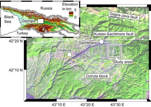
ac-cess there. We use a specific constellation to investigate the effect of extrinsic forcing (Fig. 1). Geologically, the region belongs to the Dzirula block, which is a topographic feature of the Chiatura formation (Gamkrelidze and Shengelia, 2007) (Fig. 1). The ge-ologic Chiatura formation was created by sedimentary deposition, with a sequence

25

(7)

NHESSD

1, 4925–4962, 2013

InSAR

E. Nikolaeva et. al

Title Page

Tables Figures

◭ ◮

Back Close

Full Screen / Esc

Discussion

P

a

per

|

D

iscussion

P

a

per

|

Discussion

P

a

per

|

Discuss

ion

P

a

per

|

siliceous sedimentary rocks to the west and shales and shaley sandstones to the east (Edilashvili et al., 1974; Leonov, 1976).

The relief profile of the study area shows a gently sloping morphology. The height varies only from 500 to 850 m; thus the slope is moderate, with slope angles less than 20◦_{. A significant part of the lower landslide flank is subject to mining activity (Fig. 2),} 5

where quartz sand is excavated. The nearby Kutaisi-Sachkhere thrust fault, located just

∼5 km to the north of the landslide area (Gamkrelidze and Shengelia, 2007), is thought

to be active (Seismic Catalogue of Georgia, http://seismo.ge) and thus has the potential to be an unpredictable landslide trigger (Fig. 1). Other faults at larger distances may also dynamically trigger the landslide.

10

3 Data and methods

3.1 Data

Data analysed comprise (a) satellite radar observations, (b) optical Landsat data and aerial photographs, (c) digital elevation data and (d) field inspection. The main focus of this work is on the satellite radar observations and interferometric processing.

15

To generate the InSAR maps, we considered 12 the Phased Array type L-band Synthetic Aperture Radar (PALSAR) acquisitions from the Advanced Land Observing Satellite (ALOS). In standard interferometry, the quality of the SAR signals degrades due to changes in the backscattering properties of the surfaces (e.g. vegetation), which is less critical in L-band sensors (Strozzi et al., 2005). The ALOS archives of our study

20

area contain only data acquired in ascending orbits, track 582 and frame 840, which means that the ground is observed by the satellite only from the west. The dataset spans the period from July 2007 through June 2010. Five images are high-resolution single-polarisation (Fine Mode Single (FMS) polarisation) mode and 7 images are high-resolution, dual-polarisation (Fine Beam Double (FBD) polarisation) mode. The range

25

(8)

reso-NHESSD

1, 4925–4962, 2013

InSAR

E. Nikolaeva et. al

Title Page

Tables Figures

◭ ◮

Back Close

Full Screen / Esc

Discussion

P

a

per

|

D

iscussion

P

a

per

|

Discussion

P

a

per

|

Discuss

ion

P

a

per

|

lution is 5 m for both modes. To avoid decorrelation associated with snow cover, we excluded scenes acquired in winter periods. The periods between master and slave images range from 46 to 138 days. The distance between two satellite positions (or-bits) characterised by a spatial baseline was at most 1885 m, which is smaller than the critical spatial baseline for ALOS (Sandwell et al., 2008).

5

We also tested radar data available from other satellite missions, such as ERS1/ERS2 and Envisat (C band), however, we found the interferograms to be of very low quality. We attribute this to the shorter wavelengths of these sensors compared to that of the ALOS L-band. The C-band has difficulty penetrating through vegetation; therefore, the signal may be decorrelated due to the vegetation (Wei and Sandwell,

10

2010). The L-band penetrates the vegetation much better than the C-band does (Wei and Sandwell, 2010).

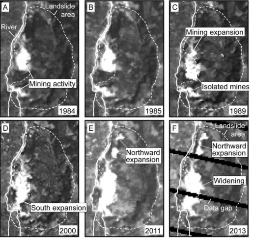
Landsat images from the Global Land Cover Facility (GLCF) catalogue were used to trace the development of the mining activity. We selected cloud-free images from the 30 yr catalogue. We used Landsat TM band 7, i.e., short-wave infrared (2090–

15

2350 nm) for Landsat 4–5 (TM), as shown in Fig. 2a–c, e, and Landsat 7 (ETM+), as shown in Fig. 2d, f, with 30 m resolution. The spectral reflectance of dry soil or sand increases with wavelength and peaks at wavelength 2000–2200 nm (Chudnovsky and Ben-Dor, 2008). Therefore, sand is highly visible in band 7. Band 7 is also sensitive to the moisture content of the soil and vegetation. Moreover, the area of interest was

20

analysed using aerial photographs with pixel resolution∼0.6 m that were recorded in

2007, at the beginning of our InSAR data set. We also studied geological (Edilashvili et al., 1974), land cover and topographic maps (scale 1 : 5000, 1972).

An ASTER DEM (resolution 30 m) was used for morphology analysis and InSAR pro-cessing. We also tested a Shuttle Radar Topography Mission (SRTM) DEM (resolution

25

of 1 and 3 arc-seconds), which did not change our results.

(9)

NHESSD

1, 4925–4962, 2013

InSAR

E. Nikolaeva et. al

Title Page

Tables Figures

◭ ◮

Back Close

Full Screen / Esc

Discussion

P

a

per

|

D

iscussion

P

a

per

|

Discussion

P

a

per

|

Discuss

ion

P

a

per

|

newly formed cracks hidden by vegetation, mapped and measured them with handheld GPS units, and compared them to the InSAR and aerial photography database.

3.2 InSAR

The SAR interferometry (InSAR) method is the complex multiplication of two radar images of the same ground target (Hanssen, 2001). Each radar image contains

ampli-5

tude and phase information. The interferogram is calculated by differencing the phase component of the two coregistered radar images.

To start the interferometric analysis, we coregistered all SAR images to the image acquired at 4 September 2009. Thus, each pixel in all images corresponds to the same location on the ground. Raw images from the FBD mode (14 MHz) were transformed

10

to an FBS mode spacing (28 MHz) using the ROI_PAC (Repeat Orbit Interferometry Package) software. Using DORIS (the Delft Object Oriented Interferometric Software) software (Kampes and Usai, 1999), we built interferograms that contain the phase infor-mation for each acquisition. The effect of topography was calculated and removed from each interferogram using the ASTER DEM with resolution 1 s and satellite ephemeris

15

data (Hanssen, 2001). We generated multi-look images from interferograms with a fac-tor of 2. The multi-looking is necessary to equalise resolution in the azimuthal and in range directions. Therefore, the pixel dimensions are approximately 9 m in the az-imuthal direction and approximately 7.5 m in the range direction. The interferograms were low-pass filtered using adaptive spectral filtering (Principe et al., 2004). The

corre-20

sponding wrapped phase values were unwrapped using the branch-cut phase unwrap-ping algorithm (Goldstein and Werner, 1998) and SNAPHU, a statistical-cost network-flow algorithm (Chen and Zebker, 2002). To correct for the effect of orbital error, wavelet multi-resolution analysis and robust regression were used (Shirzaei and Walter, 2011). Some of the limitations of the InSAR method are related to geometric distortion, for

25

(10)

NHESSD

1, 4925–4962, 2013

InSAR

E. Nikolaeva et. al

Title Page

Tables Figures

◭ ◮

Back Close

Full Screen / Esc

Discussion

P

a

per

|

D

iscussion

P

a

per

|

Discussion

P

a

per

|

Discuss

ion

P

a

per

|

vectors because we did not have access to both ascending and descending tracks (Delacourt et al., 2007). Having only one viewing geometry prohibits the extraction of the 3-D displacement and may affect the interpretation of the deformation field.

3.3 Photographic analysis

The optical data of photographs were transferred to the WGS84 reference frame and

5

analysed in Geographical Information System (GIS) using ArcMap’s Editor Functions. Only one image was available; thus the analysis concentrated on lineaments. This includes manual delineation and classification of lineaments, fractures, streams and ponds. We used the aerial photography in close comparison to the InSAR data. Specif-ically, fractures and morphologic expressions in the aerial photography were compared

10

to changes in the displacement field derived from the InSAR data. This comparison allowed us to test which fractures were active and which were not. The contour map of the area was created from an ASTER 30 m DEM in ArcMap, using 3-D Analyst Tools. The area and perimeter of the landslide boundary were further analysed in ArcMap.

Photography taken by a geotagging camera allowed an even closer view of the

se-15

lected structures and their comparison to InSAR data.

A larger view was possible due to Landsat imagery. After importing these image data to ArcGIS, we were able to visualise the growing extent of the mining activity and its e_ffect on the displacement field.

3.4 Modelling

20

The sliding planes of a landslide play an important role in the activity of the landslide (Petley et al., 2002, 2005). Knowledge of the location, shape and the size of the slid-ing plane allows estimation of the landslide volume. To investigate the geometry of the sliding plane of the observed displacement, we applied inverse modelling techniques. Displacement maps produced from the InSAR data were used as input data. We follow

25

(11)

NHESSD

1, 4925–4962, 2013

InSAR

E. Nikolaeva et. al

Title Page

Tables Figures

◭ ◮

Back Close

Full Screen / Esc

Discussion

P

a

per

|

D

iscussion

P

a

per

|

Discussion

P

a

per

|

Discuss

ion

P

a

per

|

dislocation plane as a first-order approximation (Okada, 1985) of the landslide decolle-ment. The dislocation plane we used has 7 unknowns: length, width, two-dimensional position, dip and strike angles, and dip-slip dislocation components. We used the ge-netic algorithm to search the model and optimise the free parameters (Shirzaei and Walter, 2009), choosing a wide range of possible solutions for the model parameters

5

as a starting point. The genetic algorithm defines a cost function and initialises the genetic algorithm’s parameters.

We used this type of model because large landslides have structures similar to tec-tonic faults (Fleming and Johnson, 1989). Structures found inside a landslide (Fleming and Johnson, 1989) also motivated consideration of dislocation planes in translational

10

landslide rupture models (Fruneau et al., 1996; Muller and Martel, 2000). We follow these previous works by assuming that our observed displacement fields from InSAR may be simulated by planar dislocations within an isotropic elastic half-space. All InSAR deformation measurements were inverted to test the stability of the decollement plane. Only model parameters that emerged when the genetic algorithm had stabilised, which

15

means that the parameters had not changed for several iterations, were considered.

3.5 Estimation of landslide volume

A common way to calculate the rotational landslide volume is to assume that the soil mass has the shape of an ellipsoid (Cruden and Varnes, 1996; Marchesini et al., 2008). We expand on this concept by considering a more complex and realistic landslide

ge-20

ometry: one containing both rotational and translational components. A translational component is considered by considering an ellipsoid segment constrained by two par-allel planes (Fig. 3). The lower plane is the decollement as inverted from our InSAR data, and the upper plane reflects the surface expression of the landslide (Fig. 3). There are two semi-major axes,AandB. Consider the ellipsoid segment with

decolle-25

(12)

NHESSD

1, 4925–4962, 2013

InSAR

E. Nikolaeva et. al

Title Page

Tables Figures

◭ ◮

Back Close

Full Screen / Esc

Discussion

P

a

per

|

D

iscussion

P

a

per

|

Discussion

P

a

per

|

Discuss

ion

P

a

per

|

calculated as follows:

a=A·

q

(1−(h/C)2) (1)

whereais the axis of the ellipse formed by a section planez=h. Then, we are able to calculate the volume of the ellipsoid segment, which is constrained by the two dipping planes:

5

V=

h

Z

0

π·A·B· 1− z

2

C2

!

dz=π·A·B·(h− h

3

3·C2

) (2)

An alternative way to evaluate the volume of a translational or rotational landslide is based on the landslide erosion rate (Hovius et al., 1997; Malamud et al., 2004; Larsen et al., 2010), where the predicted volumeV of a landslide of area S can be approxi-mated by the following empirical relation:

10

V=0.05·S1.3 (3)

The parameter 0.05 was determined empirically for soil landslides (Larsen et al., 2010). An exponent in the range of 1.1–1.3 characterises a soil landslide (Edilashvili et al., 1974), similar to our case in Georgia.

The flow chart (Fig. 3) shows the steps that allow evaluating landslide volumes using

15

the above-described methods.

4 Results

4.1 InSAR deformation field

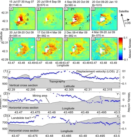
Figure 4 shows the unwrapped and geocoded versions of the InSAR data set. The warm colours (positive values) indicate motion towards the satellite, while cold colours

20

(13)

NHESSD

1, 4925–4962, 2013

InSAR

E. Nikolaeva et. al

Title Page

Tables Figures

◭ ◮

Back Close

Full Screen / Esc

Discussion

P

a

per

|

D

iscussion

P

a

per

|

Discussion

P

a

per

|

Discuss

ion

P

a

per

|

We found the surface pattern of the deformation area to be roughly kidney shaped, where the major axis is approximately north-south parallel to the slope. The landslide is hence approximately 2 km long (north-south) and 0.6 km wide (east-west). A similar pattern emerges from all interferograms, which confirms the displacement occurrence. However, the amplitude of the displacement varies, occasionally even if the same

du-5

ration is bracketed by the data (Fig. 4(1, 2, 3)). This observation complicates the study because the landslide process is found to be highly non-linear. The displacement veloc-ity sharply increases in the interferogram from 4 September 2009–20 October 2009 and extends to almost the entire kidney-shaped landslide surface. The maximum difference between interferograms from 4 September 2009–20 October 2009 and 20 July 2009–

10

4 September 2009 reaches 5 cm. We will provide more information about the possible reasons for different amplitudes in the discussion section.

Three profiles taken from one of the InSAR images (Fig. 4(1, 2, 3)) clearly indicate that no displacement was observed outside the landslide. The bulk of the landslide moves at similar rates, except that sharp gradients can be observed in the toe region.

15

The gaps (Fig. 4(2)) indicate areas of mining activity, where no data are presented due to mining activity, steep topography or erosion.

4.2 Comparison of InSAR to optical images

The surface of the landslide is hummocky and fissured. We found several local pro-trusions and depressions on the landslide body, which were also clear from the profile

20

(Fig. 4(1–3)).

We tested for correlation between the InSAR results and aerial photography (Fig. 5). In most cases, the displacement signals show a strong gradient within the activity zones of the landslide (Fig. 5b–e). Figure 5b shows active graben structures close to the areas of mining activity. Accordingly, these places show displacement gradients.

Fig-25

(14)

NHESSD

1, 4925–4962, 2013

InSAR

E. Nikolaeva et. al

Title Page

Tables Figures

◭ ◮

Back Close

Full Screen / Esc

Discussion

P

a

per

|

D

iscussion

P

a

per

|

Discussion

P

a

per

|

Discuss

ion

P

a

per

|

The geomorphology is complex in case E of Fig. 5: the river path and the shape of topographic isolines suggest that the area was not part of the landslide. However, the displacement signal is similar to the signal on the landslide (Fig. 5e). This observation may suggest that the area was in fact part of the landslide. The gradient visible in the In-SAR data correlates with transverse ridges, possibly associated with the landslide toe.

5

Figure 5f presents an area where fault structures were observed in the field. However, the InSAR result does not show a significant displacement gradient, possibly indicating that the faults had not been active during the InSAR survey. The interferograms sug-gest that these and some of the fault areas are stable (Fig. 5a, f). It is likely that these landslide structures have either very low or no activity, or that any activity is masked by

10

the high density of vegetation. These landslide structures are shown in both Fig. 5 and the survey photographs (Fig. 6).

Because the InSAR data were available only in ascending orbits, a reconstruction of the absolute horizontal and vertical components of the displacement was not possible. We assume, however, that most of the motion is westward because the morphology

15

displays a slope orientation to the west (Fig. 6a). At localised regions, significant ground movement is detected at sites with slopes facing east, thus in the opposite direction. The observation that the movement is affecting both westward- and eastward-facing slopes may lead us to speculate that the type of movement is relatively deep seated and involves both synthetic and antithetic faults (Fig. 6b) to form horst and graben

20

structures. In other words, local morphologic features (Fig. 6c, d) and slopes have only minor influence on the moving mass, which is controlled instead by the large-scale topography and a deep-seated decollement.

Due to the slow rate of the landslide, the surface activity of the sliding area is not clear in optical Landsat satellite imagery (Fig. 2). Investigation of high-resolution aerial

25

(15)

NHESSD

1, 4925–4962, 2013

InSAR

E. Nikolaeva et. al

Title Page

Tables Figures

◭ ◮

Back Close

Full Screen / Esc

Discussion

P

a

per

|

D

iscussion

P

a

per

|

Discussion

P

a

per

|

Discuss

ion

P

a

per

|

We created a sketch of the landslide in GIS, using aerial and InSAR results as well as field observations (Fig. 7). We identified partly water-filled ponds in the transition zone of the centre to the upper part of the landslide (Fig. 7). Although the ponds and boggy areas are morphologically well explained, they were not present on the 1972 topo-graphic map, implying that they developed more recently. Furthermore, some houses

5

were built in locations where ponds are located today, for instance, close to the eastern slope (latitude 42.2975◦_{N, longitude 43.488}◦_{E). In the field, we identified trees or their}

remnants inside the ponds, which supports the idea that the ponds have appeared recently.

We identified visible scarps for this region from the aerial photograph and field

ob-10

servations (Fig. 7). The major areas of debris are on the eastern slope of the landslide. Over the course of our field season, the debris flow tracks, debris fan deposits and scars evolved. Newly formed cracks hidden by vegetation were found during field sur-veying.

The area affected by landslide processes was calculated in GIS using a polygon

cre-15

ated based on InSAR, aerial photography and field observations (Fig. 7). We found that the area of the kidney-shaped landslide identified by its morphology is approximately 2.9 km2, the perimeter of total area affected by the landslide is approximately 7.48 km, and the area having a displacement signal from InSAR is approximately 0.9 km2.

4.3 Modelling results

20

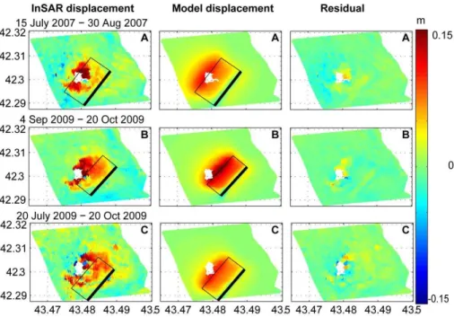
We inverted the three best interferograms with temporal baselines of 46 or 90 days. Fig-ure 8 shows the observed displacements from InSAR data, model simulations of the same geometry and residuals that show the difference between those two displace-ment fields. In all these datasets, the optimum decolledisplace-ment plane is sub-horizontal and dips slightly to the northwest. The residuals are generally less than 5 cm, which

25

(16)

NHESSD

1, 4925–4962, 2013

InSAR

E. Nikolaeva et. al

Title Page

Tables Figures

◭ ◮

Back Close

Full Screen / Esc

Discussion

P

a

per

|

D

iscussion

P

a

per

|

Discussion

P

a

per

|

Discuss

ion

P

a

per

|

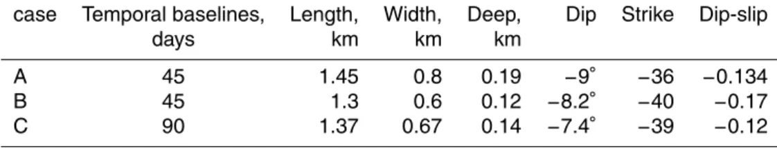
We detected a slight variation of the location and geometry of the sliding plane. For example, the dip ranges between−2◦ and −12◦ westward, the strike ranges between

35◦_{and 45}◦_{northeast-southwest, the dip slip ranges between}

−0.15 m and−0.25 m to

the northwest and the depth ranges from 120 m to 190 m below the surface. As these inversions provide an indirect view on the decollement plane, we can now elaborate on

5

the landslide volume.

4.4 Landslide volume

Using the ellipsoid segment concept, we calculated the geometrically predicted volume based on the surface affected and the location of the decollement plane. We present displacement on the surface as an ellipse with semi-major axesA andB, which have

10

values of 0.3 km and 1 km, respectively (Fig. 3). The axisAis found from modelling as the length parameter (average 0.65 km) andhis the modelled depth of the detachment plane (average 0.12 km). Based on these parameters and using Eq. (2), we estimated the volume of the Itskisi landslide to be 0.09 km2. We did not include dip in our volume estimation because the slope of the target area is approximately 10◦_{, which is similar} 15

to the dip angle of the decollement as obtained from inverse modelling.

Following the empirical Eq. (3) and using the affected landslide area as determined from InSAR, we obtain a landslide volume of approximately 0.046 km3, which is half the volume estimated above. Several reasons may explain this difference. Firstly, we do not take the slope of the planes that are truncated ellipsoids into account. Secondly, the

20

(17)

NHESSD

1, 4925–4962, 2013

InSAR

E. Nikolaeva et. al

Title Page

Tables Figures

◭ ◮

Back Close

Full Screen / Esc

Discussion

P

a

per

|

D

iscussion

P

a

per

|

Discussion

P

a

per

|

Discuss

ion

P

a

per

|

5 Discussion

We use both InSAR and optical data for the detection and kinematic analysis of a land-slide in Georgia. The landland-slide is 0.9 km3 in area, subject to a motion of up to 6 cm within 46 days and a_ffects a populated region and a major mining site. Although we use radar data from a single direction (ascending satellite pass) only, the combination

5

of InSAR displacement maps, aerial photography analysis and modelling provides in-formation about the landslide dynamics. One of the important problems that may be encountered in the processing of radar images is the loss of coherence due to spa-tial or temporal factors. For this reason, we excluded some interferograms from our analysis and modelling. In the following section, we discuss the effects of extrinsic

pro-10

cesses, such as those related to rainfall, earthquake and mining activity, on landslide dynamics.

5.1 Impacts

The landslide may affect surrounding infrastructure, population and river flow. Land-slides can dam rivers (Fig. 7), which may induce major hydrological hazards such as

15

floods or the loss of drinking water resources. Landslides also affect erosion and can cause term losses of topsoil and vegetation. Landslide damming has both short-and long-term effects (Schuster and Highland, 2003). The Itskisi landslide directly af-fected four villages: Itskisi, Makhatauri, Savane and Irtavaza (Fig. 10). The village of Itskisi is located directly on the landslide and moved downslope. Houses there were

20

(18)

NHESSD

1, 4925–4962, 2013

InSAR

E. Nikolaeva et. al

Title Page

Tables Figures

◭ ◮

Back Close

Full Screen / Esc

Discussion

P

a

per

|

D

iscussion

P

a

per

|

Discussion

P

a

per

|

Discuss

ion

P

a

per

|

5.2 Factors triggering landslides

A displacement signal is detected in each interferogram shown in Fig. 4 and is partic-ularly strong in interferograms with short temporal baselines. Because variation in the displacement rates a_ffects only the kidney-shaped landslide area and not the stable surroundings, we conjecture that this variation is not an artefact. The normalised

ve-5

locity value suggests highly variable slip rates. The changes in the velocity may be due to variations in groundwater, which are a function of rainfall intensity or seasonal water variations such as snowmelt.

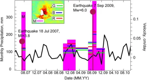
We select the average velocity at four different places on the landslide (Fig. 4a–h) to investigate the relationship between changes in velocity and precipitation. We

com-10

pare these velocities to average monthly precipitation data (Fig. 9 black curve), which is based on the atmospheric general circulation model ECHAM5 (http://www.mpimet. mpg.de). The period from June 2007 to January 2010 has a maximum precipitation value of 150 mm. The interferograms from 17 October 2008–4 March 2009, 2 Decem-ber 2008–4 March 2009 and 20 OctoDecem-ber 2009–20 January 2010 (Fig. 4) cover periods

15

with monthly precipitation below 150 mm, while all other interferograms cover intervals with monthly precipitation less than 100 mm. The velocity in the interferogram from 2 December 2008–4 March 2009 is slightly higher (0.01 cm day−1_{) than in the}

interfer-ogram from 4 March 2009–20 July 2009. However, we observe that the interferinterfer-ograms with higher velocities tend to occur close to the dates of minimum monthly average

20

precipitation (Fig. 9). These interferograms cover the time from 20 July 2009–20 Oc-tober 2009 and 15 July 2007–30 August 2007. Thus, the apparent acceleration of the landslide in September–October 2009 cannot be explained by rainfall.

Inspection of the global earthquake catalogue (CMT) shows that a magnitude Mw=6.0 earthquake on 7 September 2009 occurred at 10 km depth and a distance of

25

(19)

NHESSD

1, 4925–4962, 2013

InSAR

E. Nikolaeva et. al

Title Page

Tables Figures

◭ ◮

Back Close

Full Screen / Esc

Discussion

P

a

per

|

D

iscussion

P

a

per

|

Discussion

P

a

per

|

Discuss

ion

P

a

per

|

suggests that these earthquakes may have had a triggering influence. This is in agree-ment with work by Jibson et al. (1994), where numerous landslides were triggered following an earthquake at a distance of approximately 30 km.

These discussions are relevant given the on-going mining activity during the period of this study. There is 68.07 Ha of mining area covered by 17 mining companies (source:

5

www.gwp.org, licenses issued for the use of mineral resources in Georgia), as shown in Fig. 2 (bright areas). These images do not allow clear analysis of the landslide, but they do show the development of mining activity (Fig. 2, bright areas). Quartz sand extraction began in 1968 and accelerated greatly in 2007, reaching rates that continue today. This may explain why the points closest to the active mines show the highest

10

velocities in 2007 (Fig. 9, margin line, year 2007).

We conclude that the landslide may have been triggered by rainfall, earthquakes and the man-made removal of the toe. Unfortunately, due to the lack of good topo-graphic data, ground data and field information at that time, no clear relation between the earthquakes and the triggering of the landslide movements could be found.

15

5.3 Conceptual model

Our structural mapping and analysis of InSAR data suggest that several smaller sliding blocks combine to form the larger landslide complex. We applied a model to study the internal geometry of the landslide.

Inspired by the research of Fleming and Johnson (1989), Muller and Martel (2000)

20

and Martel (2004), we use a dislocation model to evaluate the depth of the sliding plane. The hypothesis is that the structures of large landslides are similar to tectonic faults. For instance, the seismic and geodetic observations confirmed analogous behaviour of landslide detachment planes and tectonic faults (Gomberg and Bodin, 1995). More-over, the geometry of these two elements may also be related, as was found between

25

(20)

NHESSD

1, 4925–4962, 2013

InSAR

E. Nikolaeva et. al

Title Page

Tables Figures

◭ ◮

Back Close

Full Screen / Esc

Discussion

P

a

per

|

D

iscussion

P

a

per

|

Discussion

P

a

per

|

Discuss

ion

P

a

per

|

may play important roles in the development of the landslide process. We did not con-sider possible material heterogeneity, nor did we take into account topography or the distributions of possible driving forces and gravitation. Our model also does not show the evolution of a landslide and secondary slides and has difficulty predicting the true shape of the sliding plane. However, in the first approximation, the model selects the

5

potential sliding plane most susceptible to failure from an infinite number of potential surfaces. In addition, translational slides can be connected to upslope and downslope rotational slides (Fig. 10). The lengths of the displacement vectors remain the same at certain areas (Fig. 10, profile), and the distribution of the displacement vectors is a function of the slip-surface sliding plane (Casson et al., 2005). The equal displacement

10

vectors in the centre zone of the landslide indicate a uniform translational landslide there (Casson et al., 2005). However, the lengths of the displacement vectors increase from east to west, which implies the presence of rotational landslide elements in the upper zone (Fig. 10, profile).

The complete picture of the landslide therefore consists of a planar (translational)

15

fault at depth that curved toward the toe and headwall to form a combined rotational-translational landslide body. Secondary landslides developed and migrated, piggyback-ing on each other. Antithetic faults and horst and graben structures developed. The grabens formed ponds and destroyed the Itskisi village, whereas the horst structures are currently exploited by mining activity. A local girdle of subsidence surrounding the

20

mine highlights the effects of the loss of toe support. Landslides may be triggered by mining intensification (as in 2007) or earthquakes (as in 2009). A direct link to rainfall was not found, though we note that the rainfall database was poor.

Previous studies show the efficiency of combining different remote sensing images for monitoring and characterising landslide processes (Casson et al., 2005; Strozzi et

25

(21)

NHESSD

1, 4925–4962, 2013

InSAR

E. Nikolaeva et. al

Title Page

Tables Figures

◭ ◮

Back Close

Full Screen / Esc

Discussion

P

a

per

|

D

iscussion

P

a

per

|

Discussion

P

a

per

|

Discuss

ion

P

a

per

|

(Casson et al., 2005). The aim of the conceptual model is the evaluation of the volume of possible landslides for the hazard mass movement.

6 Conclusions and perspective

Landslides in the area of the Caucasus Mountains are not well monitored due to the high costs and difficult logistics of doing so. As we demonstrate, the combination of

5

InSAR data, aerial photography analysis, Landsat imagery and other information allows us to identify and monitor a landslide in the centre part of Georgia. The displacement rate of the landslide is from 10 cm yr−1_{to 30 cm yr}−1_{, covering an area of approximately}

0.9 km2. We analysed the activity of a landslide over a five-year period. We find that the landslide is conditionally faster and discuss potential external triggers.

10

We characterise landslide movements and determine displacement velocities within the landslide bodies. By combining this work with modelling, we are able to more pre-cisely explore the dimensions and detachment plane geometry and further illuminate potential hazards and environmental interactions. The maximum depth of the landslide detachment plane ranges from 0.12 km to 0.19 km.

15

Field observations show good correlation of surface fractures and the displacements obtained from InSAR data (Fig. 5 and Fig. 6). We identify a number of factors that may trigger landslides. Mining caused a loss of mass in the toe. The intensification of min-ing exploration locally increased the landslide velocity. In addition, the most dramatic velocity increase was found in association with aMw=6.0 earthquake located 30 km

20

from the landslide.

This landslide poses threats to human lives and structures that support transporta-tion and natural resource management in four villages. The danger of a landslide is that earthquakes can cause it to suddenly become catastrophic. This finding has im-portant implications for hazard assessment because the location and type of landslides

25

(22)

NHESSD

1, 4925–4962, 2013

InSAR

E. Nikolaeva et. al

Title Page

Tables Figures

◭ ◮

Back Close

Full Screen / Esc

Discussion

P

a

per

|

D

iscussion

P

a

per

|

Discussion

P

a

per

|

Discuss

ion

P

a

per

|

Over the past 30 yr, the use of remote sensing techniques in the geosciences has increased dramatically. The number of satellites with various temporal and spatial res-olutions, bands and broad coverage has also increased. In this regard, there is greater opportunity to explore an event with various datasets. The probability of data being available for unexpected geological disasters is also higher. This remote sensing

devel-5

opment plays a major role for creating a data archive for Georgia, where high hazards exist but only small numbers of observational tools are used.

The results of this study demonstrate that complex remote sensing techniques have the potential to become good tools for early warning of landslide disasters. Satellite data allow monitoring landslides in space and time. The displacement distribution

ob-10

tained from InSAR data can be used in a model to characterise the geometry and spatial evolution of the landslide slip surface. Its temporal evolution can also be inves-tigated with remote sensing data.

Acknowledgements. Elena Nikolaeva would like to thank the DAAD (German Academic

Exchange Service)for financially supporting the PhD research of Elena Nikolaeva, theInstitute

15

ofEarth Sciencesat Ilia State Universityin Tbilisi (Georgia) for organisation of field work and providing aerial photographs, Henriette Sudhaus and Hannes Bathke for their valuable advice during the processing of radar data and Michele Pantaleo for geology discussions.

The service charges for this open access publication 20

have been covered by a Research Centre of the Helmholtz Association.

References

Canuti, P., Casagli, N., Catani, F., Falorni, G., and Farina, P.: : Integration of Remote Sensing Techniques, in: Different Stages of Landslide Response, Progress in Landslide, Science, 25

251–260, 2007.

(23)

mon-NHESSD

1, 4925–4962, 2013

InSAR

E. Nikolaeva et. al

Title Page

Tables Figures

◭ ◮

Back Close

Full Screen / Esc

Discussion

P

a

per

|

D

iscussion

P

a

per

|

Discussion

P

a

per

|

Discuss

ion

P

a

per

|

itoring. The International Archives Of The Photogrammetry, Remote Sensing And Spatial Information Sciences XXXVII, 235–240, 2001.

Casson, B., Delacourt, C., and Allemand, P.: Contribution of multi-temporal remote sensing im-ages to characterize landslide slip surface - Application to the La Clapière landslide (France), Nat. Hazards Earth Syst. Sci., 5, 425–437, doi:10.5194/nhess-5-425-2005, 2005.

5

Chen, C., Zhang, J., and Lu, L.: Identification of Layover and Shadow Regions in InSAR Image, 2011 International Symposium on Image and Data Fusion, IEEE, 1–4, 2011.

Chen, C. W. and Zebker, H. A.: Phase unwrapping for large SAR interferograms: statistical segmentation and generalized network models, IEEE T. Geosci. Remote, 40, 1709–1719, doi:10.1109/TGRS.2002.802453, 2002.

10

Chudnovsky, A. and Ben-Dor, E.: Application of visible, near-infrared, and short-wave infrared (400–2500 nm) reflectance spectroscopy in quantitatively assessing settled dust in the indoor environment, Case study in dwellings and o_ffice environments, Sci. Total Environ., 393, 198– 213, doi:10.1016/j.scitotenv.2007.11.022, 2008.

Colesanti, C., Ferretti, A., Prati, C., and Rocca, F.: Monitoring landslides and tectonic mo-15

tions with the Permanent Scatterers Technique, Eng. Geol., 68, 3–14, doi:10.1016/S0013-7952(02)00195-3, 2003.

Colesanti, C. and Wasowski, J.: Investigating landslides with space-borne Synthetic Aperture Radar (SAR) interferometry, Eng. Geol., 88, 173–199, doi:10.1016/j.enggeo.2006.09.013, 2006.

20

Cruden, D. M.: The geometry of slip surfaces beneath landslides: predictions from surface measurements: Discussion, Can. Geotech. J., 23, 94, doi:10.1139/t86-012, 1986.

Cruden, D. M. and Varnes, D. J.: Landslide types and processes, in: Landslides – Investigation and Mitigation, edited by: Turner, A. T. and Schuster, R. L., Trans. Res. B., 247, 36–75, doi:10.1007/BF02590167, 1996.

25

Delacourt, C., Allemand, P., Berthier, E., Raucoules, D., Casson, B., Grandjean, P., Pambrun, C., and Varel, E.: Remote-sensing techniques for analysing landslide kinematics: a review, B. Soc. Geol. Fr., 178, 89–100, doi:10.2113/gssgfbull.178.2.89, 2007.

Edilashvili, V. Y., Lekvinadze, R. D., and Gogiberidze, V. V.: E_ffect of tectonics on manganese accumulation in Georgia, Int. Geol. Rev., 16, 439–445, doi:10.1080/00206817409471856, 30

1997.

(24)

NHESSD

1, 4925–4962, 2013

InSAR

E. Nikolaeva et. al

Title Page

Tables Figures

◭ ◮

Back Close

Full Screen / Esc

Discussion

P

a

per

|

D

iscussion

P

a

per

|

Discussion

P

a

per

|

Discuss

ion

P

a

per

|

Fruneau, B., Achache, J., and Delacourt, C.: Observation and modelling of the Saint-Étienne-de-Tinée landslide using SAR interferometry, Tectonophysics, 265, 181–190, doi:10.1016/S0040-1951(96)00047-9, 1996.

Gamkrelidze, I. and Shengelia, D.: Pre-Alpine Geodynamics of the caucasus, Suprasubduction Regional Metamorphism and Granitoid Magmatism, Bull. of Georgian National Acad. of Sci., 5

175, 57–65, 2007.

García-Davalillo, J. C., Herrera, G., Notti, D., Strozzi, T., and Álvarez-Fernández, I.: DInSAR analysis of ALOS PALSAR images for the assessment of very slow landslides: the Tena Valley case study, Landslides, doi:10.1007/s10346-012-0379-8, 2013.

Goldstein, R. M. and Werner, C. L.: Radar interferogram filtering for geophysical applications, 10

Geophys. Res. Lett., 25, 4035–4038, doi:10.1029/1998GL900033, 1998.

Gomberg, J. and Bodin, P.: Landslide faults and tectonic faults, analogs: The Slumgullion earth-flow, Colorado, Geology, 23, 41, doi:10.1130/0091-7613(1995)023<0041:LFATFA>2.3.CO;2, 1995.

Gracheva, R. and Golyeva, A.: Landslides in mountain regions: hazards, resources and in-15

formation, in: Geophysical Hazards, International Year of Planet Earth, edited by: Beer, T., Geophysical Hazards, Springer Netherlands, Dordrecht, 249–260, 2010.

Guzzetti, F., Manunta, M., Ardizzone, F., Pepe, A., Cardinali, M., Zeni, G., Reichenbach, P., and Lanari, R.: Analysis of Ground Deformation Detected Using the SBAS-DInSAR Technique in Umbria, Central Italy, Pure Appl. Geophys., 166, 1425–1459, doi:10.1007/s00024-009-0491-20

4, 2009.

Guzzetti, F., Mondini, A. C., Cardinali, M., Fiorucci, F., Santangelo, M., and Chang, K. T.: Landslide inventory maps: New tools for an old problem, Earth-Sci. Rev., 112, 42–66, doi:10.1016/j.earscirev.2012.02.001, 2012.

Hanssen, R. F.: Radar Interferometry: Data Interpretation and Error Analysis, Springer, 328, 25

2001.

Highland, L. M. and Bobrowsky, P.: The Landslide Handbook – A Guide to Understanding, Landslides, Geological Survey Circular, 1325, 129, 2008.

Hilley, G. E., Bürgmann, R., Ferretti, A., Novali, F., and Rocca, F.: Dynamics of slow-moving landslides from permanent scatterer analysis, Science (New York, NY), 304, 1952–1955, 30

(25)

NHESSD

1, 4925–4962, 2013

InSAR

E. Nikolaeva et. al

Title Page

Tables Figures

◭ ◮

Back Close

Full Screen / Esc

Discussion

P

a

per

|

D

iscussion

P

a

per

|

Discussion

P

a

per

|

Discuss

ion

P

a

per

|

Hovius, N., Stark, C. P., and Allen, P. A.: Sediment flux from a mountain belt derived by landslide mapping, Geology, 25, 231–234, doi:10.1130/0091-7613(1997)025<0231:SFFAMB>2.3.CO;2, 1997.

Iverson, R. M., Reid, M. E., Iverson, N. R., La Husen, R. G., Logan, M., Mann, J. E., and Brien, D. L.: Acute Sensitivity of Landslide Rates to Initial Soil Porosity, Science, 290, 513–516, 5

doi:10.1126/science.290.5491.513, 2000.

Jaboyedoff, M., Oppikofer, T., Abellán, A., Derron, M.-H., Loye, A., Metzger, R., and Pe-drazzini, A.: Use of LIDAR in landslide investigations: a review, Nat. Hazards, 61, 5–28, doi:10.1007/s11069-010-9634-2, 2010.

Jibson, R. W., Prentice, C. S., Borissoff, B. A., Rogozhin, E. A., and Langeret, C. J.: Some 10

observations of landslides triggered by the 29 April 1991 Racha earthquake, Republic of Georgia, B. Seismol. Soc. Am., 84, 963–973, 1994.

Kampes, B. and Usai, S.: Doris: The Delft object-oriented radar interferometric software, 2nd International Symposium on Operationalization of Remote Sensing, Enschede, The Nether-lands, Citeseer, p. 20, 1999.

15

Larsen, I. J., Montgomery, D. R., and Korup, O.: Landslide erosion controlled by hillslope mate-rial, Nat. Geosci. 3, 247–251, doi:10.1038/ngeo776, 2010.

Leonov, M. G.: Fractures in the Dzirula massif (Georgia), Int. Geol. Rev., 18, 1019–1024, doi:10.1080/00206817609471311, 1976.

Malamud, B. D., Turcotte, D. L., Guzzetti, F., and Reichenbach, P.: Landslide inventories and 20

their statistical properties, Earth. Surf. Proc. Land., 29, 687–711, doi:10.1002/esp.1064, 2004.

Martel, S.: Mechanics of landslide initiation as a shear fracture phenomenon, Mar. Geol., 203, 319–339, doi:10.1016/S0025-3227(03)00313-X, 2004.

Martha, T. R., Kerle, N., Jetten, V., van Westen, C. J., and Kumar, K. V.: Characterising spectral, 25

spatial and morphometric properties of landslides for semi-automatic detection using object-oriented methods, Geomorphology, 116, 24–36, doi:10.1016/j.geomorph.2009.10.004, 2010.

Muller, J. R. and Martel, S. J.: Numerical Models of Translational Landslide Rupture Surface Growth, Pure Appl. Geophys., 157, 1009–1038, doi:10.1007/s000240050015, 2000.

30

(26)

NHESSD

1, 4925–4962, 2013

InSAR

E. Nikolaeva et. al

Title Page

Tables Figures

◭ ◮

Back Close

Full Screen / Esc

Discussion

P

a

per

|

D

iscussion

P

a

per

|

Discussion

P

a

per

|

Discuss

ion

P

a

per

|

Nichol, J. and Wong, M. S.: Satellite remote sensing for detailed landslide invento-ries using change detection and image fusion, Int. J. Remote Sens., 26, 1913–1926, doi:10.1080/01431160512331314047, 2005.

Okada, Y.: Surface deformation due to shear and tensile faults in a half-space, B. Seismol. Soc. Am., 75, 1135–1154, doi:10.1016/0148-9062(86)90674-1, 1985.

5

Ouimet, W. B.: Landslides associated with the May 12, 2008 Wenchuan earthquake: Implica-tions for the erosion and tectonic evolution of the Longmen Shan, Tectonophysics, 491, 244– 252, doi:10.1016/j.tecto.2009.09.012, 2010.

Perski, Z., Hanssen, R., Wojcik, A., and Wojciechowski, T.: InSAR analyses of ter-rain deformation near the Wieliczka Salt Mine, Poland, Eng. Geol., 106, 58–67, 10

doi:10.1016/j.enggeo.2009.02.014, 2009.

Petley, D. N., Bulmer, M. H., and Murphy, W.: Patterns of movement in rotational and transla-tional landslides, Geology, 30, 719–722, 2002.

Petley, D. N., Mantovani, F., Bulmer, M. H. K., and Zannoni, F.: The use of surface monitoring data for the interpretation of landslide movement patterns, Geomorphology, 66, 133–147, 15

2005.

Principe, J. C., De Vries B., and De Oliveira, P. G.: The gamma-filter-a new class of adaptive IIR filters with restricted feedback, IEEE T. Signal Proces., 41, 3378–3393, doi:10.1109/TSP.2004.837406, 2004.

Qi, S., Xu, Q., Lan, H., Zhang, B., and Liu, J.: Spatial distribution analysis of land-20

slides triggered by 2008.5.12 Wenchuan Earthquake, China, Eng. Geol. 116, 95–108, doi:10.1016/j.enggeo.2010.07.011, 2010.

Riedel, B. and Walther, A.: InSAR processing for the recognition of landslides, Adv. Geosci., 14, 189–194, doi:10.5194/adgeo-14-189-2008, 2008.

Sandwell, D. T., Myer, D., Mellors, R., Shimada, M., Brooks, B., and Foster, J.: Accuracy and 25

Resolution of ALOS Interferometry: Vector Deformation Maps of the Father’s Day Intrusion at Kilauea, IEEE T. Geosci. Remote, 46, 3524–3534, doi:10.1109/TGRS.2008.2000634, 2008. Schulz, W. H.: Landslides mapped using LIDAR imagery, Seattle, Washington, U.S. Geological

Survey Open-File Report 2004–1396, 11 pp., 1 plate, 2004.

Schulz, W. H.: Landslide susceptibility revealed by LIDAR imagery and historical records, Seat-30

(27)

NHESSD

1, 4925–4962, 2013

InSAR

E. Nikolaeva et. al

Title Page

Tables Figures

◭ ◮

Back Close

Full Screen / Esc

Discussion

P

a

per

|

D

iscussion

P

a

per

|

Discussion

P

a

per

|

Discuss

ion

P

a

per

|

Schuster, R. L. and Highland, L. M.: Impacts of mass wasting on the natural environment, 2007, Environ. Eng. Geosci., co-published by the Geolgoical Society of America (GSA) and the Association of Engineering Geologists, (AEG), Vol. XIII, No. 1, February, 25–44, 2007. Shirzaei, M. and Walter, T. R.: Randomly iterated search and statistical competency as

pow-erful inversion tools for deformation source modeling: Application to volcano interferometric 5

synthetic aperture radar data, J. Geophys. Res., 114, B10401, doi:10.1029/2008JB006071, 2009.

Shirzaei, M. and Walter, T. R.: Estimating the Effect of Satellite Orbital Error Using Wavelet-Based Robust Regression Applied to InSAR Deformation Data, IEEE T. Geosci. Remote, 49, 4600–4605, doi:10.1007/s11004-009-9234-4, 2011.

10

Strozzi, T., Ambrosi, C., and Raetzo, H.: Interpretation of Aerial Photographs and Satel-lite SAR Interferometry for the Inventory of Landslides, Remote Sensing, 5, 2554–2570, doi:10.3390/rs5052554, 2013.

Strozzi, T., Farina, P., Corsini, A., Ambrosi, C., Thüring, M., Zilger, J., Wiesmann, A., Weg-müller, U., and Werner, C.: Survey and monitoring of landslide displacements by means of 15

L-band satellite SAR interferometry, Landslides, 2, 193–201, doi:10.1007/s10346-005-0003-2, 2005.

Tofani, V., Segoni, S., Agostini, A., Catani, F., and Casagli, N.: Technical Note: Use of re-mote sensing for landslide studies in Europe, Nat. Hazards Earth Syst. Sci., 13, 299–309, doi:10.5194/nhess-13-299-2013, 2013.

20

Van Westen, C. J., Straatsma, M. W., Turdukulov, U. D., et al. (Eds.): Atlas of Natural Hazards and Risk in Georgia. Caucasus Environmental NGO Network (CENN), University of Twente Faculty of Geo-Information and Earth Observation (ITC), ISBN: 978-9941-0-4310-9, (http: //drm.cenn.org/paper_atlas/RA-part-1.pdf), 2012.

Varnes, D. J.: Slope movement types and processes, Landslide analysis and control, National 25

Academy of Sciences, 11–33, 1978.

(28)

NHESSD

1, 4925–4962, 2013

InSAR

E. Nikolaeva et. al

Title Page

Tables Figures

◭ ◮

Back Close

Full Screen / Esc

Discussion

P

a

per

|

D

iscussion

P

a

per

|

Discussion

P

a

per

|

Discuss

ion

P

a

per

|

Table 1.Output parameters from inversion model for different interferograms (Fig. 8a–c).

case Temporal baselines, Length, Width, Deep, Dip Strike Dip-slip

days km km km

(29)

NHESSD

1, 4925–4962, 2013

InSAR

E. Nikolaeva et. al

Title Page

Tables Figures

◭ ◮

Back Close

Full Screen / Esc

Discussion

P

a

per

|

D

iscussion

P

a

per

|

Discussion

P

a

per

|

Discuss

ion

P

a

per

|

Fig. 1.Map of central Georgia showing land cover based on Landsat TM information. The