Variations in leaf physiological properties within Amazon forest canopies

(1)

BGD

6, 4639–4692, 2009

Amazon forest canopies

J. Lloyd et al.

Title Page

Abstract Introduction

Conclusions References

Tables Figures

◭ ◮

Back Close

Full Screen / Esc

Printer-friendly Version

Interactive Discussion

Biogeosciences Discuss., 6, 4639–4692, 2009 www.biogeosciences-discuss.net/6/4639/2009/ © Author(s) 2009. This work is distributed under the Creative Commons Attribution 3.0 License.

Biogeosciences Discussions

Biogeosciences Discussionsis the access reviewed discussion forum ofBiogeosciences

Variations in leaf physiological properties

within Amazon forest canopies

J. Lloyd1, S. Pati ˜no2, R. Q. Paiva3,*, G. B. Nardoto4, C. A. Quesada1,3,5, A. J. B. Santos3,5,†, T. R. Baker1, W. A. Brand6, I. Hilke6, H. Gielmann6, M. Raessler6, F. J. Luiz ˜ao3, L. A. Martinelli4, and L. M. Mercado7

1

Earth and Biosphere Institute, School of Geography, University of Leeds, LS2 9JT, UK 2

Grupo de Ecolog´ıa de Ecosistemas Terrestres Tropicales, Universidad Nacional de

Colombia, Sede Amazonia, Instituto Amaz ´onico de Investigaciones-Imani, km. 2, v´ıa

Tarapac ´a, Leticia, Amazonas, Colombia 3

Institito National de Pesquisas Amaz ˆonicas, Manaus, Brazil 4

Centro de Energia Nuclear na Agricultura, Av. Centen ´ario 303, 13416-000, Piracicaba-SP, Brazil

5

Departamento de Ecologia, Universidade de Bras´_ılia, DF, Brazil

6

Max-Planck-Institut f ¨ur Biogeochemie, Postfach 100164, 07701, Jena, Germany 7

(2)

BGD

6, 4639–4692, 2009

J. Lloyd et al.

Title Page

Tables Figures

◭ ◮

Back Close

Full Screen / Esc

∗

now at: Secret ária Municipal de Desenvolvimento e Meio Ammbiente ma Prefeturia Municipal de Mau és, Mau és, Brazil

†_{Alexandre Santos died in the Amazon plane crash of 29 September 2006}

Received: 18 December 2008 – Accepted: 3 February 2009 – Published: 5 May 2009

Correspondence to: J. Lloyd (j.lloyd@leeds.ac.uk)

(3)

BGD

6, 4639–4692, 2009

J. Lloyd et al.

Title Page

Tables Figures

◭ ◮

Back Close

Full Screen / Esc

Interactive Discussion Abstract

Vertical profiles in leaf mass per unit leaf area (MA), foliar13C composition (δ13C) and

leaf nitrogen (N), phosphorus (P), carbon (C), potassium (K), magnesium (Mg) and cal-cium (Ca) concentrations were estimated for 204 rain forest trees growing in 57 sites across the Amazon Basin. Data was analysed using a multilevel modelling approach,

5

allowing a separation of gradients within individual tree canopies (intra-tree gradients) as opposed to stand level gradients occurring because of systematic differences oc-curring between different trees of different heights (inter-tree gradients). Significant positive intra-tree gradients (i.e. increasing values with increasing sampling height) were observed forM_A and [C]_DW (the subscript denoting on a dry weight basis) with

10

negative intra-tree gradients observed for δ13C, [Mg]_DW and [K]_DW . No significant intra-tree gradients were observed for [N]DW, [P]DW or [Ca]DW. Although the

magni-tudes of inter-tree gradients were not significantly different forM_A,δ13C, [C]_DW, [K]_DW , [N]_DW, [P]_DW and [Ca]_DW , for [Mg]_DW there no systematic difference observed be-tween trees of different heights, this being in contrast to the strongly negative intra-tree

15

gradients also found to exist.

When expressed on a leaf area basis, significant positive gradients were observed for N, P and K both within and between trees, these being attributable to the positive intra-and inter-tree gradients inM_Amentioned above. No systematic intra-tree gradient was observed for either Ca or Mg when expressed on a leaf area basis, but with a significant

20

positive gradient observed for Mg between trees (i.e. with taller trees tending to have a higher Mg per unit area).

In contrast to the other variables measured, significant variations in intra-tree gra-dients for di_fferent individuals were found to exist for MA, δ

13

C and [P] (area basis). This was best associated with the overall average area based [P], this also being

con-25

(4)

non-BGD

6, 4639–4692, 2009

J. Lloyd et al.

Title Page

Tables Figures

◭ ◮

Back Close

Full Screen / Esc

existent gradients inAmax, with optimal intra-canopy gradients becoming sharper as a tree’s upper canopyAmax increases. Nevertheless, in all cases it is predicted that the optimal within-canopy gradients inAmax should be less than is generally observed for photon irradiance. Although this is consistent with numerous observations, it is also in contrast to previously held notions of optimality.

5

1 Introduction

It has long been observed that the light saturated photosynthetic rates of leaves lo-cated low in plant canopies can be typically much less than leaves receiving much more irradiance (Q) higher up (Jarvis et al., 1976) and this has been typically attributed to gradients in foliar nitrogen contents on a leaf area basis (Field, 1983). Nitrogen is

10

a critical component of the photosynthetic apparatus (Evans, 1989) and it been shown that a theoretically optimal distribution of nitrogen concentration maximizes canopy photosynthesis when nitrogen concentrations closely follows the distribution ofQ, ap-proaching zero whenQalso does (Field, 1983; Chen et al., 1993). Nevertheless, one regular observation in tree canopies seems to be that vertical gradients in

photosyn-15

thetic capacity seem to be much less than that which would be optimal to maximise individual plant carbon gain (e.g. Hollinger, 1996; Kull and Niinemets, 1998; Meir et al., 2002; Wright et al., 2006).

Understanding and quantifying within canopy gradients in photosynthetically impor-tant nutrient and associated changes in plant physiological properties is also imporimpor-tant

20

for simulating rates of canopy photosynthesis and the associated light response (Lloyd et al., 1995; Haxeltine and Prentice, 1996; de Pury and Farquhar, 1997) as well as for simulations of canopy leaf areas (themselves affecting predicted rates of photosyn-thetic carbon gain) in dynamic vegetation models (Sitch et al., 2003; Woodward and Loomis, 2004). Within tropical forest canopies, this variation may be expected to be

25

(5)

BGD

6, 4639–4692, 2009

J. Lloyd et al.

Title Page

Tables Figures

◭ ◮

Back Close

Full Screen / Esc

to asymptotic tree height (Lloyd et al., 1995; Thomas and Bazzaz, 1999; Rijkers et al., 2000) successional status (Popma et al., 1992; Reich et al., 1995) and/or shade toler-ance (Turner, 2001). Mean vertical variations in nutrient concentrations and associated physiological characteristics within tropical forests may thus be as much due to tree-to-tree variations correlated with actual or potential tree height as with variations within

5

individual trees themselves. Nitrogen need not, of course, always the primary limiting nutrient for photosynthesis in higher plants (Field and Mooney, 1986), especially for tropical forest trees who’s photosynthetic rates are also closely correlated with foliar phosphorus content (Cromer et al., 1993; Raaimakers et al., 1995; Reich et al., 1995; Lovelock et al., 1997).

10

We here analyse vertical variations in leaf properties for 204 trees sampled at a range of locations across Amazonia, attempting to quantify variations in foliar nu-trient concentrations, isotopic composition and MA with height. As well as analysing this observational data, we also present a new model which shows that the true “opti-mal” gradient in plant canopies to not necessarily mimic the gradient inQ. This model,

15

described immediately below, is predicated on the observation that foliar leaf nutrient concentrations are to a large degree genetically determined (Fyllas et al., 2009) and thus for any given species there is a practical limit to what value leaves at the top of the canopy can assume. Once this is taken into account, it emerges that trees with a low overall photosynthetic potential should have a shallow (or even zero) decline in

photo-20

synthetic capacity with canopy depth, with higher photosynthetic capacity trees having sharper gradients for the optimisation of canopy photosynthesis. Data from a range of Amazon forest trees presented here shows this to be the case.

2 Theoretical considerations

The model used to evaluate the optimal distribution of resources for species of a fixed

25

(6)

BGD

6, 4639–4692, 2009

J. Lloyd et al.

Title Page

Tables Figures

◭ ◮

Back Close

Full Screen / Esc

Q, photosynthetic capacity, Aand leaf respiration, R throughout plant canopies, also allowing for leaf respiration rates to be reduced at higher irradiances (Atkin et al., 2000).

2.1 Simulations with a canopy of fixed photosynthetic capacity

We first apply the model above to a rainforest canopy with a leaf area index, L, of either 2.0, 5.0 or 8.0 but in all cases having the same photosynthetic capacityC_C. To

5

obtain a realistic estimate a of the latter, we took representative observational values from data presented by Domingues et al. (2005) for a forest near Tapajos viz. L=5.5, A∗₀=12.0 µmol m−2s−1(full sunlight) and with an extinction coefficient for photosynthetic capacity,kP, of 0.15. Taking then a simple integral equation, we obtain

CC= A∗0e

−kPzz=L

z=0 =

A∗₀(1−e−kPL₎

kP

, (1)

10

whereA∗₀ is the CO₂ assimilation rate at the top of the canopy (ignoring dark respi-ration) we obtainCC=42 µmol m−

2

s−1(ground area basis). Now, keeping this canopy photosynthetic potential constant, the first question we ask in a series of investigative simulations is how should the canopy photosynthetic rate,A∗_C, vary across a range of potentialkp? And how is this variation inA∗CwithkPinfluenced byL? To do this we use

15

Eq. (A4) and Eq. (A5) as detailed in the Appendix.

For these simulations, we always use a value for the light extinction with the canopy of kI=0.7 as reported for tropical forest (Wirth et al., 2001). BecauseCCis held constant for all simulations, this requires that A∗₀ varies as k_P changes This is achieved via

a rearrangement of Eq. (1) ; vizA∗₀=kPCC/ (1−e−

k_PL

). Using the above procedure, we

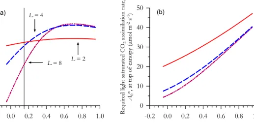
20

can thus estimate howA∗_CandA∗₀ should vary withkP for a givenLand this is shown in Fig. 1. Figure 1a shows that, as expected from theory (Field, 1983), the maximum A∗_C is indeed always observed when kI=kP=0.7. Also as expected, the higher the L, the greater the A∗_C at this optimum kP. But as kP declines (or increases) away from the optimum 0.7 value, the decline inACis much greater at higherL. So much so that

(7)

BGD

6, 4639–4692, 2009

J. Lloyd et al.

Title Page

Tables Figures

◭ ◮

Back Close

Full Screen / Esc

atkP=0.15 and with CCfixed (both being values which we consider typical for tropical forest of this region)ACcan actually decline with increasingL.

Figure 1b shows that changes inA∗₀that are required to satisfy Eq. (1) when CCis conserved. As kP increases then so does A∗0. This occurs because the necessary gradient within the plant canopy much be sharper whenkPis greater. Likewise, at any

5

givenkP then A∗0 is lower the greater the L. This is because the gradient in canopy photosynthetic capacity can effectively be spread over a greater depth ofL. We note already at this stage that Fig. 1b implies that there are certain combinations ofA∗₀,kP andCCwhich are not physiologically realistic. For example, most tropical tree species have maximum photosynthetic rates substantially less than 20 µmol m−2s−1 (Turner,

10

2001, p. 97). Thus an “optimum”kPmay not be possible – in the case of Fig. 1b unless CC were substantially lower (see Eq. 1). But this would, however, also mean thatAC was correspondingly reduced (again as shown in Sect. 2.3). This contradiction is the fundamental reason why “optima”kP as implied by Fig. 1a are not, in fact, optimal at all. That is to say, if one accepts that there is a fundamental limit to the maximum

15

photosynthetic rate possible for any given species, then the “optimum” kP requires a significantly lower canopy photosynthetic capacity werekPto be substantially lower.

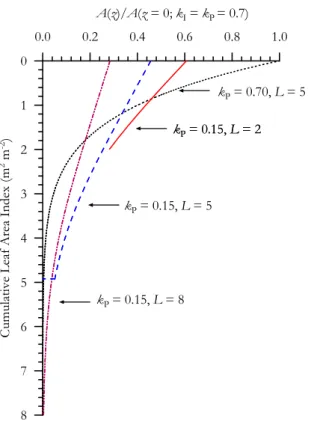
But why, despite higher canopy light interception, doesA∗_Cdecline with increasingL at lowkP? This also turns to be critical in Sect. 2.3 in determining what is the optimumL whenCCandA0are taken as fixed, and the answer can be seen from Fig. 2. Here, the

20

required gradients inAwithL are shown for various combinations ofkP andLwith all values standardised toA∗₀whenkI=kP=0.7. As would be expected from Fig. 1b, when kP<0.7 then A

∗

0 is also less than this “optimal case” and the greater isL; variation in photosynthetic the greater the reduction in A∗₀. The vertical variation photosynthetic losses or gains associated withkP 6= 0.7 can also easily be seen by comparing the

25

(8)

BGD

6, 4639–4692, 2009

J. Lloyd et al.

Title Page

Tables Figures

◭ ◮

Back Close

Full Screen / Esc

Atowards the top diminishes asL increases. As to why this occurs can be deduced from Fig. 1b. Because the high L/low kP combination necessitates a low maximum photosynthetic capacity at the top of the canopy, much of the relatively highQcannot be utilised. On the other hand, the extra photosynthetic capacity lower down is more or less wasted as CO₂assimilation rates at lowQare much less dependent onAmax(z).

5

It is for this reason that, other things being constant, the effective reduction inA∗_CaskP deviates from its “optimum value” increases asLincreases.

It is also worthwhile pointing out at this stage that the higher the value of A∗₀ the greater the relative “punishment” at any givenL. This is because any removal of pho-tosynthetic capacity away from the top of the canopy results in a proportionally greater

10

proportional loss inA∗_Cfor high capacity as opposed to low capacity trees (see Fig. 1b).

2.2 What constitutes the optimal combination ofLandkP?

As argued above, due to the highA∗₀required, what is often considered the “optimum” kPmay in fact not even be physiologically possible, especially when observation based values ofCC andL are employed. Indeed, it can even be argued that for such cases

15

the “optimality” question has previously been inappropriately posed. This is because, rather than asking what the optimum profile in photosynthetic capacity should for given values ofL andCC, one should rather be enquiring as to, given the considerable ge-netic and environmental limitations on A0 that undoubtedly occur (e.g. Wright et al., 2004; Fyllos et al., 2009). “What is the combination of L, CC and kP that serves to

20

maximise the net carbon gain of the canopy for any given value ofA0? To achieve this, we first write

NR=G_C∗ −RC−IC, (2)

whereNRis the net carbon gain to the canopy provided by the foliage on an annual ba-sis, after accounting for the investment of carbon as new leaves within the plant canopy,

25

(9)

BGD

6, 4639–4692, 2009

J. Lloyd et al.

Title Page

Tables Figures

◭ ◮

Back Close

Full Screen / Esc

the leaves in the absence of respiration in either the dark or the light. This is the same asA∗₀but, to increase confusion, is used for calculations on an annual timescale.

Noting also that elements such as nitrogen and phosphorus which are likely to be the key modulators of variations inAmax(z)tend to stay constant on a dry weight basis with depth within the canopy and with variations on an area being due to variations in leaf

5

mass per unit area (MA), see Discussion and references therein, then it then follows that we can simply expressICas

IC= I0e−kPz

z=L

z=0 =

I0(1−e

−k_PL

)

k_P , (3)

which ends up exhibiting the interesting property ofICnot varying withkPorLas long as CC and A0 are kept constant. To estimate I0 we assume an average leaf lifetime

10

(τ) of one year and taking typical values of M_A and carbon content for upper canopy leaves at Tapajos (88.5 g m−2and 491 mg g−1, respectively) obtain an estimate forI0of 4.5 mol C m−2for anA0of 12 µmol m−

2

s−1. Given that there is generally little correlation betweenA0and MAwhen the former is calculated on an area basis (Wright et al., 2004) we thus makeI0 independent ofA0and for simplicities sake (and noting that it has no

15

effect on the main conclusions of these simulations) we also makeτ independent of AmaxandI0.A

∗

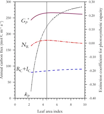
Cis calculated as in Eqs. (A4) and (A5) and integrated annually to obtain G_C∗, the model being driven by a dataset collected above the km87 tower at Tapajos (Goulden et al., 2004) consisting of about 3.8 years of net (incoming less reflected)Q averaged over hourly times steps and running from 1 July 2000–11 Mar 2004. Based

20

on data of Domingues et al. (2005) night time respiration (Rn) is simply calculated as 0.08CC but with, importantly, daytime respiration by the leaves within the canopy dependent upon the illumination received calculated through an analysis of the data of Atkin et al. (2000) according through Eqs. (A7) or (A8) and as shown in Fig. A1b and withRCvalues represent average annual sums.

25

Results from such a simulation are shown in Fig. 3 for our standard Tapajos condi-tions ofA0=12 µmol m

−2

s−1andCC=42 µmol m

−2

(10)

BGD

6, 4639–4692, 2009

J. Lloyd et al.

Title Page

Tables Figures

◭ ◮

Back Close

Full Screen / Esc

starting from a value of−0.35, with each increment sufficient to increase L by about 0.1−Lbeing calculated in each case through a rearrangement of Eq. (1).

As kP increases, the gradient away from the top of the canopy must by definition become sharper and, associated with this is an increase inL is required ; this being necessary to “hold”CC within a greater leaf area. Associated with this increase inkP

5

and L is first an increase in G_C∗ associated with an increase in light interception and withkPapproaching a similar value tokI. Nevertheless, asLincreases above a value of∼5.4, G_C∗ begins to decline. This is because of the aggravating e_ffects of higher L onkP/kIimbalances as demonstrated in the previous Section (Fig. 2) outweighing any advantage of increased light interception

10

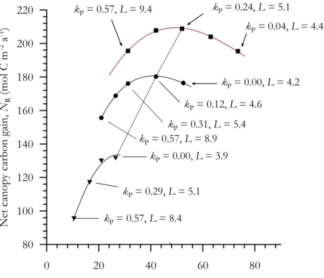
Although both IC and Rn do not change with the concurrent variations in kP and L, daytime respiration increases. This is because associated with higherL are more and more leaves at very low light levels where the inhibition of daytime respiration is considerably reduced (Fig. 1a). Thus, the net carbon gain of the canopy, IC peaks at intermediatekP and L, the optimum values for this simulation as being 0.123 and

15

4.5, respectively. These values compare surprisingly favourably with what is observed (kP∼0.15 as discussed above with L=5.1±0.5; Arag ˜ao et al., 2005), especially be-cause, as is discussed below, there are good reasons to think that both L and kP should infact be a little higher than the simple estimates predicted here. We also note that an estimate forG∗_Cof 262 mol C m−2a−1obtained from eddy covariance and other

20

measurements at the Tapajos tower (Hutyra et al., 2007) is in remarkably good agree-ment with our model based estimate ofG_C∗ of 265 mol C m−2a−1 at L=4.5. It is also worth noting here that althoughkP<0.0 (i.e. photosynthetic capacities increasing with canopy depth) is both mathematically and physiologically possible, if is also at odds with one central tenant of the approach here (viz thatA∗₀is a maximum physiologically

25

(11)

BGD

6, 4639–4692, 2009

J. Lloyd et al.

Title Page

Tables Figures

◭ ◮

Back Close

Full Screen / Esc

2.3 What constitutes the optimal combination ofA0andCC?

In Sect. 2.2, we took our best estimate of the integrated canopy photosynthetic ca-pacity for the Tapajos forest (A0=12 µmol m−

2

s−1andCC=42 µmol m− 2

s−1) and found, although e_ffects of variations in L and kP on G

∗

C, RC and NR were relatively modest, our model optimumNRhad associated with itGC∗,LandkPthat were surprisingly close

5

to those actually observed. But what happens with other combinations ofA0andCC? To the extent that foliar nutrient concentrations are related to variations in leaf photo-synthesis (Domingues et al., 2005; Mercado et al., 2009) the first should reflect some combination of genetic and environmental influences (Fyllas et al., 2009), whereas it might be reasonable to expect thatCC might be more strongly influenced by edaphic

10

conditions or climate than genotype, this being mediated through variations inLand/or kP.

To help answer this question, Fig. 4 therefore shows the results of simulations where we have kept the model driving Q as for Sect. 2.2, investigating now how NRvaries for three different photosynthetic capacities at the top of the canopy, viz

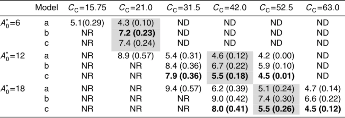
15

A∗₀=6 µmol m−2s−1, 12 µmol m−2s−1 and 18 µmol m−2s−1 and for a variety ofCC, the range of which examined depends on theA∗₀investigated (a highA∗₀/CCratio leads to unreasonably highL; conversely lowA∗₀/CC lead tokP<0.0). In all cases, the symbol plotted reflects that at the optimumNRas determined from simulations such as given on the graph in Fig. 3, with associatedkP andLshown for selected points.

20

This shows that, as might be anticipated, as CC increases from lower values, then so doesNR and that associated with this increasingNRare reductions in the optimal kP allowing the higher CC to be more evenly distributed over a smaller L: the lower Lreducing enhanced respiratory losses for high photosynthetic capacity leaves at the bottom of highCC canopies. Yet, there is also a clear maximum for eachA∗0, beyond

25

whichNRdeclines. This is because the enhancement inG

∗

(12)

BGD

6, 4639–4692, 2009

J. Lloyd et al.

Title Page

Tables Figures

◭ ◮

Back Close

Full Screen / Esc

the tree in terms of carbon losses.

Not surprisingly, theCCat which this point occurs increases withA

∗

0, with this being associated with a higher L and a higherkP. For A∗0=6 µmol m

−2

s−1 the optimal pre-diction is no gradient in photosynthetic capacity, with a tree with such a characteristic maximising its annual carbon gain by incorporating as much photosynthetic potential

5

into as small a leaf area as possible. AsA∗₀ increases the predicted “optimal” kP in-creases as a partitioning resources more in-line with the light distribution assumes relatively more importance, this also being associated with a higherL. But in no case is the predicted kP even close to that of the light extinction co-efficient (kI=0.7 in all simulations).

10

2.4 Evolutionarily stable versus instantaneous model solutions

From the above, estimates of within canopy gradients in photosynthetic capacity and leaf area index are intimately interrelated, and in indeed the earliest models of canopy structure and function (Monsi and Saeki, 1953) were based on the idea that the optimal leaf area index of a canopy would be that where the lowest leaves existed at the light

15

compensation point where daily leaf photosynthesis was just cancelled out by respi-ration (see also Hirose, 2005). Nevertheless, as pointed out by Anten (2002, 2005) such an calculation assumes that the optimum for an individual is not affected by the characteristics of its neighbours, being “simple optimization” in the sense of Parker and Maynard Smith (1990) This is to say, our above calculations so far have overlooked the

20

fact that by increasing it’sL above our estimated “optimum” value, a taller plant may also gain in it’s chances of survival and increase its rate long term growth by shading it’s neighbour(s). Looking at Fig. 4 then, one might conclude that for any given A∗₀, the “evolutionarily stable” optimal solution might, in fact, be somewhat to the left of the identified optimal value, with a slightly lowerNR and CC. Alternatively, whilst still

25

(13)

BGD

6, 4639–4692, 2009

J. Lloyd et al.

Title Page

Tables Figures

◭ ◮

Back Close

Full Screen / Esc

incurred in reducing the photosynthetic gain of one’s competitors was not balanced by the relative gain in increasing their losses. In a mathematical sense then, the optimal “evolutionarily stable”Lwould be one where

dNR dL ≥ −

dNC

dL , (4)

withNcrepresenting the net carbon gain of the competitors. Computing the right hand

5

term is di_fficult for such a heterogeneous systems as a tropical forest, but we have made a simple attempt of the likely effect assuming understory trees have a relatively low photosynthetic capacity ofA∗₀=5 µmol m−2s−1with aL=1.0 and withkP=0.15. Es-timates of the upper tree “evolutionarily stable”L so calculated from Eq. (4) (denoted L◦) are shown for selected combinations of A∗₀ and CC, together with L from the

“in-10

dividual optimization case” (Fig. 4) and a third estimate where the original Monsi and Saeki (1953) criterion is considered; viz. theLwhere and which the leaf at the bottom of the canopy has it’s photosynthetic carbon gain exactly balanced by it’s respiratory losses; in our case this “compensation point” representing the average photosynthesis and respiration rates over a 3 year period, denotedL∗.

15

This shows the “evolutionarily stable”L◦ can be as much as 3 m2m−2 greater than that calculated from Fig. 4 which is not that surprising given the only very slight re-ductions inNR that occur when L increases above its optimum value (Fig. 3). Note, however, thatL∗is often less thanL◦, and for the highestA∗₀/CCcombination, actually less thanLas inferred from Fig. 4. As is noted in the discussion, this is of considerable

20

consequence as although it is conceptually possible for a leaf at the bottom of a canopy to have a net negative carbon balance and still be a net benefit to the plant (it’s costs to the plant in terms of being a net sink for carbohydrates being more than offset by it’s gains to helping to shade a competitor), it seems this is not a physiologically vi-able possibility. This is because during leaf maturation, major physiological changes in

25

(14)

BGD

6, 4639–4692, 2009

J. Lloyd et al.

Title Page

Tables Figures

◭ ◮

Back Close

Full Screen / Esc

this effect occurs at much lower L(due to relatively higher respiratory costs) meaning that, despite the model as presented here initially predicting higherL with higher A∗₀, the ability for lowerA∗₀trees to sustain leaves at low light levels might mean they may be able actually maintain a higherL than their faster growing counterparts (Sterck et al., 2001; Kitajima et al., 2005).

5

3 Materials and methods

Of a total of a total of 1508 trees sampled in 65 permanent plots in Brazil, Bolivia, Colombia, Ecuador, Peru and Venezuela between January 2002 and April 2005 for foliar nutrients and other properties (Fyllos et al., 2009; Pati ˜no et al., 2009, 204 had also been sampled at three canopy heights for foliar nutrient composition, carbon and

10

nitrogen isotope ratios and leaf mass per unit area (M_A). Locations, vegetation and basic soil and climatological characteristics of the sample material plots are given in Pati ˜no et al. (2009) and Quesada et al. (2009).

3.1 Leaf sampling

Twelve to 40 trees per plot were chosen at random to collect upper canopy leaves

con-15

sidered to usually be exposed to the sun with the tree climber usually climbed three to eight trees in different points of the plot. From each climbed tree, braches of 1 to 2 m length from the exposed crown of two to four nearby trees were usually harvested. For randomly selected trees (generally three trees per plot) branches were additionally collected from the middle (sunny-shaded) and from the lower canopy (shaded) portion

20

of the canopy. Sampling was achieved by severing a branch (usually ca. 4 cm in di-ameter) from the tree, this being subsequently allowed to fall to ground. From each branch a sub-sample was made, generally distal to the area of twig used by Pati ˜no et al. (2008) for wood density analysis. One A4 sized plastic zip-bag of leaves of a range of possible different ages (but excluding obviously juvenile or senescencent leaves)

(15)

BGD

6, 4639–4692, 2009

J. Lloyd et al.

Title Page

Tables Figures

◭ ◮

Back Close

Full Screen / Esc

was then filled and sealed; kept as cool and shaded as possible and then transported to the laboratory or field station the same evening as the day of collection.

3.2 Tree and canopy height determinations

The heights of both the lowest branch and canopy of sample trees were determined using a clinometer (Model PM5/360 PC, Suunto, Turku, Finland) with “middle canopy”

5

leaves assumed to have been at the average crown height; calculated as the arithmetic mean of the upper and lower crown dimensions.

3.3 Leaf mass per unit area (MA)

Sub-samples of 10–20 leaves were taken for the leaves collected from each tree/measurement height combination and imaged using a locally purchased document

10

scanner attached to a Laptop or PC. The scanned images were then saved as image files analysed and with leaf area and other associated characteristics of each images subsequently analysed using Win Folia Basic 2001a (Regent Instruments, Quebec, QC, Canada). Scanning was usually done on the evening of collection, but when for lo-gistical reasons this was not possible, leaves were stored in tightly sealed plastic bags

15

for a maximum of two days to avoid desiccation and any associated reduction of the leaf area.

Once scanned, leaves were air dried in the field or when an oven was available they were dried at 70◦C for about 24 h or with a microwave oven in 5 min steps until death was considered to have been achieved. Once transported to the analysis laboratory

20

leaves were redried at 70◦C for about 24 h and their dry mass determined after being allowed to cool in a dessicator.

3.4 Sample preparation and analysis locations

Samples from Bolivia, Peru, Ecuador, Colombia and Venezuela were analysed in the Central Analytical and Stable Isotope Facilities at the Max-Planck Institute for

(16)

BGD

6, 4639–4692, 2009

J. Lloyd et al.

Title Page

Tables Figures

◭ ◮

Back Close

Full Screen / Esc

chemistry (MPI-BGC) in Jena, Germany. Samples from the Brazilian sites analysed for cations and phosphorus in at the Instituto Nacional de Pesquisas da Amaz ˆonia (INPA) in Manaus and for carbon and nitrogen in the laboratory of the Empresa Brasileira de Pesquisa Agropecu ´aria (EMBRAPA) in Manaus. In both laboratories leaf sample not used for MA determinations was dried as described above with a sub-sample of

5

about 20 g DW then taken, for which the main vein of all leaves was removed and the sub-sample subsequently ground. For Brazilian leaves, sub-samples of ground mate-rial were analysed for13C/12C ratios at the Centro de Energia Nuclear na Agricultura (CENA) in Piracicaba.

3.5 Carbon and nitrogen determinations

10

In both laboratories, analyses for C and N were carried out using 15–30 mg of finely ground plant material using a “Vario EL” elemental analyser (Elementar Analysensys-teme, Hanau, Germany). Inter-laboratory consistency was maintained via the regular use of the same CRM 101 spruce needle (Community Bureau of Reference, BCR, Brussels, Belgium) and SRM 1573a tomato leaf (National Institute of Standards of

15

Technology, Gaithersburg, MD, USA) standards in both laboratories. Within the Man-aus laboratory, laboratory consistency with Jena values was also checked from time to time by the comparison of ground rain forest tree foliar material of various C and N concentrations already previously analysed in Jena.

3.6 Cation and phosphorus determinations

20

In the Jena laboratory about 100 mg of sample material was first submitted to a microwave-assisted high pressure digestion (Multiwave, Anton Paar, Graz, Austria) after addition of 3 ml of 65% HNO3. Maximum reaction temperature was 230◦C with maximum pressures of 25–30 bar. To check for possible contamination of reagents and vessels, a blank was run with each series of standard reference materials or samples.

25

(17)

BGD

6, 4639–4692, 2009

J. Lloyd et al.

Title Page

Tables Figures

◭ ◮

Back Close

Full Screen / Esc

were transferred to 50 ml glass vessels which were filled to the mark with ultrapure water (Millipore, Eschborn, Germany) and analysed by ICP-OES (Model Optima 3300 DV, Perkin Elmer, Norwalk, CT, USA) with a 40 MHz, free-running RF-Generator and an array detector allowing for the simultaneous determination of the elements using wavelengths as given in Boumans (1987) and DIN EN ISO 11885 (1998).

5

In the Manaus laboratory, concentrations of P, K, Ca and Mg were determined af-ter digestion with a nitric/perchloric acid mixture is described in detail by Malavolta et al. (1989). Concentrations of K, Ca and Mg in the extracts were subsequently de-termined using a Atomic Absorption Spectrophotometer (Model 1100b, Perkin Elmer, Norwalk, CT, USA) as prescribed by Anderson and Ingram (1993). Phosphorus was

10

determined by colorimetry (Olsen and Sommers, 1982) using a UV visible spectropho-tometer (Model 1240, Shimadzu, Kyoto, Japan). As for the Jena laboratory to check possible contamination of reagents and vessels, a blank was run with each series of standard reference materials or samples. Inter-calibration between the two laborato-ries was achieved by the use of the same external and internal standards as for C and

15

N (Sect. 2.3).

3.7 Carbon isotope determinations

In the Jena laboratory,13C/12C isotopes were measured as described in Werner and Brand (2001). In short: within the same sequence of analyses, bulk tissue samples, laboratory reference materials (including quality control standards) and blanks were

20

combusted quantitatively using an NA 1110 elemental analyser equipped with an AS 128 autosampler (CE Instruments, Rodano, Italy) attached to a Delta-C isotope ratio mass spectrometer (Thermo-Finnigan MAT, Bremen, Germany) using a ConFlo III in-terface (Werner et al., 1999). In the CENA laboratory, Brazilian samples were analysed as described in Ometto et al. (2006). In brief, 1–2 mg of sample was combusted in an

25

(18)

BGD

6, 4639–4692, 2009

J. Lloyd et al.

Title Page

Tables Figures

◭ ◮

Back Close

Full Screen / Esc

Inter-calibration exercises between MPI-BGC and Jena using secondary standards and other plant material showed small but significant and systematic differences be-tween the two laboratories (r2=0.99). These have been corrected for in the results presented here in which results from the CENA laboratory have been accordingly ad-justed to provide full isotope scale equivalence with the Jena results.

5

4 Statistical analysis

4.1 Statistical analysis

As we were interested in vertical variations in foliar characteristics with individual trees and variations in these characteristics between individual trees as a function of canopy height (and not concerned with plot-to-plot variations – these are considered in Fyllas et

10

al., 2009) we used multilevel modelling techniques (Snijders and Bosker, 1999) treating both tree-to-tree variation (within a plot) and variations in overall mean values (between plots) as random (residual) effects, the Basin-wide average within tree and between tree gradients being determined according to

π_ℓtp =β0tp+β1hℓtp+β2hc+Rℓpt, (5)

15

whereπℓtpcan be taken to represent any physiological parameter of interest (measured on leaf “ℓ” within tree “t” located within plot “p”), β0tp is an intercept term which, as indicated by its nomenclature, was allowed to vary both between trees and between individual plots,β1is a coefficient that describes howπvaries with the height at which it was sampled (common to all leaves, trees and plots),β2is an additional co-efficient

20

describing how π_ℓtp varies with mean tree canopy height, hc, and Rℓtp is a residual term.

The tree and plot dependent intercept can be split into an average intercept and group dependent deviations. Firstly we write

β0tp=δ00p+U0tp, (6)

(19)

BGD

6, 4639–4692, 2009

J. Lloyd et al.

Title Page

Tables Figures

◭ ◮

Back Close

Full Screen / Esc

where δ00p is the average intercept for the trees sampled within each plot and U0tp is a random variable controlling for the e_ffects of variations between trees (i.e. with a unique value for each tree within each plot). Likewise, we also write

δ00p=γ000+V00p, (7)

whereγ000is the average intercept for the entire dataset andV00pis a random variable

5

controlling for the e_ffects variations between each plot (i.e. with a unique value for each plot). Using a general notation then, we can combine Eqs. (5–7) to yield

πltp=γ000+γ100hℓt+γ010hc+V00p+U0tp+Rℓtp, (8)

whereγ100describes how variations inπbetween leaves within a tree vary with canopy height (with the same value for all trees within all plots) and γ010 is a between-tree

10

regression coefficient that describes howπvaries with the overall (mean) canopy height (with the same value applying to all trees within all plots). For theV00p and U0tp, just as is the case for the Rℓtp, it is assumed they are drawn from normally distributed populations and the population variance of the lower level residuals (Rℓt) is likewise assumed to be constant across trees. Note that within each plot the mean value of

15

U0tp≡0 and likewise the mean value of V0tp≡0 for the dataset as a whole. As is the normal case in any regression model, within each tree the meanRℓtp≡0.

Equation (8) is a “three-level random intercept model” with leaves (level 1) nested within trees (level 2) which are themselves nested within plots (level 3). Associated with the three residual terms there is variability at all three levels and we denote the

20

associated variances as

var(R_ℓtp)=σ2, var(U0tp)=τ2,var(V00p)=φ2. (9)

The total variance between all leaves is σ2+τ2+φ2 and the population variance be-tween trees isτ2+φ2.

Equation (8) is flexible in that the within-tree regression coefficient is allowed to

dif-25

(20)

BGD

6, 4639–4692, 2009

J. Lloyd et al.

Title Page

Tables Figures

◭ ◮

Back Close

Full Screen / Esc

derivation in Chap. 4 of Snijders and Bosker (1999) considering the terms within a given tree, the terms can be reordered as

π_ℓtp =(γ000+γ010hc+U0t+V00p)+γ100hℓtp+Rℓtp. (10)

The random part between the parenthesis is the intercept for this tree and the re-gression coe_fficient for variation ofπ with height within trees isγ100. The systematic

5

(non-random) part is the within-tree regression line

π_ℓtp =(γ000+γ010hc)+γ100hℓtp. (11)

On the other hand, considering only the relationship between the average value ofπ within a canopy and the average canopy height,hC, then Eq. (10) becomes

π_.tp=γ000+γ010hc+γ100hc+V00p+U0tp, (12)

10

and the systematic part of the model can then be written as

π.tp=γ000+(γ010+γ100)hc. (13)

This shows that the between-tree regression coefficient is the random intercept model isγ010+γ100. Thus in the analysis which follows, when the relationship between any parameterπand height is di_fferent for between tree as opposed to within-tree variation

15

thenγ010 is significantly different from zero. Where this is not the case, any variation inπwith height is of a statistically similar magnitude irrespective of whether or not the source of variation is sampling at di_fferent heights within the one tree or comparing the average values for trees of different heights. All analyses were undertaken with the

MLwinN software package (Rabash et al., 2004). Heights were centred according to

20

(21)

BGD

6, 4639–4692, 2009

J. Lloyd et al.

Title Page

Tables Figures

◭ ◮

Back Close

Full Screen / Esc

5 Results

5.1 Sources of variation

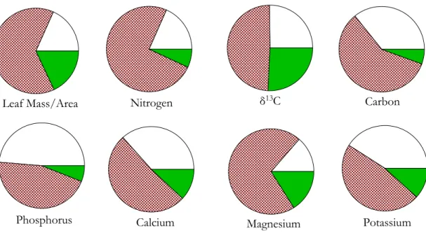
In order to examine the inherent sources of variability in the dataset, we first fitted a “null model” to untransformed data according to

π_ℓt =γ00+V00p+U0tp+Rℓtp. (14)

5

From this model and Eq. (9) the contribution of variations within and between trees and plots to the overall variance within the dataset can be simply apportioned and the results are shown in Fig. 5. This shows that, without exception, the variability observed in the eight π examined (MA and δ

13

C, with N, P, C, Ca, K and Mg on a dry weight basis) was greater between trees than the variance associated with the sampling of

10

the three different heights within trees. Moreover, the between-plot variance was also generally less than the within-plot (between tree) variance.

5.2 Vertical profiles

The underlying raw data giving rise to Table 2 and used in the subsequent multilevel analysis is shown for MA, [N]DW, [P]DW, [C]DW,δ

13

C and [Mg]DW in Fig. 6, with colours

15

coding for the different regions. This shows that, although there is considerable vari-ability in the data, certain patterns exist. For example, on average there is a trend for am increase in MAwithhand the opposite is the case forδ

13

C. On the other had, gen-erally speaking concentrations in [N]DW and [P]DW are quite consistent within a given tree, although there are of course exceptions, especially at higher concentrations.

Fo-20

(22)

BGD

6, 4639–4692, 2009

J. Lloyd et al.

Title Page

Tables Figures

◭ ◮

Back Close

Full Screen / Esc

From Fig. 6 there is considerable heteroscedastity in the data with the variance of the dependent variables tending to increasing with their absolute value but independent of the value of the independent (height variable). This was the case for allπ except maybe C andδ13C. Moreover, an examination of residual variances showed marked departures from normality, even when plot-to-plot di_fferences in overall mean values

5

were taken into account. We therefore transformed all data (taking the absolute value ofδ13C) prior to analysis, fitting the equation

log_e(πℓtp)=γ00+γ10hℓt+γ01hc+V00p+U0tp+Rℓtp. (15)

Results are listed in Table 2, for which the null hypothesis that a certain regression parameter (γh) is zero (i.e. H0: γh=0) can be tested according to (”) (two tailed t

-10

test T(γh)=γˆh/[S.E.( ˆγh)], the so called Wald test. This indicates (as shown in bold font) that within tree canopy gradients were significantly di_fferent to zero only for M_A, [C]DW, δ

13

C and [Mg]DW. From Eq. (13), the parameter γ010 reflects the difference between the within-tree and between-tree slopes but a separate Wald test can be used to determine if the overall co-efficient for the between tree coefficient (γ₁₀₀+γ₀₁₀) is

15

significantly different from zero (Snijders and Bosker, 1999). From such an analysis we can conclude

1. The between tree coefficient for MA is not significantly different to the within tree co-efficient and both show M_A are significantly different to zero. Both increase with increasing height.

20

2. There is no detectable within-tree gradient for nitrogen, phosphorus of calcium when expressed on a dry-weight basis. Nor is overall, there any significant overall tendency for mean canopy nitrogen or phosphorus concentrations to increase with mean canopy height.

3. Foliar|δ13C|decreases with height irrespective of whether the source of variation

25

(23)

BGD

6, 4639–4692, 2009

J. Lloyd et al.

Title Page

Tables Figures

◭ ◮

Back Close

Full Screen / Esc

higher leaves within the same tree. The gradients with height are similar for both sources of variation and are both significantly di_fferent from zero.

4. There is a significant tendency for [C]DW to increase with height within an individ-ual tree, and also for taller trees to have a higher foliar C content.

5. Although there is a significant tendency for [Mg]_DW to decrease with increasing

5

height within a given tree, the opposite pattern is observed for the variation be-tween trees. Taller trees tend to have significantly higher [Mg]DW than shorter ones. Potassium also shows a significant tendency to decrease with increasing height within a given tree, but, contrary to magnesium with this effect perhaps being amplified, rather than reversed, when tree-to-tree variation is considered.

10

Figure 7 shows the fitted slopes and the data, in all cases normalised to the fitted value for each tree at the average sampling height of 19.8 m. Here a comparison of the plots for within-tree and between-tree variation show the generally similar increases for MA with height and in decreasesδ13C and [C]DW with height, irrespective of the source of variation. On the other hand, the much steeper gradient for [K]_DW when

between-15

tree variations are considered is also apparent as the strong contrast in directions for [Mg]DW. Taller trees tend to have higher [Mg]DW, but within individual trees [Mg]DW declines with height. Though not significant, the trends for slightly decreased [N] and [P] with height in individual tree canopies can also clearly be seen.

5.3 Area based profiles

20

Vertical variations [N] and/or [P] within canopies can be expected to substantially influ-ence tropical forest canopy photosynthetic rates which are normally expressed per unit leaf area (Carswell et al., 2000; Domingues et al., 2005; Mercado et al., 2009), and it is also thus of interest to examine vertical gradients within and between trees also expressing nutrients on a leaf area basis (Table 3) – this simply being calculated as

25

(24)

BGD

6, 4639–4692, 2009

J. Lloyd et al.

Title Page

Tables Figures

◭ ◮

Back Close

Full Screen / Esc

similar and significant positive gradients to exist for both nitrogen [N]A) and phospho-rus [P]_A) and, although not significantly di_fferent, the between tree gradients are in both cases about 50% steeper than the within-tree gradients. The negative gradient in CA as on a DW basis is maintained, as is the positive gradient for KA, though in the case of K_Athe between-tree gradient is no longer statistically stronger than observed within

5

individual trees. The pattern for magnesium is also very different on leaf-area versus dry-weight basis. The negative DW gradient (lower values higher up in the canopy) is counterbalanced by the positive gradient in M_A meaning that within individual tree canopies no gradient in Mg exists. On the other hand, the positive between-tree gradi-ent in magnesium is amplified when expressed on an area basis.

10

Leaf area based gradients for nitrogen and phosphorus are shown in Fig. 8, again with each tree having its value normalised to the fitted value at the average sampling height of 19.8 m This illustrates the similar overall patterns observed for NA and PA, a result that is not surprising as a comparison of Fig. 8 with Fig. 7 in conjunction with Tables 2 and 3 shows that almost all the variation observed in NA and PA; both within

15

and between trees is due to the increase inMA with height with [N]DW and [P]DW on a dry weight basis varying little with height and with [N]_DW perhaps even decreasing slightly. From a consideration of measured average leaf area indices of the canopies examined (ca. 5.4; Pati ˜no et al., unpublished) in conjunction with the average canopy depth as measured by the differences in height between the top of the tallest and the

20

bottom of the lowest trees, we estimate that the average combined within/between tree gradient for the forests examined would relate to an extinction coefficient when expressed as a function of cumulative leaf area index (as per the accompanying model simulations in this paper,kP) of only around 0.10. Nevertheless, such a calculation is necessarily rough as it involves assumptions about the relative contribution of

within-25

(25)

BGD

6, 4639–4692, 2009

J. Lloyd et al.

Title Page

Tables Figures

◭ ◮

Back Close

Full Screen / Esc

5.4 Do tree-to-tree variations in within-canopy gradients exist?

The analysis so far has assumed that the within-tree gradients are the same for all sites and trees, but that different sites and the trees within them trees may assume different overall nutrient concentrations (a “random intercept model”) But, especially in light of the model results of Sect. 2, it is also of interest to determine if the gradients really

5

do differ between trees, and if so, in a systematic way. Given the “noise” apparent in Fig. 6, this is obviously not an easy question to answer, but it can be tested by takingβ1tp=γ100hℓtp+U1tphℓtp (see Eq. 5), this then adding an additional random term to Eq. (8) viz,

πℓtp =γ000+γ100hℓtp+γ010hc+V00p+U0tp+U1tphℓtp+Rℓtp. (16)

10

The additional term allows different trees to have different within-canopy gradients – a so called “random slope model” (Snijders and Bosker, 1999) with a χ2 test then employable to see if the model fit has been improved. And indeed, when this was attempted, it was found that significant tree-to-tree variation in within canopy gradi-ents was observed for MA, |δ

13

C| and PA (but not for [N]A). Moreover, as is shown

15

in Fig. 9 these variations in slopes (or “extinction coefficients”) were not random, but inter-related and correlated with the mean MA,|δ

13

C| and PA of the trees concerned. In particular, all three were well correlated with mean canopy PA, this being the aver-age of all three measurements taken on each tree, denotedh[P]_Ai, with the very similar patterns for the gradients in M_Aand P_Awithh[N]_Aisuggesting that most of the between

20

tree variability in within canopy gradients in PAwas due to variations in MArather than [P]DW. The strong decline in |δ

13

(26)

BGD

6, 4639–4692, 2009

J. Lloyd et al.

Title Page

Tables Figures

◭ ◮

Back Close

Full Screen / Esc

6 Discussion

That plants can acclimate to different light levels at chloroplast, leaf and canopy has long been appreciated (Monsi and Saeki, 1953; Boardman, 1977; Bj ¨orkman, 1981) and a key focus of recent years has been understanding the way plants that allocate their resources throughout their canopies, with one key focus being photosynthetic carbon

5

gain (Niinemets, 2007). It was Field (1983) who first proposed that plant photosynthetic carbon gain would be optimized if key physiological resources required for photosyn-thesis (in his case nitrogen) were allocated in direct proportion to the par received. This idea of “optimization” is conceptually attractive with this assumption even being incorporated into some canopy gas exchange models (Lloyd et al., 1995; Sands, 1995;

10

Sellers et al., 1996). But it is also now clear that although the decline in photosynthet-ically important elements such as nitrogen and phosphorus within plant canopies can be considerable and even impressive, this is never to the same degree that it matches the decline in the light environment (De Jong and Doyle, 1985; Carswell et al., 1980; Meir et al., 2002; Anten 2005; Wright et al., 2006).

15

As to why this should be so has proved somewhat of an enigma, it being generally accepted that natural selection should have resulted in plants optimising their resource strategies and various hypotheses have been proposed to account for this apparent “non-optimality”. These include the fact that plants do not grow as isolated individuals with bur rather in competition with others (Anten, 2005), that it might be related to

20

direct versus diffuse radiative transfer (Alton and North, 2007) or not all nitrogen being related to photosynthesis (Hikosaka, 2005); that there may be optimisation of N to light gradients within leaves as well as canopies (Terashima et al., 2005); that the required high very nitrogen concentrations at the top of the canopy may place leaves at strong risk of herbivory (Stockhoff, 1994); that there may be considerable costs of

25

(27)

BGD

6, 4639–4692, 2009

J. Lloyd et al.

Title Page

Tables Figures

◭ ◮

Back Close

Full Screen / Esc

generally driven by gradients in MA rather dry-weight variations (Reich et al., 1998; Evans and Poorter, 2001) that there may be a practical lower limit to the minimum M_A and hence NA that any species can achieve (Meir et al., 2002).

Though with some affinity with the latter the suggestion, the answer we present to this long standing apparent discrepancy di_ffers to other suggestions made to date.

5

That is to say: The optimality question has actually been incorrectly posed. And we suggest from our simulations and results presented here that once correctly posed, it turns out gradients of photosynthetic resources within plant canopies are, in fact, close to optimal.

For example, in some cases it has simply been assumed that the problem is simply

10

one of allocating resources for a canopy of a given leaf area index and photosynthetic capacity (as observed). But when this is done (e.g. dePury and Farquhar, 1995) what emerges are unrealistically high nutrient concentrations being required at the top of the canopy, inconsistent with the physiological tradeo_ffs that clearly exist in terms of leaf structure and function (Wright et al., 2004). This is similar to the point of Meir et

15

al. (2002) already mentioned above, that there is probably also a realistic lower limit to the M_A and nutrient content that any species can attain.

Although flexibility no doubt exists it also is now well established that different species have different characteristic maximum values of MA, [N] and [P] (Fyllas et al., 2009), this being closely linked to other aspects of their physiological strategy including leaf

lifes-20

pans (Wright et al., 2004) and hydraulic characteristics (Santiago et al., 2004; Pati ˜no et al., 2009). Thus the optimisation question should also be viewed within the constraints of these known physiological boundary conditions such as the maximum (species de-pendent) photosynthetic potential of the leaves at the top of the canopy, and, in some cases, the practical minimum value achievable at the bottom of the canopy, this

per-25

haps being structural (as suggested by Meir et al., 2002), or alternatively being a con-sequence of the need for all leaves to maintain a positive carbon balance once mature (Turgeon, 2006), as discussed in Sect. 2.4.

(28)

BGD

6, 4639–4692, 2009

J. Lloyd et al.

Title Page

Tables Figures

◭ ◮

Back Close

Full Screen / Esc

the individual lines shown in Fig. 4. A plant with an “optimal” distribution of it’s photo-synthetic resources (highkP) unavoidably has less photosynthetic resources than one that does not (low kP). Thus, it is actually to a plants advantage to have a shallow gradient in photosynthetic resources as this allows it to have a greater overall photo-synthetic capacity (Cc) and hence a higher net rate of carbon gain, NR. As discussed

5

in Sect. 2.4, it turns out there are several complexities which end up influencing the minimumkP and maximum NR which should occur, but nevertheless, the theory and model as presented here does lead to the (intuitive) prediction that plant with a low overall photosynthetic capacities should have shallower gradients in their photosyn-thetic resources than those with higher photosynphotosyn-thetic capacities. This can be inferred,

10

for example, if we accept that phosphorus has a role in the photosynthetic process for tropical tress (Raaimakers et al., 1995; Lloyd et al., 2001) from the relationship between h[P]Ai and the gradients shown in Fig. 9. It is also consistent with greater di_fferences between sun and shade leaves in M_A and many other leaf characteristics (including PA) for dependent species (as opposed to obligate-gap species or

gap-15

independent species) observed by Popma et al. (1992) for a tropical forest in Mexico, with the gap-dependent species also having higher N_A and P_A a than the other two species groups.

As is evidenced from Fig. 8 this tree-to-tree variation in the gradients in MA and P_A are also accompanied by correlated variations inδ13C, this suggesting that that for

20

such trees compensating gradients in stomatal conductances do not necessarily occur. Gradients in height were also observed in plant carbon contents, both within and between trees. Small within canopy gradients in [C]DW have been reported before by Poorter et al. (2006) who accounted for lower construction costs of low irradiance leaves in terms of lower levels of soluble phenolics. Studying upper-canopy leaves

25

from across the Amazon Basin, Fyllas et al. (2009) also observed significant variations in foliar carbon content, relating this to variations in M_A and the extent of investment in constitutive defences.

(29)

BGD

6, 4639–4692, 2009

J. Lloyd et al.

Title Page

Tables Figures

◭ ◮

Back Close

Full Screen / Esc

trees is the tendency for leaves higher up rain forest canopies to have greater levels of carbon based defence compounds (Lowman and Box, 1983; Downum et al., 2001; Dominy et al., 2003), this perhaps being associated with higher abundances of herbi-vores such as insects and other arthropods also occurring there (Sutton, 1989; Kato et al., 1995; Koike et al., 1998; Basset et al., 2001).

5

The decrease in [Mg]_DW with height within individual trees (Table 2, Fig. 7) seems similar to that reported by Grubb and Edwards (1982) comparing saplings and mature trees within a New Guinea montane rain forest. They attributed this to the central role of Mg within the chlorophyll (Chl) complex (Shaul, 2002) with increased [Chl]_DW for shaded leaves being a well documented phenomenon (Boardman, 1977; Bj ¨orkman,

10

1981) – as generally seems to be also the case for tropical forest trees (Rozendaal et al., 2006). The intra-tree Mg gradient was not, however, significant when expressed on a leaf area basis, despite both [N]_Aand [P]_Adeclining with increasing canopy depth. Particularly for N this is consistent with the idea that in shaded conditions a large por-tion of N is invested in chlorophyll for light capture, leading to a high Chl:N ratios. On

15

the other hand, for light exposed leaves a large proportion of N is invested in Ru-bisco with commensurate low Chl: N ratios (Poorter et al., 2000; Evans and Poorter, 2001). On the other hand, it was also found that [Mg]Aincreased with height along with

[N]_Aand [P]_Awhen inter-tree differences in tree height were the source of vertical vari-ation (Table 3), even though when comparing different rain forest trees [Chl]_A seems

20

to be independent of light environment or tree height (Rijkers et al., 2000). Probably then, this increase in [Mg]_A with tree height relates to its other physiological functions, for example in the process of thylakoid acidification (Pottosin and Sch ¨onkmecht, 1996), as an activator of several photosynthetic enzymes including Rubisco (Gardemann et al., 1986; Portis, 1992) and as a ATP-cofactor required for phloem loading of sugars

25

(Shaul, 1992). All these physiological functions would be expected to need to be pro-ceeding at higher rates in taller trees with higher [N]A and [P]A. This is because such

(30)

BGD

6, 4639–4692, 2009

J. Lloyd et al.

Title Page

Tables Figures

◭ ◮

Back Close

Full Screen / Esc

interception compared to trees occurring lower down the canopy stratum.

Appendix A

Gradients of photosynthetic capacity in plant canopies

As shown by Field (1983) the photosynthetic rate of a canopy of a given leaf area index

5

(L) andQ0 is the incident photon irradiance at the top of the canopy photosynthetic capacity should be maximised if throughout that canopy nitrogen, or any other factor considered to be limiting for photosynthesis was distributed in direct proportion to the photon irradiance (Q). A similar situation exists for the photosynthetic machinery of leaves (Farquhar, 1989). Although conceptually attractive in terms of an optimisation

10

of valuable resources and as a tool for modelling studies (Lloyd et al., 1995; Haxeltine and Prentice, 1996; Sellers et al., 1996), numerous field observations have shown this not, infact be the case. Gradients of nitrogen in particular are generally less than those predicted by the Field (1983) model (Meir et al., 2002; Wright et al., 2006). Here we show why this should be the case.

15

We first start with a general equation describing the photosynthesis the light depen-dence of photosynthesis, the rectangular hyperbola, viz:

A_z = Amax(z)φQz Amax(z)+φQz

−R_z, (A1)

whereAz represents the net CO2 assimilation rate of a leaf at some point, z, within the canopy,Amax(z)is the maximum net CO2assimilation rate of the leaf in question (at

20

light saturation),φis the quantum yield,Q_z is the photon irradiance at the leaf surface and Rz is the rate of respiration by the leaf. Equation (A1) is of a slightly different

form to that of a rectangular hyperbola usually presented (Causton and Dale, 1990), allowing a constant φ (independent of Amax(z)). From both empirical and functional points of view better equations exist, for example the monomolecular (Causton and