Autoregressive modelling of species richness in the Brazilian Cerrado

Vieira, CM.

_{*, Blamires, D}

_{, Diniz-Filho, JAF.}

_{*, Bini, LM.}

_{and Rangel, TFLVB.}

a_{Departamento de Biologia, Unidade Universitária de Ciências Exatas e Tecnológicas – UnUCET,} Universidade Estadual de Goiás – UEG

b_{Programa de Pós-Graduação em Ciências Ambientais, Universidade Estadual de Goiás – UEG} c_{Unidade Universitária de Quirinópolis, Universidade Estadual de Goiás – UEG,} Av. Brasil, Qd. 03, Lt. 01, s/n., Conjunto Hélio Leão, CEP 75860-000, Quirinópolis, GO, Brasil d_{Departamento de Biologia Geral, Instituto de Ciências Biológicas – ICB, Universidade Federal de Goiás – UFG,}

CP 131, CEP 74001-970, Goiânia, GO, Brasil

e_{Departamento de Ecologia e Biologia Evolutiva, University of Connecticut Storrs, CT 06269-3043, USA} *e-mail: diniz@icb.ufg.br, cleiber.marques@ueg.br

Received March 24, 2006 – Accepted May 30, 2007 – Distributed May 31, 2008 (With 4 figures)

Abstract

Spatial autocorrelation is the lack of independence between pairs of observations at given distances within a geo-graphical space, a phenomenon commonly found in ecological data. Taking into account spatial autocorrelation when evaluating problems in geographical ecology, including gradients in species richness, is important to describe both the spatial structure in data and to correct the bias in Type I errors of standard statistical analyses. However, to effectively solve these problems it is necessary to establish the best way to incorporate the spatial structure to be used in the models. In this paper, we applied autoregressive models based on different types of connections and distances between 181 cells covering the Cerrado region of Central Brazil to study the spatial variation in mammal and bird species rich-ness across the biome. Spatial structure was stronger for birds than for mammals, with R2 _{values ranging from 0.77 to}

0.94 for mammals and from 0.77 to 0.97 for birds, for models based on different definitions of spatial structures. According to the Akaike Information Criterion (AIC), the best autoregressive model was obtained by using the rook connection. In general, these results furnish guidelines for future modelling of species richness patterns in relation to environmental predictors and other variables expressing human occupation in the biome.

Keywords: spatial autoregression, species richness, Cerrado, birds, mammals.

Modelagem por auto-regressão da riqueza de espécies no Cerrado Brasileiro

Resumo

Autocorrelação espacial é definida como a falta de independência entre pares de observações a uma dada distância geo-gráfica e é um fenômeno muito freqüente em dados ecológicos. É importante levar em consideração os efeitos de autocor-relação espacial em ecologia geográfica, tanto para realizar uma descrição mais detalhada dos dados quanto para corrigir estimativas enviesadas do erro Tipo I das análises estatísticas convencionais. Entretanto, para resolver efetivamente esses problemas, é preciso avaliar a melhor forma de incorporar estruturas espaciais nos modelos. Neste estudo, modelos au-toregressivos, baseados em diferentes tipos de conexões e distâncias entre 181 células de uma rede cobrindo a região do Cerrado brasileiro, foram ajustados para avaliar a variação espacial de riqueza de mamíferos e aves dentro do bioma. A es-trutura espacial foi ligeiramente mais forte para aves do que para mamíferos, com valores de R2 _{variando entre 0,77 e 0,94}

para mamíferos e 0,77 e 0,97 para aves, em modelos baseados em diferentes formas de conexão espacial. Segundo o Critério de Informação Akaike (AIC), o modelo autoregressivo melhor ajustado foi obtido através da conexão “em torre”. Em geral, esses resultados fornecem diretrizes para futuras modelagens dos padrões de riqueza de espécies que estão asso-ciados a preditores ambientais e/ou a variáveis que expressam a ocupação humana no Cerrado.

Palavras-chave: autoregressão espacial, riqueza de espécies, Cerrado, aves, mamíferos.

1. Introduction

Autocorrelation is the lack of independence be-tween pairs of observations at given distances in time or space and is commonly found in ecological dataset (Legendre, 1993; Legendre and Legendre, 1998; Fortin and Dale, 2005). Many recent papers have discussed the

respectively. Data from the literature (Marinho-Filho et al., 2002; Eisenberg and Redford, 1999; Emons, 1990; Embrapa, 2002; Fonseca et al., 1996) and specifically the following biodiversity websites were used to map the species: The Revista Brasileira de Zoologia (RBZ) site, SpeciesLink site, The Animal Diversity Web site (The University of Michigan Museum of Zoology) and the Site of the Global Biodiversity Information Facility Data Portal (GBIF) (a detailed species list and references are available from the authors upon request). A binary ma-trix was constructed by recording the geographic ranges of which species overlapped each cell, and species rich-ness was calculated by summing the species present in the cells. Geographical coordinates of cell centroids (latitude and longitude) were also obtained for further spatial analyses.

2.2. Spatial description

Spatial autocorrelation measures the similarity be-tween samples for a given variable as a function of spatial distance (see Legendre and Legendre, 1998). For quan-titative variables, such as species richness, the Moran’s I coefficient is the most commonly used coefficient in uni-variate autocorrelation analyses and is given by:

I = n S

y - y y - y w_{i j ij}

j i

2 i y - yi

(1)

where n is the number of cells, y_i and yy are the values_j of the species richness in cells i and j, y is the average of y and w_ij is an element of the matrix W. In this matrix, papers show that autocorrelation analyses can be useful

to provide a more detailed description of spatial structure in species richness data and to allow a better understand-ing of ecological processes drivunderstand-ing richness (Legendre, 1993; Diniz-Filho et al., 2003). At the same time, it is now widely recognized that testing statistical hypotheses using standard methods (e.g., ANOVA, correlation and regression) in the presence of spatial autocorrelation will cause downward bias in the standard errors and, consequently, Type I error rates may be strongly inflated (Haining, 1990, 2003; Cressie, 1993; Legendre, 1993; Fortin and Dale, 2005).

Description of spatial patterns in data using cor-relograms and variograms is now straightforward (see Legendre and Legendre, 1998; Fortin and Dale, 2005). On the other hand, incorporating the autocorrelation structure into modelling, in a regression framework, may be a more complicated task. Autocorrelation analysis must be based on the spatial relationship between spatial units, but this must be established by taking into account the relationship between the processes underlying diver-sity and the geographic distances or connectivity among the spatial units analysed. For example, in a stream net-work, it is important to consider the links between units along the river flows and to take into account ecological barriers (Ganio et al., 2005). Formally, these alternative propositions must be codified into a weighting matrix

W. However, for broad-scale patterns in species

rich-ness in terrestrial systems, it is difficult to establish these connections assuming spatial dynamics of ecological or biogeographical processes. Empirical evaluation of alter-native spatial modelling strategies may be an initial solu-tion, especially considering that models can be sensitive to misspecifications in the W matrix (Cressie, 1993).

In this paper, we evaluated the spatial patterns of mammal and bird species richness in the Brazilian Cerrado. Our goal is to discuss how changes in the defi-nition of the spatial relationship among spatial units (i.e., grid cells) affect the statistical performance of the autore-gressive models describing species richness. This may provide a basis for further analyses investigating the rela-tionship between the environmental predictors and rich-ness and consequently allow a better evaluation of the processes driving the spatial patterns in species richness.

2. Material and Methods

2.1. Data

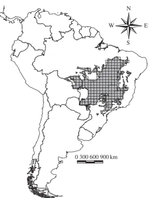
The extents of occurrence of the 138 non-volant mam-mals species (Marinho-Filho et al., 2002) and 751 birds species (Ridgely and Tudor, 1989, 1994; del Hoyo et al., 1992; 1994; 1996; 1997; 1999; 2001; 2002; Junniper and Parr, 1998; Silva, 1995) found in the Brazilian Cerrado were mapped with a spatial resolution of 1º grid cell, with a total of 181 cells covering the Cerrado Biome (Figure 1). The gathered information on the mammals included 8 or-ders: Didelphimorphia, Xenarthra, Primates, Carnivora, Rodentia, Perissodactyla, Artiodactyla and Lagomorpha,

0 300 600 900 km N

S

W E

Figure 1.Distribution of the 181 cells that were used to

We also used seven different criteria to create binary (0 or 1) matrices W, indicating whether pairs of locali-ties are connected or not. We used the Delaunay trian-gulation, Gabriel, the Minimum Spanning Tree and the Relative Neighbour networks, and established rook and queen connections among the cell centroids (Figure 2; see also Legendre and Legendre, 1998; Fortin and Dale, 2005, for details). These connections are built using dif-ferent criteria to establish the links among the cells. In short, according to the Delaunay Triangulation Criterion, for a triplet of points (i.e., cell centroids) to be connected, a circle that circumscribes them (i.e. the circle passing through the three points) must include no other points, whereas in Gabriel connections, two points are con-nected if the circle in which the diameter is the distance between the points includes no other points. According to the Relative Neighborhood Criterion, two points are connected if, and only if, there is no other points lying on the intersection between the two circles centered in the two points, whereas in the Minimum Spanning Tree all points are inter connected so that the length of this connection is the minimum possible. Rook and Queen connections are designed to match ‘chess’ movements (see Figure 2).

The autoregressive models based on these 15 different matrices W (6 binary connectives and dis-tance-based using 9 values of ) were compared using different approaches, for mammal and bird richness. The R2 _{values of the autoregressive model indicate the}

abil-ity of each model to explain spatial structure in richness, whereas an autocorrelation analysis base on Moran’s I in the term indicates the effectiveness in taking auto-correlation structure into account. Akaike information criterion (AIC) was also used to select the best model, within an information theory framework (see Burham and Anderson, 2002, for details). For each model, AIC corrected for small samples was computed as:

AIC = n log( 2_{) + 2K (n/n – K – 1) (4)}

where n is the number of cells, K is the number of pa-rameters in the model and 2 _{is the variance of the}

re-siduals of each regression model. The variance of the residuals was used here as a proxy for the likelihood of the model given the data (Haining, 2003), whereas the term (n/n – K – 1) is the small sample correction term and tends to one as n increases. We compared the AIC

values of each model using AIC, which is the differ-ence between AIC of each model and the minimum AIC found. A value higher than 10 indicates that a model has a poor fit relative to the best model, whereas a value less than 3 indicates that a model is equivalent to the best model (with the lowest AIC); model. The AIC values were also used to compute Akaike’s weighting of each model (w), which provides evidence that the model is actually the best explanatory model. The values of w are usually standardized by their sum among all models evaluated, so they are dependent on the set of models used and are given by:

w_ij= 1 if the pair i,j of cells is within a given distance class interval (indicating cells that are “connected” in this class), and w_ij = 0 otherwise. S indicates the number of entries (connections) in the W matrix. The value ex-pected under the null hypothesis of absence of spatial autocorrelation is –1/(n–1). Detailed descriptions of the computations of the standard error of this coefficient are given in Legendre and Legendre (1998).

Moran’s I usually varies between –1.0 and 1.0, for maximum negative and positive autocorrelation, respec-tively. Non-zero values of Moran’s I indicate that rich-ness values in cells connected at a given geographic distance are more similar (positive autocorrelation) or less similar (negative autocorrelation) than expected for randomly associated pairs of cells. The geographic tances among cell centroids can be partitioned into dis-crete classes, creating then successive W matrices and

allowing computation of different Moran’s I values for the same variable. This allows one to evaluate the pat-terns of autocorrelation as a function of spatial distance, in a graph called spatial correlogram, which furnishes a spatial description of the species richness. The number and definition of distance classes to be used in the cor-relograms are arbitrary, but a general methodological criterion is to try to maximise the similarity in the S val-ues (number of connections) for the different Moran’s I coefficients, so that they are more comparable. In this paper, correlograms were based on 15 distance classes (see Figure 4).

2.3. Spatial modelling

Spatial autocorrelation in mammal and bird rich-ness (y) was modelled by an autoregressive model of the form:

y = Wy + ฀

whereW is the row-standardized weighting matrix (not decomposed as in the correlogram), is the autoregres-sive parameter and is the error vector. This model must be fitted by maximum likelihood procedures (Haining, 1990; 2003; Cressie, 2003). Squared correlation between y and the estimated value ( Wy) furnishes the pseudo-R2

of the model, expressing the proportion of variance in Y that is explained by an autoregressive process.

The autoregressive model above was fitted using various W matrices, derived from alternative ways to

establish relationships between the spatial units (cells in the Cerrado grid). First, geographic distances among the cell centroids was used, and values in the matrix W were obtained using inverse-powered functions, given by:

w_ij = 1 / D_ij (3)

–6 –7 –8 –9 –10 –11 –12 –13 –14 –15 –16 –17 –18 –19 –20 –21 –22 –23 Latitude

–60 –58 –56 –54 –52 –50 –48 –46 –44 –42 Longitude

D < 150 km –6_–7

–8 –9 –10 –11 –12 –13 –14 –15 –16 –17 –18 –19 –20 –21 –22 –23 Latitude

–60 –58 –56 –54 –52 –50 –48 –46 –44 –42 Longitude

D < 200 km

–6 –7 –8 –9 –10 –11 –12 –13 –14 –15 –16 –17 –18 –19 –20 –21 –22 –23 Latitude

–60 –58 –56 –54 –52 –50 –48 –46 –44 –42 Longitude Delaunay triangulation –6 –7 –8 –9 –10 –11 –12 –13 –14 –15 –16 –17 –18 –19 –20 –21 –22 –23 Latitude

–60 –58 –56 –54 –52 –50 –48 –46 –44 –42 Longitude Gabriel criterion –6 –7 –8 –9 –10 –11 –12 –13 –14 –15 –16 –17 –18 –19 –20 –21 –22 –23 Latitude

–60 –58 –56 –54 –52 –50 –48 –46 –44 –42 Longitude Relative neighbour –6 –7 –8 –9 –10 –11 –12 –13 –14 –15 –16 –17 –18 –19 –20 –21 –22 –23 Latitude

–60 –58 –56 –54 –52 –50 –48 –46 –44 –42 Longitude

Minimum spanning tree

w = exp(–1/2 AIC)/ _i[exp(–1/2 AIC_i)] (5)

All spatial analyses were performed in SAM (Spatial Analysis in Macroecology; Rangel et al., 2006), which is

a software freely available at www.ecoevol.ufg.br/sam.

3. Results

Both mammal and bird species richness show a clear spatial pattern in the Brazilian Cerrado, with higher richness concentrated in the south-eastern region of the biome, decreasing toward the north (Figure 3). High

count. In principle, models based on binary connections are better than models based on the inverse of geographic distances.

The AIC analysis allowed a more effective compari-son among these alternative models (Table 1). In both mammals and birds, there is no model with AIC small-er than 3, indicating that, in principle, thsmall-ere is a unique solution for modelling richness. The best models were obtained using the rook connection (Figure 2), and the standardized Akaike weights suggest a chance higher than 99.9% that these are the best models among those tested. They yield R2 _{values of 0.938 and 0.972 for}

mam-mals and birds, respectively. Coherent with patterns re-vealed in the spatial correlograms, birds display stronger spatial structure than mammals, with higher fit of autore-gressive models.

However, it is interesting to note that Moran’s I in the best model residuals for mammals displays a relatively high negative autocorrelation value –0.193, so a slight over-correction of the spatial structure probably occurred in this case (see Griffith, 2002). For both mammals and birds, the second best models were based on the Gabriel network (Figure 2), although AIC is slightly larger than 10, indicating a low chance that this is the best model and, for mammals, the residual autocorrelation is still relatively high (–0.143).

4. Discussion

Different forms of autoregressive models have been recently applied in geographical ecology (Lichstein et al., 2002; Kelt and Tognelli, 2004; Fortin and Dale, 2005). These models have been mainly used as a way to take the spatial structure into account in data and, at the same time, to evaluate how different environmental predictors are related to spatial variations in species rich-ness. However, in most of these papers, researchers as-sume a given form of matrix W and do not explore alter-native scenarios for the relationship among spatial units and the weighting of autoregressive model.

Our results show that the autoregressive model, used here only to analyse spatial structure in richness, is rather sensitive to variations in the definition of W and,

con-richness values also appear in the western region of the biome, but this patch is clearer for mammals. Indeed, spatial correlogram confirm this strong spatial structure, with Moran’s I coefficients large in the first distance class (0-245 km) and decreasing monotonically with the increasing of geographic distances (Figure 4).

Autoregressive modelling based on the different W

matrices (Table 1) reveals a large variation in model fit, both for mammals and birds. As expected, connections based on the minimum spanning tree were not adequate and showed a very poor fit, and will be not considered further. The R2 _{values ranged from 0.77 to 0.94 for}

mam-mals and from 0.77 to 0.97 for birds. Relatively high values of Moran’s I (i.e., I 0.1) remain in the residu-als of a few models. In these cases, modelling was not effective in taking the autocorrelation structure into

ac-0 3ac-0ac-0 6ac-0ac-0 9ac-0ac-0 km Birds

Species Richness

N

S

W E

516-572 573-629 630-686 687-742 743-799 800-856

0 300600 900km Mammals

Species Richness

N

S

W E

49-53 54-58 59-62 63-67 68-71 72-76

Figure 3. Mammals and birds species richness variation across the Brazilian Cerrado.

Distance (km)

Moran's I

–1.0 –0.8 –0.6 –0.4 –0.2 0.0 0.2 0.4 0.6 0.8 1.0

0 500 1000 1500 2000 2500 Mammals Birds

it is important to consider that a negative autocorrela-tion in the residuals remains, so a more careful evalua-tion should be performed. In practice, the consequence is that the effect of environmental predictors would be underestimated due to the overestimation of the spatial component in species richness. Of course, more complex models could be tested using alternative scenarios, for example taking into account the different biogeographi-cal or ecologibiogeographi-cal boundaries based on vegetation types or historical barriers, but this is beyond the scope of this paper.

We provide here guidelines for a more effective modelling of the richness patterns of mammals and birds sequently, using these models to relate richness to

en-vironmental predictors requires more effort around the definition of W.

We recognize that it is difficult to find theoretical ar-guments to support the use of a given W matrix to

ate richness patterns at broad scales, so empirical evalu-ations, as performed here, are important. In our analysis of the mammals and birds in the Cerrado, AIC-based model selection was which effective in establishing a single model as the best one, based on a rook connec-tion among cells. A model based on Gabriel connecconnec-tions followed this, according to AIC. For mammals, although AIC selected the rook connection as the best model,

Table 1. Results of the autoregressive models including the following statistics: Coefficient of determination (R2_), autoregres-sive parameter ( ), standard error (SE), number of parameters (K), Akaike Information Criterion (AIC), residuals’ autocor-relation (as estimated by the Moran’s I coefficient), difference between AIC of each model and the minimum AIC found ( (AIC)), Akaike’s weighting of each model (w_i) and standardized w_i (w_i/w_t).

or connection

R2 _{SE K AIC Moran’s} I

(AIC) w_i w_i/w_t

Mammals

Distance 1.0 0.773 0.870 0.051 2 1257.27 0.194 235.4 0.000 0.0000 Distance 1.5 0.810 0.880 0.036 3 1227.46 0.137 205.6 0.000 0.0000 Distance 2.0 0.840 0.901 0.025 3 1195.61 0.079 173.8 0.000 0.0000 Distance 2.5 0.862 0.906 0.019 3 1169.63 0.023 147.8 0.000 0.0000 Distance 3.0 0.874 0.904 0.016 3 1153.14 –0.016 131.3 0.000 0.0000 Distance 3.5 0.871 0.898 0.014 3 1144.59 –0.036 122.7 0.000 0.0000 Distance 4.0 0.882 0.893 0.014 3 1140.46 –0.043 118.6 0.000 0.0000 Distance 4.5 0.883 0.888 0.013 3 1138.74 –0.044 116.9 0.000 0.0000 Distance 5.0 0.884 0.884 0.013 3 1138.10 –0.041 116.3 0.000 0.0000 Connection Delaunay 0.914 0.899 0.007 2 1081.06 –0.087 59.2 0.000 0.0000 Connection Gabriel 0.934 0.902 0.004 2 1032.86 –0.143 11.0 0.004 0.0041 Connection MST 0.403 0.288 0.356 2 1432.55 0.753 410.7 0.000 0.0000 Connection RNJ 0.916 0.814 0.007 2 1076.56 0.103 54.7 0.000 0.0000 Connection Rook 0.938 0.921 0.004 2 1021.85 –0.193 0.0 1.000 0.9960 Connection Queen 0.891 0.893 0.012 2 1124.18 –0.048 102.3 0.000 0.0000 Birds

ronmental predictors and other variables expressing hu-man occupation in the biome.

Acknowledgements –– Financial support for this study came from a PRONEX program of CNPq and SECTEC-GO (proc. 23234156). Work by JAFDF and LMB was also partially supported by other CNPq projects (grants number 300762/94-1 and 300367/96-1; respectively). CAPES and FUNAPE-UFG have also continuously supported our research program in macroecology and biodiversity.

References

ALLEN, AP., BROWN, JH. and GILLOOLY, JF., 2002. Global biodiversity, biochemical kinetics, and the energetic-equivalence rule,Science, vol. 297, no. 5586, p. 1545-1548.

ARAÚJO, MB., 2003. The coincidence of people and biodiversity in Europe, Global Ecol. Biogeogr., vol. 12, no. 1, p. 5-12.

BADGLEY, C. and FOX, DL., 2000. Ecological biogeography of North American mammals: species density and ecological structure in relation to environmental gradients, J. Biogeography, vol. 27, no. 6, p. 1437-1467.

BALMFORD, A., MOORE, JL., BROOKS, T., BURGESS, N., HANSEN, LA., WILLIAM, P., and RAHBEK, C., 2001. Conservation conflicts across Africa, Science, vol. 291, no. 5513, p. 2616-2619.

BURHAM, KP. and ANDERSON, DR., 2002. Model selection and multimodel inference. A practical information-Theoretical Approach. New York: Springer-Verlag.

CRESSIE, NAC., 1993. Statistics for spatial data. New York: John-Wiley and Sons, Inc.

CURRIE, DJ., MITTELBACH, GG., CORNELL, HV., FIELD, R., GUEGAN, JF., HAWKINS, BA., KAUFMAN, DM., KERR, JT., OBERDORFF, T., O’BRIEN, E. and TURNER, JRG., 2004. Predictions and tests of climate-based hypotheses of broad-scale variation in taxonomic richness. Ecol. Lett., vol. 7, no. 12, p. 1121-1134.

Del HOYO, J., ELLIOT, A. and SARGATAL, J. (eds.), 1992, Handbook of the birds of the world: ostrichs to ducks. vol. 01. Barcelona: Lynx Edicions.

-,Handbook of the birds of the world: new world vultures to guineafowl. vol. 02, Barcelona: Lynx Edicions

-, 1996, Handbook of the birds of the world: hoatzin to auks. vol. 03, Barcelona: Lynx Edicions.

-, 1997, Handbook of the birds of the world: sandgrouse to cuckoos. vol. 04, Barcelona: Lynx Edicions.

-, 1999, Handbook of the birds of the world: barn-owls to hummingbirds. vol. 05, Barcelona: Lynx Edicions.

-, 2001, Handbook of the birds of the world: mousebirds to hornbills. vol. 06, Barcelona: Lynx Edicions.

-, 2002, Handbook of the birds of the world: mousebirds to woodpeckers. vol. 07, Barcelona: Lynx Edicions.

DINIZ-FILHO, JAF., BINI, LM., PINTO, MP., RANGEL, TFLVB., CARVALHO, P., and BASTOS, RP., 2006. Anuran species richness, complementarity and conservation conflicts in Brazilian, Cerrado, Acta Oecol., vol. 29, no. 1, p. 9-15.

in the Brazilian Cerrado. In some sense, it matches the theoretical evaluation by Griffith (1996), who gave some advice on choosing between alternative W matrices. For predictive purposes, using any of the models discussed here is better than assuming that no spatial autocorre-lation exists, especially considering the relative high R2 _{values of all autoregressive models. This indicates}

that ignoring spatial components using ordinary regres-sion models (OLS) probably will furnish biased results. Another important guideline is the preference of using low order (= short distance) expressions of spatial struc-ture, in which close localities are more heavily weighted, when compared to distant ones. Indeed, our results show that the AIC values based on connections are usually higher than those obtained with the inverse distances functions. Also, there is a perfect decrease in AIC values when increasing the values. However, Griffith (1996) indicated that over-specification of the connections in the model (in this case, generating high negative autocorre-lation in the residuals of the model) is worse than under-specification. Thus, although rook connections were se-lected by AIC as the best model, followed by Gabriel connections, future modelling must be aware of inflated negative spatial structures in residuals and, eventually, further models may be tested if more complex autore-gressive models are to be obtained (i.e., by adding envi-ronmental predictors – see below).

envi-LEGENDRE, P. and envi-LEGENDRE, L., 1998. Numerical ecology. Amsterdam: Elsevier.

LEGENDRE, P., 1993. Spatial autocorrelation: trouble or new paradigm?Ecology, vol. 74, no. 6, p. 1659-1673.

LENNON, JJ., 2000. Red-shifts and red herrings in geographical ecology, Ecography, vol. 23, no. 1, p. 101-113.

LICHSTEIN, JW., SIMONS, TR., SHRINER, SA. and FRANZREB, KE., 2002. Spatial autocorrelation and autoregressive models in ecology, Ecol. Monog., vol. 72, no. 3, p. 445-463.

MARINHO-FILHO, J., RODRIGUES, FHG., and JUAREZ, KM., 2002. The Cerrado mammals: diversity, ecology, and natural history. In OLIVEIRA, PS. and MARQUIS, RJ (eds.), The Cerrados of Brazil. New York: Columbia University Press. p. 266-284.

RAHBEK, C. and GRAVES, GR., 2001, Multiscale assessment of patterns of avian species richness, P. Natl. Acad. Sci.-Biol., vol. 98, no. 8, p. 4534-4539.

RIDGELY, R. and TUDOR, G., 1989. The birds of South America (vol I- the oscine passerines). Austin: University of Texas Press.

-, 1994, The birds of South America (vol. II- the suboscine passerines). Austin: University of Texas Press.

SILVA, JMC., 1995. Birds of the cerrado region, South America, Steenstrupia, vol. 21, no. 1, p. 69-92.

TOGNELLI, MF. and KELT, DA., 2004. Analysis of determinants of mammalian species richness in South America using spatial autoregressive models, Ecography, vol. 27, no. 4, p. 427-436.

DINIZ-FILHO, JAF., BASTOS, RP., RANGEL, TFLVB., BINI, LM., CARVALHO, P. and SILVA, RJ., 2005. Macroecological correlates and spatial patterns of anuran description dates in the Brazilian Cerrado, Global Ecol. Biogeogr., vol. 14, no. 5, p. 469-477.

DINIZ-FILHO, JAF., BINI, LM. and HAWKINS, BA., 2003. Spatial autocorrelation and red herrings in geographical ecology, Global Ecol. Biogeogr., vol. 12, no. 1, p. 53-64.

FORTIN, MJ. and DALE, M., 2005. Spatial analysis: a guide for ecologists. Cambridge: Cambridge University Press. GANIO, LM., TORGERSEN, CE. and GRESSWELL, RE., 2005. A geostatistical approach for describing patterns in stream networks, Front. Ecol. Environ., vol. 3, no. 3, p. 138-144. HAINING, R., 2003. Spatial data analysis. Theory and Practice. Cambridge: Cambridge University Press.

HAINING, R., 1990. Spatial data analysis in the social and environmental sciences. Cambridge: Cambridge University Press.

HAWKINS, BA., PORTER, EE. and DINIZ-FILHO, JAF., 2003. Productivity and history as predictors of the latitudinal diversity gradient of terrestrial birds, Ecology, vol. 31, no. 6, p. 1608-1623.