On the use of pseudo-forces to consider initial conditions in 3D time- and frequency-domain acoustic analysis

On the use of pseudo-forces to consider initial conditions

in 3D time- and frequency-domain acoustic analysis

C.J. Martins

, J.A.M. Carrer

, W.J. Mansur

, F.C. Arau´jo

a_{Department of Civil Production Engineering, CEFET, 30510-000 Belo Horizonte, MG, Brazil} b_{PPGMNE/Federal University of Parana´, CP 19011, 81531-990 Curitiba, PR, Brazil} c_{Department of Civil Engineering, COPPE/UFRJ, CP 68506, CEP 21945-970 Rio de Janeiro, RJ, Brazil}

d_{Department of Civil Engineering, UFOP, 35400-000 Ouro Preto, MG, Brazil}

Received 17 February 2004; received in revised form 13 September 2005; accepted 14 September 2005

Abstract

This work is mainly concerned with a general strategy, based on well known concepts of classical mechanics, for taking into account initial conditions in frequency-domain (FD) and time-domain (TD) analyses. A general approach, extended here to three-dimensional applications, is presented. Special problems associated with analyses through Discrete-Fourier-Transform (DFT) algorithms, as those occurring in consequence of a non-correct choice of extended period or those connected with aliasing phenomenon, are also discussed. Furthermore, an alternative starting procedure for time-marching schemes (in TD analyses) is proposed. At the end of the paper, to val-idate the proposed techniques and to demonstrate their generality, two- and three-dimensional problems with non-homogeneous initial conditions are solved through frequency- and time-domain approaches by employing the Finite Element Method (FEM). Numerical results are compared with existing analytical solutions.

2005 Elsevier B.V. All rights reserved.

Keywords: Finite element method; 3D wave equation; Frequency- and time-domain analyses; Initial conditions

1. Introduction

According to the nature of the dynamic problem to be solved, the numerical solution can be sought either in the time-domain or in transformed time-domains. Although time-time-domain formulations can be efficiently adopted for solving a great range of problems, in some cases the analysis via transformed domains (e.g. frequency, Laplace or wavelet domains)

is the only feasible alternative [25,7,11]. Particular attention will be devoted here to the frequency-domain approach

[25,7,22] that has been extensively used in analyses in which the physical parameters, such as the damping in soil– structure interaction problems, are frequency-dependent. Practical problems in which the analyses of dynamic systems

are carried out in the frequency domain are presented by Wolf[28], related to soil–structure interaction problems, Clough

and Penzien [7], related to structural systems, Hall [12] and Kinsler [15], related to FEM modeling of acoustic

prob-lems, and Beskos [3], Dominguez [8], Brebbia [4] and Banerjee [1], related to engineering problems modeled with the

BEM.

A great deal of attention has been devoted to turn the frequency-domain approach more efficient. One of the deficiencies

of the Fourier analysis, as described by Thomson[25], Clough and Penzien[7], Paz[22], Oppenheim and Schafer[21], is

0045-7825/$ - see front matter 2005 Elsevier B.V. All rights reserved. doi:10.1016/j.cma.2005.09.007

* _{Corresponding author.}

E-mail address:webe@coc.ufrj.br(W.J. Mansur).

concerned with the periodic nature of the Fourier transform and, consequently, with the difficulty of considering initial

conditions. In spite of the importance of this topic, to the best of the authorsÕ knowledge, only a few works concerning

this matter have been presented until now. Venancio-Filho and Claret[27]presented the concept of the Implicit Fourier

Transform (ImFT), extended later to non-linear problems by Mansur et al. [17]. Veletsos and Ventura [26] employed

the Green_Õs function and its time derivative in modal coordinate analyses, and in Soares and Mansur [24] the inverse

discrete Fourier transform of the steady state Green_Õs function is carried out to obtain the corresponding

time-domain GreenÕs function for SDOF mechanical systems. The techniques described above, in spite of being efficient and

of taking into account initial conditions, are applied to problems described by modal coordinates (i.e., SDOF mechanical systems).

The present work describes a quite general method to take into account initial conditions. The proposed method, which

is based on the concepts of pseudo-forces, see Refs.[9,18], and generalized functions[6], will be applied to the solution of

three- and two-dimensional scalar problems, in the time- and frequency-domain, modeled with finite elements. Initially, the time-dependent and frequency-dependent partial differential equations governing wave propagation problems are pre-sented. Then the corresponding algebraic systems of equations are shown. A discussion concerning DFT-based analysis, which emphasizes the special role played by the extended period of analysis and by the aliasing phenomenon in the acqui-sition of the numerical response, is also presented.

The steps adopted to take into account the initial conditions, related to the potential and its time derivative, in

fre-quency-domain analyses are presented. In addition, the method previously presented by Mansur et al.[18]for 2D problems

is extended to 3D frequency- and time-domain applications.

Finally, aiming at validating the described algorithms, the results from the analyses of two- and three-dimensional prob-lems with non-homogeneous initial conditions, in time- and frequency-domain, are presented and compared with analytical results.

2. The wave propagation problem

The scalar wave equation is usually associated with the description of vibrational phenomena, such as the vibration of strings and membranes, and the propagation of acoustic waves and electric signals along wires. In its general form, the

associated initial boundary value problem is given by (see[19,20])

qo

2 uðx;tÞ

o_t2 r ðEruðx;tÞÞ ¼fðx;tÞ in X; ð1Þ

with the boundary conditions

uðx;tÞ ¼uðx;tÞ on Cu;

pðx;tÞ ¼ouðx;tÞ

o_nðxÞ ¼pðx;tÞ onCp

ð2Þ

and the initial conditions

uðx;0Þ ¼u0ðxÞ inX; ð3Þ

_

uðx;0Þ ¼u_0ðxÞ inX. ð4Þ

In the above equationsu(x,t) denotes the scalar solution,f(x,t) the domain source function, andqandEthe medium

den-sity and YoungÕs modulus respectively.

The solution of Eq.(1), under harmonic excitations, can be assumed to behave harmonically with angular frequencyx,

if a long enough time has elapsed after the occurrence of initial disturbances. In this way, the problem is said to be sta-tionary. The physical variables of the acoustic problem can be represented as follows:

uðx;tÞ ¼Uðx;xÞeixt_{; fðx;tÞ ¼Fðx;xÞe}ixt_{; pðx;tÞ ¼Pðx;xÞe}ixt_{; ð5Þ}

whereU(x,x),F(x,x) andP(x,x) are complex functions. After substituting expressions(5)into Eq.(1)and eliminating

the exponential function eixt_{, the resulting Helmholtz}

Õs equation can be written as

qx2Uðx;xÞ þ r ðErUðx;xÞÞ ¼ Fðx;xÞ in X. ð6Þ

The boundary conditions to Eq.(6) are given by

Uðx;xÞ ¼Uðx;xÞ on Cu;

Pðx;xÞ ¼Pðx;xÞ on Cp.

2.1. Spatial discretization

The Finite Element Method (FEM) was adopted as a numerical tool for the solution of the scalar wave Eq.(1) (see

[29,2,14]). The resulting system of linear algebraic equations can be written as

MU€þCU_ þKU¼R. ð8Þ

MatricesM,CandKrepresent, respectively, mass, damping and stiffness global matrices.

For harmonic problems, one hasU(t) =Uxeixt_and

R(t) =Rxeixt₍

UxandRxrepresent the nodal potential and nodal

flux amplitudes respectively); thus the corresponding system of equations reads

ðx2MþixCþKÞUx¼Rx. ð9Þ

2.2. Damping

A usual way to add damping to the system is by expressing its viscous damping matrix,C, proportional to the mass and

stiffness matrices (RayleighÕs damping model). By assuming stiffness-proportional damping, sayc=a1E(cdenotes the

vis-cous damping coefficient associated with the continuum model), its implementation in the FD formulations can be directly

carried out by substituting YoungÕs modulus,E, by the following complex one:

Ed_{¼Eð1þixa1Þ; witha}

1¼

c

E; hence E

d_{¼Eþixc. ð10Þ}

As seen above, the viscous damping assumes frequency-dependent energy dissipation. This assumption is sometimes

non-realistic (see [25,7]). Indeed, experimental observations show that the dissipated energy is frequency-independent

for a great deal of materials employed in engineering at a wide frequency range. In this case, the following frequency-inde-pendent damping model (hysteretic damping) should be used instead

Ed_{¼Eð1þigÞ; ð11Þ}

wheregis the hysteretic damping coefficient.

2.3. Nyquist frequency

In order to obtain the solution of transient dynamic problems by a frequency-domain formulation, the Fourier trans-form is applied to the time-dependent excitation. Subsequently, after the response spectrum is determined (i.e. solving Eq.

(9)), the synthesis of the frequency-dependent spectrum is carried out via inversion. The number of time sampling points

must be chosen so that the highest excitation frequency in the Fourier spectrum be higher than the highest frequency (that

matters) of the discretized mechanical system at hand (see[21,23,5]); this excitation frequency is the so-called Nyquist

fre-quency, defined as

xNyq ¼

Np

T ; ð12Þ

whereNis the number of sampling points andT is the total time of analysis. The consequence of the violation of this

condition is an incorrect superposition of effects, leading to a distortion of the inverse Fourier transform (aliasing phenomenon).

2.4. Extended period

The Fourier transform is based on the assumption that the external excitation and the system response are periodic in time. Hence, to attain a correct response to a non-periodic loading, it is necessary to extend the time of analysis up to a time

Tp,the extended period, so that atTpthe system is at rest. IfTpis large enough, the causality condition is obeyed, i.e.,

per-turbations acting before the initial time will not influence the response in the interval of interest. Since the prediction of the

extended period,Tp, is inadvisable in practice, it must be estimated. In previous works, e.g. Refs.[17,24], the extended

per-iod has been estimated as a time interval longer than any time required to damp down the first mode contribution

(mea-sured, for instance, in terms of displacement amplitudes) toh percent of its initial contribution. Thus, by following this

approach, the extended period can be established according to the relation

TpP

lnð100=hÞ

n1x1

wheren1is the damping ratio associated with the first mode andx1is the fundamental frequency of the system. Usually,

1% is adopted forh.

3. Contribution of initial conditions to transient problems

The correct specification of the initial conditions plays an important role in the description of time-dependent problems. The method developed here introduces initial conditions via pseudo-forces in 3D frequency- and time-domain modeling. The time-domain strategy is new, and so is the 3D frequency-domain approach, which allows for non-trivial initial

con-ditions[25,7,22].

3.1. Initial displacement

First, only the initial displacement field is imposed to the system. The initial velocity field is assumed to be null and no external forces are applied. The basic step consists in substituting the initial displacement field by static pseudo-forces

which generate the given initial displacement field. An equivalent pseudo-force vector, FU, is obtained according

to FU=K1U0, U0being the known nodal initial displacement vector. Note that FUis an external static force vector,

applied to the system previously to the initial time of the analysis, which generates the initial fieldU0. The system motion

starts by the application of a nodal equivalent force vectorFUatt= 0, which generates a displacement fieldDUt,

com-puted by

MDU€tþCDU_tþKDUt¼ FUHðtÞ ¼ KU0HðtÞ; ð14Þ

whereH(t) is the Heaviside function (or unit-step function), see[20]. One can assume that the total displacement field,Ut,

for the present case, is constituted of two parts: one due to the action of the field force represented byFUH(t) and the other

due to the initial displacement field. Thus

Ut ¼DUtþU0. ð15Þ

In frequency-domain analyses, the equivalent pseudo-force vector,FU, is incorporated to the system by following a

sim-ilar procedure. The final equation is

ðx2MþixCþKÞDUx¼ FUHx¼ KU0Hx; ð16Þ

wherexis the Fourier transform parameter andHxis the Fourier transform of the Heaviside function. Analogously to

expression(15), the total complex displacement field can be computed as a sum of two parts, as follows:

Ux¼DUxþdðxÞU0. ð17Þ

It is important to note that if the DFT (or FFT) algorithm is employed, the Heaviside function,H(t), must be replaced by

the productH(t)[1H(tT/2)]. In this case, the extended period must be considered twice that of the initial guess

(ob-tained for instance from expression(13)).

3.2. Initial velocity

The contribution due to an initial velocity field can be obtained from the following concepts of classical mechanics

(under the assumption of constant mass, [10,16]):

Momentum(Q): The momentum is a conservative quantity. It is defined as follows:

Q¼mv. ð18Þ

Impulse(I): The impulse is defined as the time integral of the force, given by

I¼ Z Dt

0

Fdt¼m Z Dt

0

dv

dt dt. ð19Þ

The impulse–momentum relation states that the impulseIacting on the mass will result in a change in the momentum and,

consequently, in its velocity. If the mass is initially at rest, one can write

I¼mv0. ð20Þ

Then, the contribution of an initial velocity field,V0¼U_ð0Þ, can be taken into account by the pseudo-force FVdefined

below[20,6]

whered(t) is the Dirac delta function. Thus, the displacementUtdue to the presence of an initial velocity field can be com-puted from

MU€tþCU_tþKUt¼FV¼MU_ðtÞdðtÞ. ð22Þ

In the frequency domain, the Fourier transform of the Dirac delta function is equal to the unity, hence the corresponding transformed equation of motion is given by

ðx2MþixCþKÞUx¼MV0. ð23Þ

It must be observed that the Fourier transform ofFV, which is equal toMV0, must be corrected when DFT algorithms

are employed. As shown by Clough and Penzien[7]: DFTðMV0dðtÞÞ ¼_N1_DtMV0, whereNDt=T.

3.3. General case

When the structure is subjected to the action of external forcesRtunder non-homogeneous initial conditionsU0andV0,

the system of equations is written as (in the time-domain)

MDU€tþCDU_tþKDUt¼RtKU0HðtÞ þMU_ðtÞdðtÞ; ð24Þ

where

Ut¼DUtþU0. ð25Þ

Alternatively to classical starting procedures for time-marching schemes (see[2,14]), the time-step procedure can be

ini-tialized using the new initial conditions in the deformed state, given by

DU0¼DU_0¼0. ð26Þ

In this case, the loading vector of the dynamic equilibrium equation, Eq.(24), is given by

RtKU0þ

MV0

Dt at t¼0 and R

t_KU

0 fort>0. ð27Þ

In frequency-domain analyses, the complex response in the transformed domain is obtained from

ðx2MþixCþKÞDUx_¼

RxKU0HxþMV0; ð28Þ

where the complex displacement field is given by

Ux¼DUxþdðxÞU0. ð29Þ

4. Applications

4.1. Rod under a Heaviside type forcing function and initial conditions prescribed all over the domain

In this example, a prismatic rod fixed at one end and free at the other is analyzed (see[31]). For the discretization, 4000

lagrangean linear hexahedral elements where employed, which gives 4961 degrees of freedom, seeFig. 1. The rod length is

L= 1.2 m and its cross-section area is A= 0.3 m·_{0.3 m. The longitudinal wave propagation velocity and density are}

respectivelyc= 1000 m/s and q= 0.01 kg/m3. The rod is subjected to the initial conditions

U0¼ p₀L

E z

L; 06z6L;

V0¼ p₀c

E ; c¼ ffiffiffiffi E q s

06z6L;

8 > > > <

> > > :

withp₀¼100 N=m2_{. ð30Þ}

In expressions(30),Eis the Young_Õs modulus. Additionally, a Heaviside type-forcing functionp0H(t) is applied at the free

end of the rod. This problem was analyzed through the time- and frequency-domain formulations. For the FD analysis, the

extended periodTp= 0.196 s and 4096 sampling points were adopted. It must be pointed out that the extended period,Tp,

calculated by considering modal damping ration1= 0.0125 and modal frequencyx1ffi1309 rad/s, corresponds toh= 4%

(i.e., reduction to 4% of the first mode contribution). In the TD analysis, the implicit damped HHT scheme[13]was used

with:Dt= 0.00005 s,a¼ 1

9;c¼12a;b¼

ð1aÞ2

4 , and total time of analysisTa= 0.0096 s (192 time steps). In the FD

anal-ysis, a hysteretic damping coefficientg= 2n1= 0.025 was adopted. The proportionality factor used for taking into account

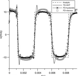
2 and 3present the response at the free end of the rod in terms of displacement and velocity, respectively. A good agree-ment between numerical and analytical responses is observed.

4.2. Rod under a Heaviside type forcing function and initial conditions prescribed in part of the domain

In this example, the following initial conditions are imposed to the rod analyzed in the previous example:

U0¼

1 4

p₀L

E z

3L

4

₄

L;

3L

4 6z6L;

V0¼ p0c

E ; c¼ ffiffiffiffi E q s

; 3L

4 6z6L;

V0¼U0¼0; 06z<

3L 4 ; 8 > > > > > > > > < > > > > > > > > :

withp₀¼100 N=m2_{. ð31Þ}

Again, the HHT time-marching scheme was adopted for the time-domain analysis with the same parametersa,b, andc, the

same time step and total time of analysis as in the previous example. The values of the hysteretic and viscous damping

coefficients are the same as well. Once more, the results agree quite well with each other.Figs. 4 and 5present, respectively,

the displacement and velocity at the free end of the rod.

0 0.002 0.004 0.006 0.008

t(s) 0 0.005 0.01 0.015 0.02 0.025 u(m) Analytic TD-HHT FD-hysteretic FD-viscous

Fig. 2. Displacement time-history at the free end of the rod under Heaviside-type forcing function and initial conditions prescribed all over the domain. x

y z

L

p0

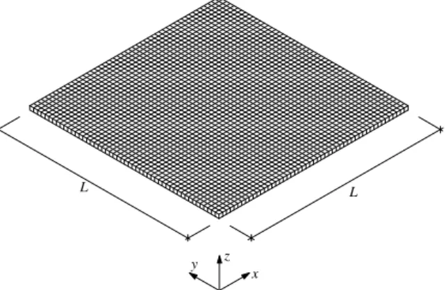
4.3. Square membrane under prescribed initial velocity: 3D and 2D analyses

This example consists of a square membrane of side L= 50 cm, subjected to zero initial displacements in its entire

domain and the initial velocity field described below (seeFig. 6):

V0¼

100c

EA ; if L

46x6

3L

4

\ L

46y6

3L

4

\ ½06z6h;

0; in the remainder of the domain.

8 <

:

ð32Þ

The following parameters were adopted:c= 1000 cm/s andq= 0.01 kg/cm3_{. In the 2D analysis, 20,000 isoparametric}

linear triangular elements were adopted. In the 3D analysis 2500 isoparametric parabolic continuum elements were

employed (seeFig. 7). In the frequency-domain analyses, 4096 sampling points and an extended periodTp= 2.5 s,

esti-mated to reduce the contribution of the first mode (x1ffi89 rad/s,n1= 0.05) toh= 1.49·103% of its initial contribution,

were adopted. In the TD analysis, the implicit HHT method was applied to march on time.Dt= 0.0001 s and 1250

time-steps were employed. A hysteretic damping coefficient g= 2n1= 0.10 was adopted. The corresponding

stiffness-propor-tional viscous-damping factor (adjusted by the first mode, and used for both HHT and viscous-damping frequency-domain

analyses) is a1= 1.13·103. Note that a TD analysis without damping via HHT scheme with parameters a= 0.00,

b= 0.25, andc= 0.50 was also carried out.

0 0.002 0.004 0.006 0.008

t(s)

0 0.01 0.02 0.03

u(m)

Analytic TD-HHT FD-hysteretic FD-viscous

Fig. 4. Displacement time-history at the free end of the rod under Heaviside-type forcing function and initial conditions prescribed in part of the domain.

0 0.002 0.004 0.006 0.008

t(s)

-10 0 10

v(m/s)

Analytic TD-HHT FD-hysteretic FD-viscous

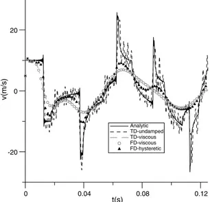
Figs. 8 and 9show, respectively, the results related to the vertical displacement and velocity at point A(25, 25, 0) at the

centre of the membrane. InFigs. 10 and 11, results at point B(12.5, 12.5, 0) obtained from the 3D analysis is compared with

the corresponding analytical solution (see [19,31]). A good agreement is observed between analytical and numerical

responses. The results obtained from the 2D analysis are not shown, since they are very close to the 3D ones.

With the purpose of observing the influence of the extended period on the response determined through FD analyses,

the membrane shown inFig. 6is analyzed again with different extended periods. Namely, the following pairs ofTpvalues

and sampling points were considered: Tp= 2.5 s and N= 2048; Tp= 1.25 s and N= 1024; Tp= 0.625 s and N= 512;

Tp= 0.3125 s andN= 256; andTp= 0.1563 s andN= 128. These values of the extended period correspond, respectively,

0 0.002 0.004 0.006 0.008

t(s)

-20 -10 0 10 20

v(m/s)

Analytic TD-HHT FD-hysteretic FD-viscous

Fig. 5. Velocity time-history at the free end of the rod under Heaviside-type forcing function and initial conditions prescribed in part of the domain.

Fig. 6. Square membrane under prescribed initial velocity field.

x

y z

L _L

0 0.04 0.08 0.12

t(s)

-0.1 0 0.1

u(m)

Analytic TD-undamped TD-viscous FD-viscous FD-hysteretic

Fig. 8. Displacement time-history at the center of the square membrane.

0 0.04 0.08 0.12

t(s)

-20 0 20

v(m/s)

Analytic TD-undamped TD-viscous FD-viscous FD-hysteretic

Fig. 9. Velocity time-history at the center of the square membrane.

0 0.04 0.08 0.12

t(s)

-0.08 -0.04 0 0.04 0.08

u(m)

Analytic TD-undamped TD-viscous FD-viscous FD-hysteretic

toh values of approximately 1.49·₁₀3_{%, 0.39%, 6.22%, 24.9% and 49.9%, respectively. The time reconstitution of the}

displacement at the centre of the membrane is presented inFig. 12.

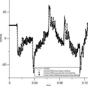
InFig. 13, the velocity time-history at the centre of the membrane, obtained by employing the Central Difference[29]

and the Fourth Order Finite Difference[30]explicit algorithms (TD analyses), is presented. The classic initialization

pro-cedure as well the initialization propro-cedure proposed here, were adopted. As in the case of the previous TD analyses, 1250

time steps of lengthDt= 0.1 ms and no damping were considered.

5. Conclusions

This work is concerned with the presentation and validation of a unified approach that enables one to compute the con-tribution of initial conditions in time- and frequency-domain analyses. Basically, the approach consists in expressing the initial conditions in terms of suitable pseudo-forces. As shown here, the method is quite general, i.e., frequency-domain equations are directly obtained from corresponding time-domain ones. The examples presented confirm its applicability and generality, encouraging its further extension to elastodynamics. In all cases analyzed, a quite good agreement with

the analytical solutions was attained (seeFigs. 2–5, 8–11). As observed inFig. 12, the correct choice of the extended period

Tpplays an important role in a reliable representation of the causality. A very short value ofTpbrings perturbations at the

0 0.04 0.08 0.12

t(s)

-10 -5 0 5 10 15

v(m/s)

Analytic TD-undamped TD-viscous FD-viscous FD-hysteretic

Fig. 11. Velocity time-history at the point B(12.5, 12.5, 0) for the square membrane.

0 0.04 0.08 0.12

t(s)

-0.1 0 0.1

u(m)

Analytic-undamped FD-hysteretic-Tp=2.5000,N=2048 FD-hysteretic-Tp=1.2500,N=1024 FD-hysteretic-Tp=0.6250,N=512 FD-hysteretic-Tp=0.3125,N=256 FD-hysteretic-Tp=0,1563,N=128

initial time due to previous time history, i.e. the causality condition is not verified; otherwise, ifTpis too long the analysis

cost will be increased.

On the other hand, the responses shown inFig. 13, obtained through TD analyses also indicate that the proposed

ini-tialization procedure can be adopted in the most general case of initial conditions. It is important to notice that the use of this initialization procedure can be very attractive from the computational point of view, since the inversion of the mass matrix in implicit time-marching schemes becomes unnecessary.

The Finite Element Method (FEM) was used here. Nevertheless, the pseudo-force method is independent of the numer-ical approach adopted and can be applied with other numernumer-ical methods, for instance, the Finite Difference Method (FDM) or the Boundary Element Method (BEM).

References

[1] P.K. Banerjee, The Boundary Element Method in Engineering, McGraw-Hill, New York, 1994. [2] K.J. Bathe, Finite Element Procedures, Prentice-Hall Inc., Englewood Cliffs, NJ, 1996.

[3] D.E. Beskos, G.D. Manolis, Boundary Element Methods in Elastodynamics, Springer-Verlag, 1987. [4] C.A. Brebbia, J.C.F. Telles, L.C. Wrobel, Boundary Element Techniques, Springer-Verlag, 1984. [5] E.O. Brigham, The Fast Fourier Transform, Prentice-Hall Inc., Englewood Cliffs, NJ, 1974. [6] A. Butkov, Mathematical Physics, Addison-Wesley, 1968.

[7] R.W. Clough, J. Penzien, Dynamics of Structures, McGraw-Hill, Berkeley, 1993.

[8] J. Dominguez, Boundary Elements in Dynamics, Computational Mechanics Publications & Elsevier, London, 1993.

[9] W.G. Ferreira, A.M. Claret, F. Venancio-Filho, W.J. Mansur, F.S. Barbosa, A frequency-domain pseudo-force method for dynamic structural analysis: nonlinear systems and non-proportional damping, J. Brazil. Soc. Mech. Sci. XXII (4) (2000) 551–564.

[10] A.P. French, Meca´nica Newtoniana, Editora Reverte´, Barcelona, 1974.

[11] H. Grundmann, E. Trommer, Transform methods-what can they contribute to (computational) dynamics? Comput. Struct. 79 (2001) 2091–2102. [12] D. Hall, Basic Acoustics, Krieger Publishing Company, 1987.

[13] H.M. Hilber, T.J.R. Hughes, R.L. Taylor, Improved numerical dissipation for time integration algorithms in structural dynamics, Earthquake Engrg. Struct. Dynam. 5 (3) (1977) 283–292.

[14] T.J.R. Hughes, The Finite Element Method: Linear Static and Dynamic Finite Element Analysis, second ed., Prentice-Hall, New Jersey, 2000. [15] L.E. Kinsler, A.R. Frey, A.B. Coppens, J.V. Sanders, Fundamentals of Acoustics, third ed., John Wiley & Sons, New York, 1982.

[16] L.E. Malvern, Introduction to the Mechanics of a Continuous Medium, Prentice-Hall Inc., Englewood Cliffs, NJ, 1969.

[17] W.J. Mansur, W.G. Ferreira, F. Venancio-Filho, A.M. Claret, J.A.M. Carrer, Time segmented frequency-domain analysis for non-linear multi-degree-of-freedom structural systems, J. Sound Vib. 237 (2000) 457–475.

[18] W.J. Mansur, D.J. Soares, M.A.C. Ferro, Initial conditions in frequency-domain analysis: the FEM applied to the scalar wave equation, J. Sound Vib. 270 (4–5) (2004) 767–780.

[19] P.M. Morse, K.U. Ingard, Theoretical Acoustics, McGraw-Hill, New York, 1968.

[20] P.M. Morse, H. Feshbach, Methods of Theoretical Physics, McGraw-Hill, New York, 1953.

[21] A.V. Oppenheim, R.W. Schafer, Discrete Time Signal Processing, second ed., Prentice-Hall Inc., Englewood Cliffs, NJ, 1989. [22] M. Paz, Structural Dynamics—Theory and Computation, fourth ed., Chapman and Hall, New York, 1997.

[23] J.G. Proakis, D.G. Manolakis, Digital Signal Processing—Principles, Algorithms and Applications, third ed., Prentice-Hall Inc., Englewood Cliffs, NJ, 1996.

[24] D.J. Soares, W.J. Mansur, An efficient time/frequency domain algorithm for modal analysis of non-linear models discretized by the FEM, Comput. Methods Appl. Mech. Engrg. 192 (2003) 3731–3745.

0 0.04 0.08 0.12

t(s) -20

0 20

v(m/s)

Analytic

Central Difference-classic starting Central Difference-pseudo-force starting Fourth Order Difference-pseudo-force starting

[25] W.T. Thomson, Theory of Vibration with Applications, first ed., Prentice-Hall Inc., Englewood Cliffs, NJ, 1973.

[26] A. Veletsos, C. Ventura, Efficient analysis of dynamic response of linear systems, Earthquake Engrg. Struct. Dynam. 12 (1984) 521–536.

[27] F. Venancio-Filho, A.M. Claret, Matrix formulation of the dynamic analysis of SDOF systems in the frequency domain, Comput. Struct. 42 (5) (1992) 853–855.

[28] J.P. Wolf, Dynamic Soil–Structure Interaction, Prentice-Hall Inc., Englewood Cliffs, NJ, 1985. [29] O.C. Zienkiewicz, R.L. TaylorThe Finite Element Method, vols. 1 and 2, McGraw-Hill, 1989.

[30] J.A.M. Carrer, C.J. Martins, L.A. Sousa, A fourth order finite difference method applied to elastodynamics: finite element and boundary element formulations, Struct. Engrg. Mech. 17 (6) (2004) 735–749.