SPECTRAL METHODS IN OCEANOGRAPHY WITH APPLICATIONS

Bolm Inst. oceanogr., S Paulo, 27(2):153-190,1978

SPECTRAL METHODS IN OCEANOGRAPHY

WITH APPLICATIONS*

PEDRO ALBERTO MORETTIN

&

AFRÂNIO RUBENS DE MESQUITA

Ins~ituto

de Matemática e Estat{stica e Instituto Oceanogpáfico

da

Univereidade de são Paulo

SYNOPSIS

This paper is a survey of the main spectra1 methods potentia11y usefu1 in Oceanography. These methods are app1ied to the ana1ysis of t ides, s easona1 variations and ocean geophys ica1 os ci 11a tions. Further topics on the Response Method, the Maximum Entropy method and Rotary Components are brief1y summarized. Examp1es of successfu1 app1i-cations are presented.

1 - I NTRODUCT I ON

This paper intends to be a survey of the main spectra1 methods potentia1-1y usefu1 in oceanography. Some practica1 prob1ems are discussed but they do not cover, of course, the range of a11 possib1e app1ications.Basica11y,

*-

This work was partia11y supported by Projeto FlNEP-IOUSP, Sub-Projeto n9 3 - Hidrodinâmica Costeira, and Fundação de Amparo

ã

Pesquisa do Esta-do de são Paulo (FAPESP).

- Paper presented at the 1977 Annua1 Meeting of the Amer.ican Statistica1 Association, August 15-18, 1977, Chicago, I11inois.

154 Bolm Inst. oceanogr., S Paulo, 27(2), 1978

there are three types of phenomena that appear in physical oceanography: first, those which present known frequencies and phases and we are interested in their amplitudes; secondly, those which possess known frequencies, and the interest is to determine phase and amplitudes and finally there are those phenomena for which frequencies, phases and amplitudes are unknown. According to other classification the hidrodynamical ocean processes are as-sumed to be of planetary scale (sections 3 and 5), medium scale and micro-scale, eventhough there is not a precise separation between these scales. Processes of medium and micro-scale are further discussed in Mesquita

&

Morettin, 1976.

The plan of the paper is as follows: in s'ection 2 we describe some gener-al spectrgener-al methods; in section 3 we present the fundamentaIs of tide angener-aly- analy-sis and results of a simple analyanaly-sis of a tidal record are given. An appli-cation concerning seasonal variation is given in section 4 and in section 5 some preliminary analysis of GATE (GARP ATLANTIC TROPICAL EXPERIMENT) data is discussed.

2 - GENERAL SPECTRAL METHODS

Let X = {X(t,w):teT,WEn} be a real-valued stochastic process, where for each tET, X(t,w) is a random variable defined on the probability space (n ,A, p) • Usually we take T= Z= {O ,±l ,±2, ••• } or T= R, the set of real numbers • For fixed w we have a reatization~ trajectory or sampte function of X. The

set of alI these realizations is the enserrible. A problem which arises in practical situations is the determination of the ensemble. Suppose, for ex-ample, that we are interested in measuring wave heights in a given area. If an instrument is attached to a buoy and thrown in a point of this area, we

/

will have observations of a time series, which is part of a realization of the processo If the buoy is thrown in a different point we will observe an-other realiza~ion of the processo It is therefore necessary to stipulate the

MORETTIN & MESQUITA: Spectral methods: oceanography

155

We will indicate by 1J (t) = E [ X( t ,w) ] the expected value of X and by

C(tI,t2) the auto-covariance function of X, defined by

11(t) = E[X(t,w) ] =!xdF(x,t), (2.1)

(2 .2)

respectively. Here, F(x,t) = P(X(t) ~ x) is the distribution function of the

random variable X(t,w). lf tI = tz we have the variance of X(t,W). We will

omit the dependence on w and write simply X= {X(t), tEZ}.

2.1 - STATlONARY PROCESSES

Let T= Z and suppose we have now a vector-valued stochastic process

X(t) _,... =

X (t) p

, tEZ, (2.3)

with p real-valued components. We say that X(t) is weakly stationary or

second-order stationary if

(i) 11· (t) = E [ X. (t)] = ll.,

J J J

(ii) Cjk(t+T,t) = Cov{Xj(t+T), Xk(t)} = Cjk(T),

156

Bolm Inst. oceanogr., S Paulo, 27(2), 1978

for t,T E Z and j,k = 1,2, ••• ,p. Without 10ss of generality we assume that

~. = 0, in such a way that the

cross-covariance function

C.k(T) of X.(t)

J . J J

with Xk(t) can be written

C.k(T) = E[X.(t+T)X. _{J J --k} (t)] _, (2.4 )

fort,T E Z and j,k= 1, ••• ,p. lf j= k we have the

auto-covariancefunctionof

X. (t).

J

lf we can assume that

00

E

I CJ.k(T)

1<

00, j,k= 1, ••• ,p,

T= -00

(2.5)

then we define the

second-order spectrum

of X.(t) with _{J .}

x.

_-K (t) by

(2.6)

for -00 < À < +00, j,k= 1, ••• ,p. lf j= k, f .. (À) is the

(power) spectrum

of

JJ

X. (t) at _J

frequency

À and if j=l k , f .k(À) is the _{J .}

cross-spectrum

of X. (t) with _J

Xk(t) at À. Expression (2.5) is a mixing condition in the sense that Xj(t+T)

and Xk(t) become 1ess dependent as ITI~. fjk(À) is bounded, uniformly

con-tinuous and of period 2TI; moreover,

(2.7)

Since fjk(À) is complex it can be written

MORETTIN

&

MESQUITA: Spectral methods: oceanography ₁₅₇

The real part of f _jk (À) _' c. (À), is ca11ed the _Jk

co-spectrum

and the imr _.

aginary part q. (À) is ca11ed the

quadrature spectrum

(or

quad-spectrum).

Jk

8jk(À) is the

phase

_{spectrum and f jk (À) is the}

ampl i t ude spectrum.

A

quantity of interest in the ana1ysis of pairs of time series is the

coherence,

defined by

(2 . 9)

Pjk(À) is the ana10gue of the corre1ation coeffi ci ent between two randçm

variab1es and measures (in the fre~uency doma in) the extent of linear

re-1ationship between Xj(t) and ~(t). It can be proved that O ~ Pjk(À) ~ 1 .

Linear here shou1d be understood in the sense that there is a linear filter

acting on Xj(t) and producing ~(t) (see discussion be1ow) .

Let us consider the case of a sing1e series X. (t) for a moment. A theorem

J

by Bochner states that there is a non-decreasing, bounded function F. (À) such

J

that

J

'IT iÀT

C .. (T)

_JJ

=

e

dF.(À),TEZ.

_'IT J (2.10)

This function F.(À) is the

J

spectral distribution function

of the series

X.(t) and determines a

spectral measure

F.(~), which can be written

J ' J

d c

F . (~)

=

F. (~) + F. (~) •

J J J

and _F:(~) are, respective1y, the

discrete

and the

J

and they are such that

"\ LA p .. (À_{k ) ,}

I\kELl JJ

Lf. .

(À)dÀ;

Ll JJ

(2.11)

continuous part

of

(2.12),

158

Bolm Inst. oceanogr., S Paulo,

27(2) , 1978

p .. (À_{k) is the}

spectral function

JJ and f .. JJ (À) is the

spectral density function

or simply the spectrum~ given by

(2.6)

if

(2.4)

holds (wit~ j = k). It follows

that

e ..

(T) can bewritten

JJ

(2.14)

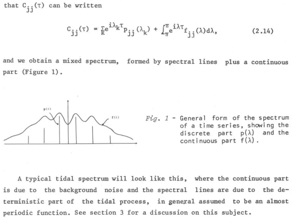
and we obtain a mixed spectrum, formed by spectral lines plus a continuous part (Figure 1).

p (»

Fig. 1 - General form of the spectrum

of a time series, showing the discrete part p(À) and the cont i nuous pa rt f (À) .

A typical tidal spectrum will look like this, where the continuous part is due to the background noise and the spectral lines are due to the de-terministic part of the tidal process, in gene~al assum~d to be an almost

periodic function. See section 3 for a discussion on this subject.

2.2 -

THE BISPECTRUM

Let

e

_{J . . . (tl,t2,t3) be the cumulant of order 3 of the p vector-valued}

1] 2]3 d

time series != {~(t),tEZ}. Assume that ~ is 3r order stationary. that is. the finite-dimensional distributions of X up to order 3 are invariant under time translations. Then it fol1ows that

and if E[X.(t)J= 0, j= 1 ••••• p, then

J

e . . .

_J1]2J3 (Tl.lZ) =E[X. (t)X. (t+Tt>X. (t+T2)]

] I J2 J3

(2.15)

MORETT IN & MESQUITA: Spectral methods: oceanography 159

where jl,j2,j3 = 1, ••• ,p. lf P is any permutation of the indices 1, 2 and 3,

then it is a1so true that

(2.17)

For further details on cumulants~ see Bri11inger, 1975, Chapter 2.

If

(2.18)

the

bispectrum

of X is defined by

(2.19)

for -00 < Àl,À2 < +00, and this is bounded, uniform1y continuous and periodic

with period 2TI with respect to Àl and À2. By (2.17) we have

(2.20)

and if the components of ~ are real, then

(2.21)

A1so, in the case of the bispectrum of a sing1e series X.(t), we have J

(2.22)

If x. (t)

:f

X. (t)

:f

X_k (t) we call f .. k(Àl ,À2) the

trivariate bispectrum

1 J 1J .

of x.(t), X.(t) and ~(t); if X. (t)

=

X. (t)

:f

~(t), f. .k (Àl ,À2) is the

1 J 1 J 11 .

cross-bispectrum

of x.(t) and _{1 ~(t)} ; finally, if X. (t) ₁

=

X. (t)

=

~(t),

160 Bolm Inst. oceanogr., S Paulo,

27(2), 1978

f .._1.1.1. .

0..1

,À2) is the auto-bispeatrum of X. (t). We can also write f. . . (Àl,À2) _{1. J1]2J3} as f . . . (Àl,À2,À3), with the understanding that Àl+À2+À3= 0,

J 13 2J 3

3

that is, the bispectrum has support only on the manifold.L À.= _{1.=1 1.}

°

of the (Àl,À2,À3)-space.

lf (2.18) is not satisfied we can formulate a general theory for polyspectra

(Brillinger

&

Rosenblatt, 1967; Gasser, 1972).

The records of ocean waves, in a given position, may be considered as realizations of Gaussian stationary processes. For these processes the spectrum is adequate to analyse their probabilistic structure. It is known that for Gaussian process the cumulant spectra of order greater than two vanish. Therefore, the bispectrum (and polyspectra of higher order) can be useful to detect deviationsfroma Gaussian processo The complexity of ocean waves, for example, makes necessary to consider moments greater than 2 and, in consequence, higher-order spectra. On the other hand, there have been relatively few

appli-cations of polyspectra, mainly due to difficulties of interpretations, time and computer work progrannning. Brillinger, 1965 says: "Experi ence wi th rea 1 random variables indicates that higher order moments are not efficient esti-mates of sc i ent i f i ca lly re I evant pa rameters; consequent ly as the s pec i f i cat i ons of stochastic processes become tighter, polyspectra are likely to prove less pertinent in a similar manner."

Applications have been restricted to auto-bispectrum. Hasselmann et al.,

1965, have analysed the bispectrum of wave records at a single station.

. nd rd

Brillinger

&

Rosenblatt, 1967a, have cons1.dered 2 and 3 order spectra of the sunspot numbers series.

2.3 - HOMOGENEOUS PROCESSES ON A SPHERE

Let X= {X(P,t):PE82,tEZ} be a real-valued stochastic process defined on the unit sphere 82 oflR3• We assume that X is continuous in quadratic mean (q.m.), with finite mnments of alI orders and (~eakly) stationary with

re-spect to t and homogeneous with rere-spect to P, that is

( i) E{X(P,t)} = constant,

(ii) Cov{X(P,t+s), X(Q,s)} = R(8,t),

r.

MORETTIN & MESQUITA: Spectral methods: oceanography 161

where 8 is theangular distance between P and

Q.

We assume that the mean (2.23) is zero. It then follows that

with

00 n X(p,t) = l: l:

n=O j=-n

Z • (t) Y • (p) ,

nJ nJ

Z .(t) =

fs

X(p,t)Y .(P)dP,

nJ 2 nJ

(2.25)

(2.26)

where dP is the measure on S2 and {Y., -n _{( nJ - -}< j < n} are the spherical har-monics of order n>"O. In (2.25) the series ts assumed to be convergent in

q.m. and the integral l.n (2.26) is a stochastic integral in the q.m. sens-e. See Yaglow, 1961, for a fu11 treatment of the above expressions. See a1so Roy, 1976.

The process Z .(t) is such that nJ

{

}

_f

TI ih

E Z .(t+s)Zmk(s) = _nJ

o

_nm O.k _{J -TI} e dF _n

(À),

and the covarl.ance function R(8,t) is given by

where P (.) _n

R(8,t) =

(4TI)-ln~O(2n+l)Pn(COs

8)

f

TIeiXtdFn(À) , -TI

are the Legendre polynomials of degree n and

(2.27)

(2.28)

{F _n (À)} is a sequence of real, bounded, non-decreasing functions.

distribution function of X.

F (À) is the spectral _n

App1ications of stochastic processes on a sphere have been done by Jones, 1963 and Cohen

&

Jones, 1969. They have applied the methodo1ogy of this section to the problem of meteoro1ogica1 forecasts.

2.4 - FILTERING, SAMPLING AND ALIASING

band-162

Bolm Inst. oceanogr., S Paulo, 27(2), 1978

pass filter in order to isolate the most important tidal components.

By a filter we mean a mechanism ~whic h transforms a time series X(t) in

another time seriesY(t) and we indicate this by Y(t) =

1

[X(t)] •

-J

is a

Zinea:t> fi

l

ter

if:

(ii) if Y(t) = 3"[X(t)], then Y(t+T) = 1[X(t+T)] •

Property (i) gives the liriearity of

si

and (ii) gives the so-called

time-invananae

of'Í. Of special importance are the filters

(2.29)

for stationary processes X(t) and

y(p) _{= (2TI)J O} _1 2TI TI

Ia

_{h(8) X(Q) sen 8d8d<j>,} (2.30)

for homogeneous (time-independent) processes on a sphere, 8 and <j> being the latitude and longitude of Q. The filters (2.29) and (2.30) are comp1etely

determined by their respective

transfer funa tions

(2.31)

and

(2.32)

where P_{À (.)} is the Legendre polynomial. In case (2.29), if fXX(À) and fyy(À)

are the spectra of X(t) and Y(t), respect ively, then the simple relation

fyy(À) = IH(À) 12 • fxx(À) holds.

Suppose now we have a continuous, stationary series {X(t) , ~t<~} and

we sample it at j~t, jEZ, ~t>O. We obtain the series

MORETT IN & MESQUITA: Spectral methods: oceanography ₁₆₃

Through this sampling procedure some harmonics of the spectral decompo-sition of X(t) cannot be distinguished. This is the

aZiasing

phenomenum and if we denote by f(À) and f~t(À) the spectrum of X(t) and X~t(j), respective-ly, then it can be shown that

À . . [-TI TI ]

For any ~n the ~nterval ~t'~t ' the are called the

aZiases

of À. The frequency

f . À 2krr

requenc~es +

Lrt:'

rr (. d.

~t ~n ra ~ans per

(2.34)

k= ±l, ±2, • ••

unit of time) is called the

Nyquist frequency.

lf frequency is given in cycles per unit of time, the Nyquist frequency is 1/2~t. If ~t is small in such a way that f(À) ~ O

for IÀI > :t then

f~t(À)

and f(À) will be es-sentiall; the same. On the other hand, if there is no interest in f(À) for

1

À

1

> :t' thenwe can avoid aI ias ing through the applications of a low-pass filter, which attenuates or eliminates the energy at high frequencies. For details on the effect of aliasing in the case of stochastic processes on a sphere see Hannan, 1966.

The problem of aliasing also appears in connection with bispectrum . lf we have two continuous series X(t) and Y(t), . for example, and

À~x)

- Ix' À(y) - TI are the respective Nyquist frequencies, then the cross - bispectra of

N ~y ,

the continuous series and of the sample series will be essentially the same

if _{the f YXX(Àl,À2)}

~

O for \Àl\ >

À~x)

and

1\1

>

~y).

Under regularity conditions, it can be shown that

3

for~ À.

j =1 J

f

(~t) (À À À) ~f (À 2rrj 1 À2 2TIh À3 + 2TIj 3)

. YXX 1, 2, 3 = L. 'YXX 1 + ~t' + ~, ~t'

=

O

(mod 2TI), the sum extended over alI J_a such that

3 2TIj a L

0..2

+

---xi:)

a=l O and ~x= ~y= ~t.

(2.35)

For practical aspects of computations of the bi-spectra see Brillinger

&

Rosenblatt, 1967a and Gasser, 1972. To give an idea, for one series X(t), the bi-spectrum f XXX{Àl,À2) is computed ~n the triangular area of vertices (O O O) (TI O -TI) and (TI,TI,-TI), ';n the case Àl + À2 + À3 = O

" , " .L

164 Bolm Inst. oceanogr., S Pa~lo, 27(2), 1978

2.5 - ESTIMATION PROCEDURES

In this section we restrict our attention to the problem of estimating 'spectra and bispectra. There are basically two approaches for estimating spectral parameters. The first uses estimates which are obtained through a smoothing of the sample covariance function. The second uses estimates which are weighted averages of periodogram ordinates.

Suppose we have observations X(t) , t= 1, ••• , N of the p vector-valued

process (2.3). Define the vector (pxl) of

finite Fourier transforma

(2.36)

2'!TV

f or -00 < À < +0:>. Vsuallythis is computed for frequencies

Àv=

N'

for

_ [N-l 'J ₂ < _- V _-<

r~

_L2

J.

Let E[X(tfl = _~

°

and f (À) be the matrix of spectra

f. k(À) , j ,k= 1, ••• ,p. Under regularity conditions (Brillinger, 1975) the random

v!riable

~

(N) (À) has an asymptotic distribution which is a muI tivariüte

com-plex normal distribution NC(O,f(À», if À+ O,'!T. lf À=

°

or À= '!T, the

asympp -t o-tic dis-tribu-tion is a N (O,f(À».

(N) p

-Let d j (À)bethe j-thcomponent of

~(N)(À)

and define t,he

aross-pePiodogram

of the series Xj(t) with the series ~(t) by

lf j= k we have the

pePiodogram

of X.(t) given by

J

(2.37)

(2.38)

lt can be proved that I

~~)(À)

is an asymptotically unbiased estimator of

JJ

f .. (À), but it is not consistent, since its variance is (asymptotically)

JJ 2 (N)

equal to f..(À), for À; O,'!T and 2f~.(À), for À=

°

or À='!T. Moreover, 1.. (À)

JJ J J J J .

has an asymptotic distribution proportional to a chi-square variable with 2

degrees of freedom, if À; 0, 7T and proportional to a chi-square variable with

MORETTIN & MESQUITA: Spectral methods: oceanography 165

Let ejk(T) be an estimate of the cross-covariance function Cjk(T) defined by

-1 N-T

N

r

X.(t+T)X. (t), T= O,1, ••• ,N-1

t=1 J -K

ekj(-T), T= -1,-2, ••. ,-N+1 (2.39)

0, ITI >N.

Let WM(T) be a sequence of weights such that:

(2.40)

(iii) WM(T) = 0, for ITI > M.

The function WM(T) is ca11ed a

lag window

and its Fourier transform

(2.41)

is ca11ed a

speatral window

and has the properties:

(2.42)

There are many windows used in practice, such as the Bart1ett, Tukey,

Parzen windows, etc. See Jenkins

&

Watts, 1968 for detai1s.

lf we co11ect the Cjk(T) in the pxp matrix C(k), we define the

smoothed

aovarianae estimate

of ~(À) by

166 Bolm Inst. oceanogr., S Paulo, 27(2), 1978

lt can be seen, from the convolution properties of the Fourier transform and using a Riemann approximating sum for an integral (Koopmans, 1974, p. 267), that t (À) can be written in the asymptotically (in distribution sense)

-1

equivalent form

t

(À) =

-2

[!]

2 (N)

E

N

1 K(À-À).

I

(À),

_[-J

v

-

V

v--

-2-(2.44)

where Àv =

2;V

and K(À) is a symmetric, periodic, rea1-valued weight function

for which LK(À)= 1. Here !(N) (À) =

[l~~)

(À)] is the matrix of

cross-periodograms (2.36). Estimators given by (2.43) are called

smoothed periodogram

estimators.

The estimators (2.42) and (2.43) are asymptotically unbiased and,

under regu1arity conditions on M, N and K(À) , they have, asymptotically, a

distribution which is a constant mu1tip1e of a chi-square variab1e with r

degrees of freedom. The parameter r is ca1led the

equivaZent degrees

of

freedom

of the estimator and depends on K(À) , since K(À)

~

2nW (À). lf we

n N M

use (2.42), then r=

_{N/f WM}

2_{(À)dÀ and if we use (2.43), r= 2/EK}2_{(À ).}

-n

v

As estimates of the coherence Pjk(À) and of the phase 8_{jk(À) we take}

[Fjk(À) ] PJ'k(À) =

-[ _{I . ,} ~ _{(À) fkk(À)}

-11/2

JJ

-(2.45)

and

(2.46)

where êjk(À) = Re Fjk(À), qjk(À) = Im tjk(À) and tjk(À) is given by (2.42) or (2.43).

MORETT iN

&

MESQUITA:

Spectral methods: oceanography

₁₆₇

It is given 'by

r - r

log

b

+ log f(À) < log f(À) < log

ã

+ log t(À), (2.47)

where a and b are obtained from the tables ofax2(r) by

y being the confidence coefficient. The constant width of the interval is

b

log

ã'

See Koopmans, 1974, for the expressions for the confidence intervals for the coherence and phase.

Turning to the bispectrum, define the third-order periodbgram by

(2.48)

where Àl + À2 + À3

=

O. As an estimate of the bispectrum we take'the weighted periodogram

tt~

j 0'1 ,À2 ,À 3) =ff::fWM(À l-aI ,À2-U.2 ,À 3-(3)

It~

j (aI ,a2 ,(3) o(al+a2+a3) dalda2da3, (2.49)

I 2 3 I 2 3

where WN(.) is a continuous weighting function and Ô (.) is the Dirac function.

For computations, (2.48) can be written in a form similar to (2.43). For details, see Brillinger

&

Rosenblatt, 1967. The estimate (2.48) is asymp-totically unbiased off minor submanifolds and asympasymp-totically normally dis-tributed as N + 00.

A further aspect that deserves attention 1n the estimation of spectra and bi-spectra is the problem of compZex-demoduZation. Let X(t) be a real-valued series and consider

x

(t)

o (2.50)

168 Bolm Inst. oceanogr., S Paulo, 27(2), 1978

the bandwidth of L, then an estimate of the spectrum of X(t) in ÀO ± ~À is given by T- l

J~~IXo(t)

12dt, where T is the 1enght of a record of X(t) from

t= tI up to t= t2. As an estimate of the (trivariate) bi-spectrum of Xl (t) , X2(t) and X3(t) we take

X "\ (t) X "\ (t) X (t) ,

1 , 1 \ 1 2 , 1 \ 2 3,À3 (2.51)

where Àl + À2 + À3 = O, N is the number of avai1ab1e va1ues of the comp1ex demodu1ates and X. "\.(t) is the comp1ex demodu1ate of X.(t) at frequency

].,1\1 1

À., i = 1,2,3. An advantage of this procedure is that we can obtain the

esti-1

mated cross-spectrum at the same time:

-1 N

=

N L X , (t)X , (t),

t=l 1,1\1 2,1\2 (2.52)

Àl + ~ . 2 = O. For detai1s, see Godfrey, 1965 and Tukey, 1961.

3. THEORETICAL AND REAL TIDES

Newton introduced the concept of the equilibrium tide (the tide that wou1d have been produced if the rigid and spherica1 earth were covered entire1y by the oceans) and this has been used as the basis for 1ater deve10pments 1n tida1 theory byLap1ace, Darwin, Doodson (1921) and Cartwright & Edden, 1973. In real tides, . as measured by tide gauges at a fixed point on earth, the equilibrium is never attained and the record tidal wave is a superposition of effects such as the revo1ution of the "fixed point" through the deformed water surface (by the tida1 tractive forces of the moon and the sun) from the spherica1 shape, the modification of the deformed water surface de-termined astronomica11y by the moon and sun positioning re1ative to the earth, sha110w water effects, radiation effects, atmospheric inf1uences and others.

MORETTIN

&

MESQUITA: Spectral methods: oceanography 169

to the orbits of the moon and the sun (frame of reference put on earth) and in the Equilibrium Theory of T~des • ~ °t ~s o d escr~ °b d b e y the t~de o generating

potential (Munk

&

Cartwright, 1966) V(P,t)= V(e,~,t) given by

(3.1)

which can further be written in the form

v(e,~,t)

(3.2)

In equation

(3.2),

e and ~ are the colatitude and longitude of the point P on the earth's surface; t ~s the time, a is the radius of the earth and ~

is its mass; eL and ~L are the colatitude and longitude of the moon, ~ its distance from the centre of the earth and ~ its mass. Similar terms with the subscript S refer to the sun. The terms ym are the spherical harmonics, _n defined by

) !

j

1/2 P Im I ( e)

im~

r--+-~)-.. _{• n} co s e

pm being the associated Legendre functions n

(3.3)

(3.4)

170 Bolm Inst. oceanogr., S Paulo, 27(2), 1978

periodical parameters of the orbits of the moon and the sun used for time description of (eL'~L) and (eS'~S) are:

the

T= the lunar time

s= the mean longitude of the moon h= the mean longitude of the sun p= the longitude of the lunar perigee

N'= the negative of the longitude of the ascending node p'= the longitude of the perihelion.

Here, p' completes one revolution in 20,900 years, N' 1.n 18.61 years, p

1.0 8.85 years, h in one year, s in one lunar month. lf we write (3.1) as

V(P,t) = v(eL'~L,t) + v(eS'~s,t), then the resulting expansion of the two terms in the right hand-s ide of this equality in terms of the variables (3.5)

are given as a sum of cosines and sines of

iT + js + kh + lp + mN' + np' ,

where the weights {i, j, k, I, m, n} are th~ Doodson' s numbers and they varie from -6 to +6 individually (Godiri, 1972). A combination of integers

{i, j, k, 1, m, n} characterizes a

constituent

with

frequency

. . .

.

À

=

ii

+ js + kh + lp + mN' + np' (3.6)

of the tidal spectrum and in the Harmonic Method of tidal analysis the search for its phase and amplitude is the prior objective.

As already mentioned, modifications of the shape of the disturbed sea leveI, due to the action of the generating tidal potential described by (3.1) are much slower than the rate with which the observing point P= (e,~) is

displaced, so P "moves" through the disturbed sea leveI.

MORETTIN

&

MES QUITA: Spectral methods: oceanography

171

majority of ports) the recording of a predominant semi-diurna1 tide which 1.S

representat ive of a day sample of the "shape" of the tide generating po-tential. lts spectrum would have a predominant 1ine (M2 group of

constitu-ent s) at À=

2i

+ Os + Oh + Op + ON'+ Op' ;'0.08 cycles/hour, p1us other minor contributors.

A

set of dayly samples covering the period of one lunar month

(s is associated with this period of approximate1y 28 days) would have in each day record a predominant semidiurnal variation, but with modulated ampli t udes from one da)' to another, due to the variations of the "shape" of the water leveI (shape of the tide potential at P= (8,~», as the moon has

compl et ed during this period one orbit lenght and the earth about 1/12 of its path ar ound the sun. lncreasing the number of samples other features of the t ide generating potential are addedto the semi-diurnal wave carrier and t hey can be analysed by Fourier methods.

Usua lly it is assumed that the spectrum of V( t) is a 1ine spectrum . Munk & Cartwright, 1966, noticed however that the spectrum of tida1 records consis ts of peaks energing from a continuous spectrum. The continuous part is due to background noise, particularly in low frequencies.

Hence, a reasonable model is the following. We assume that a tidal record is a superposition of a strong deterministic process p1us a weak random processo Specifically, let E (t)astationary, ergodic process, withmeanzero and covar iance function C (T). Let x(t) be a non-random, real function of t,

EE

for wh i ch the Wiener covariance function

C (T) = lim

iT

L~

x (t)x(t+T)dt xx T-+OO

exists and it is finite for every T. Assume also that

lim-f.r

L~

x(t+T) E(t)dt

t-+OO

o

(3.7)

(3 .8)

where the l imits are in q.m. sense. lf Z(t) is the tida1 height, then write

172

Bolm Inst. oceanogr., S Paulo, 27(2), 1978

-00 < t < +00. It fo11ows that

(3.10)

and Z(t) wi11 have a spectra1 distribution function (in Wiener's sense)

F _Z (~)= F _X (~) + F _E (~). (3.11)

Usua11y, x(t) is assumed to be an a1most periodic function of the form

n D..t

x(t)= .i: C.e J ,

J='""n J (3.12)

and E(t) is assumed Gaussian, in such a way that the spectrum of E(t) is continuous and the spectrumof x(t) is discrete.

In the notation of section 2.1,

(3.13)

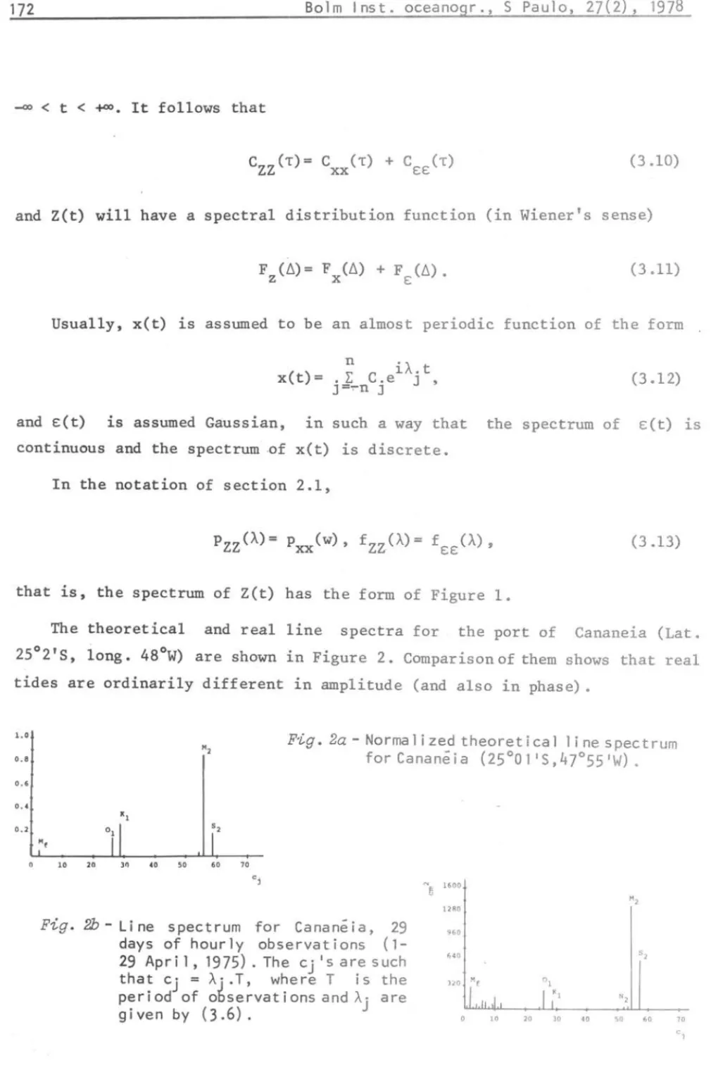
that is, the spectrum of Z(t) has the form of Figure 1.

The theoretical and real 1ine spectra for the port of Cananeia (Lat. 25°2' S, 10ng. 48°W) are shown in Figure 2. Comparison of them shows that real tides are ordinari1y different in amplitude (and also in phase) •

1.0

0.8

0.6

o .•

0.2

F'ig . 2a - Norma I i zed theoret i ca I I i ne s pec t rum

for Cananéia (25°01 IS,47°55IW).

10 20 lO '0 50 60 70

Fig. 2b - Li ne spectrum for Canané i a, 29

days of hourly observat ions (1-29 Apri I, 1975) . The Cj IS are such

that Cj = Àj.T, where T is the period of observationsa ndÀj are given by (3.6).

N

E

u 1600

1280

960

640

3LO

52

M f

0,

K,

MORETTIN & MESQUITA: Spectral methods : oceanography 173

For the theoretical spectrum we followed Godin, 1972. The real 1ine spectrum is a single use of (2.35) on a 29 days record lenght. Sampling intervals of the tidal records were so to give a 0.5 cy /hour Nyquist frequency ,but for Figure 2 only 75 Fouri er components were taken. In Figure 3 we have

10000

LP

1000

so

'ti 100

Ilo II

"-N

e

10

>-..

...

•

1

I:

li

C

&: lo< 0.1

•

I:

(01

0.01

o 5 10 15

cpd

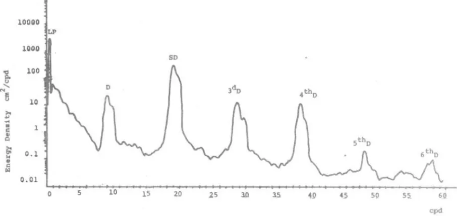
Fig. 3 - Estimated spectrumforCananéia,withone yearofhourly observations.

the spectrum of Z(t) given by (3.9), obtained from a record 1enght of one year, using a smoothed procedure and a FFT algorithm (Franco

&

Rock, 1971), with 8,192 digitized points.

The higher order peaks obtained are not direct1y due to the tidal po-tentia1 but to the distortions of the tidal wave as it 100ses energy at the shelf areas. Open ocean records are freer of thes'e effects. The higher order f requenc1es . (3 rd , 4th , etc, d' 1urna 1 f requenc1es ' ) are t e resu ts o t e h 1 f h important tidal constituents M1,Kl,M2,S2, etc (Doodson, 1957) and they can be expressed as sums and differences of these.

The record 1enght is fundamental for separating the tida1 constituents predicted by (3.1) from the semidiurna1 wave carrier. Two constituents are considered res01ved if

174 Bolm Inst. oceanogr., S Paulo, 27(2), 1978

where N is the number of digitized values of the record and Ôt is the sampling intervalo

Some of the longest records (approximately200 years) are reported in Cartwright, 1971, but even these are insufficient to analyse for

p' .

Tidal analysis of short records (7 days) for some constituents is given in Franco, 1964.

The aliasing phenomenum is not often seen in tidal analysis as Ôt= 1 hour (standart sampling interval normally adapted for records already instru-mentally fil tered for waves, swells and other higher frequencies effects) is sufficiently small for most of the records. However when shallow water com-ponents are small but necessary for prediction purposes (as seen in Figure 3, a great portion of the tidal energy is at frequencies higher than those of the group of semi-diurnals) aliasing can be used to one' s advantage as in Horn, 1960.

Estimates of the spectra for every port may be different for many reasons, but 1n alI cases they are based upon the same frequencies À determined by (3.6). The phases of the constituents may alI be related, for every port, to one particular instant of time (and meridian) from when the time of s,h,p,N' and p' are related (Meus, 1962). With both phases and frequencies determin-istically given by astronomy, the estimates of the (real) tidal spectrum are mainly concerned with the amplitudes of the tidal constituents and the

de-termination of real phases as they are also of practical importance. ~

The determination for the spectral bands are influenced by the unavoida-ble presence of noise and its contribution to the spectra often interferes 1n the separation of the spectral lines (Munk & Hasselmann, 1964).

Tidal records are also the registrar of other non .tidal effects, such as atmospheric pressure and solar radiation. Analysis of tides giving a broad look to the matter 1S found in Munk

&

Cartwright, 1966. In this approach, records are assumed to be given by

(00 roo(oo ) ( ') d'

MORETTIN

&

MESQUITA: Spectral methods: oceanography

₁₇₅

where W(T), W(T,T'), ••• are the impu1se functions of the loca1ity. Th i s new approach nntivated recent analises by Cartwright & Tay1er, 1971 and Car t wr i ght & Edden, 1973, 1eading to more accurate va1ues of the theoretica1 tida1 con-stituents. Formula (3.15) can be written as

00

Z(t)= L: (3 . 16)

j=l

where W.(t1, ..• ,t.), j=1,2, •.• are assumed to be symmetric ~n i ts arguments.

J J

The Fourier transform of W.(t1, •.• ,t . ) is

J J

(À À)

f

00

f

00 ( , -i(À 1t1 + ••• + À. t·)d

W. 1, ... , . = .•• w. t1, ... ,t.;e J J tI

J J -00 -OOJ J

• •• dt.,

J

(3 . 17)

ca11ed the j-th transfer function or admittances. The prob1em that a r ~se s is

the estlination of these functions. We refer to the expansion (3.16) as a

VoZterra functionaZ expansion

(cf. Bri11inger, 1970; 1975, and Gasser, 1972). Usua11Y ' a few terms of (3.16) wi11 be sufficient. Munk

&

Cartwright, 1966, consider the linear term for tida1 ana1ysis of Hono1u1u and the linear and quadratic terms for the portof New1yn. Consider, therefore~

N

Z(t) = L:

ft ···ft

W.(t1, ••• ,t.)V(t-t1) ••• V(t-t.)dt1 ••• dt . (3 .18)

j =1 1 j J J J J

or the discrete ana1ogue, with the integraIs rep1aced by sums.

Under certain regu1arity conditions on V(t) and assuming that w. (t I, ... t.).E:

J J

L1(Rj,mj,~j),

it fo11ows that the Vo1terra expansion (3.16) exists with probability oneandW.(À.lo ••. ,À.) € LI. Here, lBJis the Borel field on:JRI

. J J .

and llJ is the Lebesgue measure in R J . Moreover, if V(t) has the spectral

representation

176 Bolm Inst. oceanogr., S Paulo, 27(2), 1978

then the spectra1 representation of Z(t) is given by

Z(t)

.... 1:J"l

N e iÀt

f ...

!

W.(À1, ... ,À.)dU(À1) ... dUO,.).

J=l 1\ À1+ •• À.=À J J J

J

(3.20)

For practica1 purposes the weights W. are assumed to be different from

J

zero on1y for integral va1ues of t, in such a way that (3.18) can be written as a sumo

The cumu1ant spectrum of order k of Z(t) can be computed (see Theorem 2.10.1 of Bri11inger, 1975) and in particular the cross-bispectrum between Z(t) and V(t), whieh is used for estimating W2(Àh À2) •

We note that V(t) does not have to be the tida1 potentia1; other input functions are used, such as pressure, solar radiation, etc. For details, see Godin, 1972 and Munk

&

Cartwright, 1966.

For the identification of the admittances W. we further assume that the

J

drived inputs are Gaussian. This is usefu1 because (Gasser, 1972):

(i) structures beyond the spectrum are introduced;

(ii) Gauss inputs are sufficient for time-invariant system identifi-cation;

(iii) Gaussian processes can be easi1y generated by computers.

It follows that Wl(Àl) and W2(Àl,À2) can be estim,ated by

(3.21)

and

MORETTIN

&

MESQUITA: Spectra1 methods: oceanography 177

respective1y, where tZV(Àl) is the estimated cross-spectrum between Z(t) and V(t) and t vvZ (Àl,À2) is the estimated cross-bispectrum between Z(t) and V(t); tVV(Àl) is the estimated (auto)-spectrum of V(t). For the estimation of W_j in general see Bri11inger, 1970 and Gasser, 1972.

A measure of corre1ation between Z(t) and V(t) 1S given by the estimated

coherence

(3.23)

After expanding V(t) in Greenwich coordinates and substituting 1n (3.16) we obtain the practica1 scheme of the Response Method, given by

Z(t)=

L

r w k c (t-k~T) +

E E

wnn'kk' c (t-k~T).C, (t-k'~T) + •••

R n n n kk' nn' n n

(3.24)

Besides the estimation procedure suggested above for the W., we can

J

estimate the wnk ' etc by 1east squares and then estimate the wj by Fourier

transforming. In (3.24) the constants c are determined by the position of _n the moon or of the sun. The fitting of (3.24) to the actua1 observations 1S eva1uated through the prediction variance, which for the linear term is given by

Var [Z(t) - kr w kC _{,n n n} (t-k~T) ] • (3.25) For detai1s see Munk

&

Cartwright, 1966.

4. SEASONAL VARIATIONS

178 Bolm Inst. oceanogr., S Paulo, 27(2), 1978

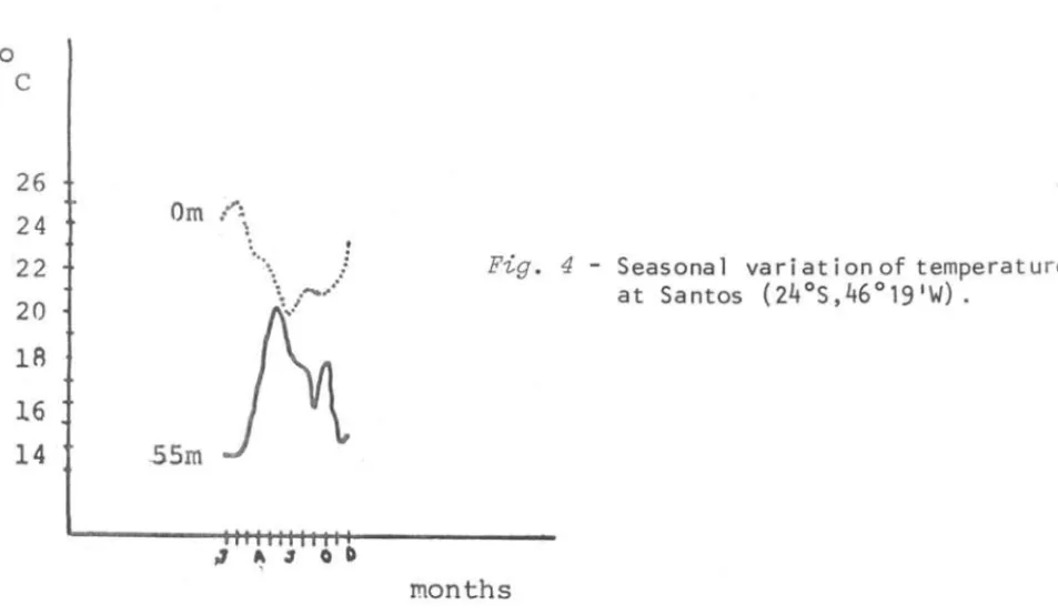
For seasona1 studies long time series are norma11y required but as in tida1 studies the information is basica11y ana1ysed for a known frequency (corresponding to the period of one year) and its theoretica1 spectrum wou1d consist of a sing1e 1ine. Obvious1y real spectrum is contaminated by other features not direct1y seasona1 but often consequences of it.

Figure

4

shows the 12 month1y mean values of temperature taken at

(24°5,

042°W)

for O m and 55 m of depth in coastal waters.

o

C

26 24 22

20

lA

16

14

Om

55m

" A 3 O O

Fig. 4 - Seasona 1 va r i at i on of temperat ure

at Santos (24°S,46°19IW).

rnonths

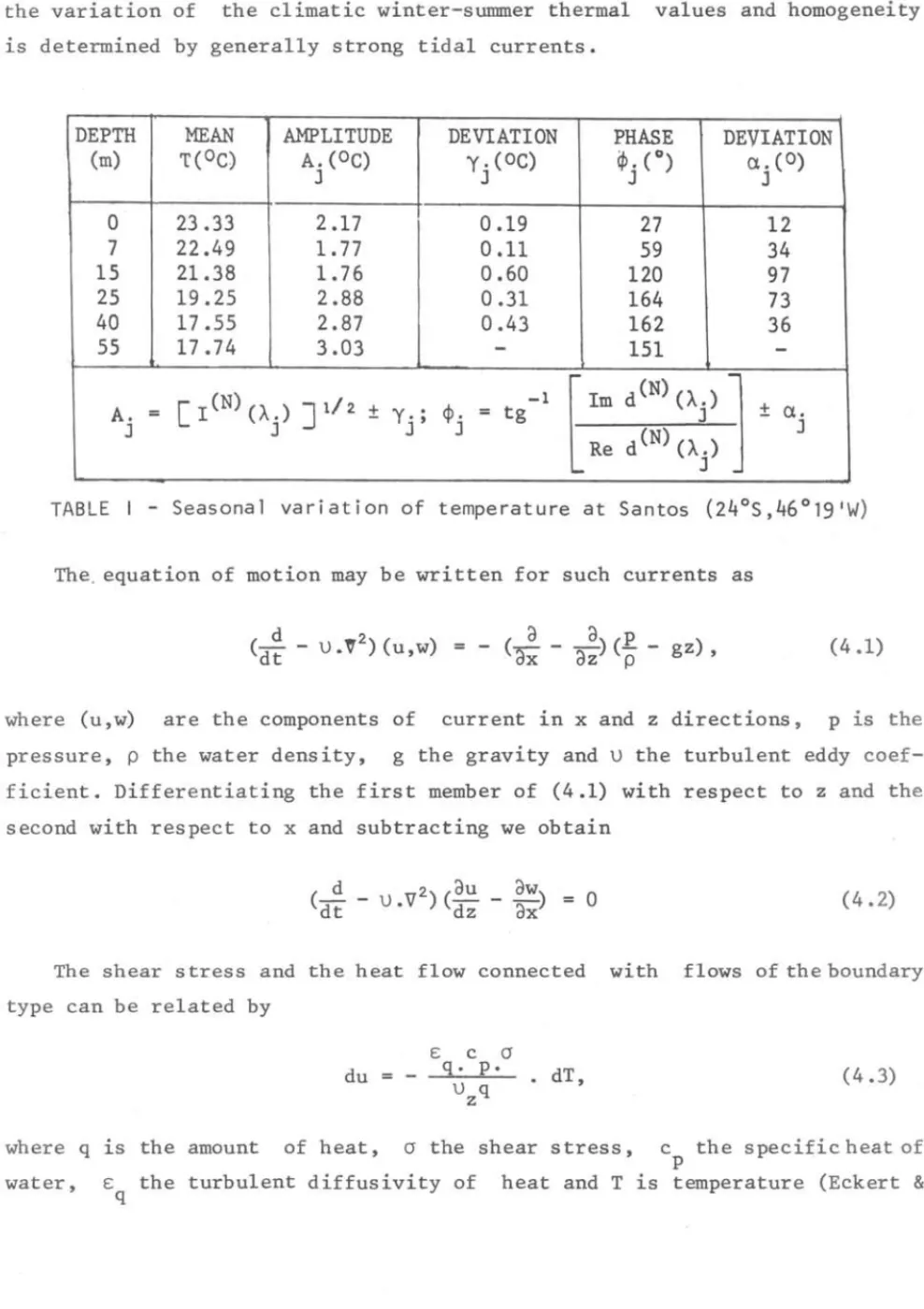
Four years of data were taken for ana1ysis and each year was considered as one rea1ization of the seasona1 processo Deviations ct. where a1so ca1culated

J

from Tab1e I. The 12 mean va1ues of each month, used to ca1cu1ate the ampli-tudes A. according to (2.37), show the main features of Figure 4, namely a

J

seasona1 therma1 inversion between O m and 55 m depths annua1 variation. The other effect (Tab1e I) is that the bottom waters have a greater annua1 amplitude A. of variation than the ones at surface. Amp1itudeis a minimum at

J

15 m with a greater deviation y., indicating the mean annual positioning of

J

the thermoc1ine and that it is a separating 1ine between surface and bottom processes.

MORETTIN

&

MESQUITA:

Spectral methods: oceanography ₁₇₉

those homogeneous values of temperature are in some respect the response to the variation of the climatic winter-summer thermal values and homogeneity is determined by generally strong tidal currents.

DEPTH

MEAN

AMPLITUDE

DE VI ATI ON

PRASE

DEVIATION

(m) T(Oe)

A.

(Oe) y. (Oe)

cp.

(0)

_a.

(O)

J J J J

O

23.33

2.17

0.19

27

12

7

22.49

1.

77

0.11

59

34

15

21.38

1.

76

0.60

120

97

25

19.25

2.88

0.31

164

73

40

17.55

2.87

0.43

162

36

55

17.74

3.03

-

151

-[I(N)

P'j) ] 1/2.

±

-1

t

Im d(N) (Àj )

j

±

A.

= y.; <1>. = tg

a.

J J J

Red(N)(À.)

J

J

TABLE I -

Seasonal variation of temperature at Santos (24°S,46°19I

W)

The, equation of motion may be written for such currents as

d 2.

(dt -

U.' )

(u,w)

=

(ãX -d dZ) d

(p -

p gz),

(4.1)

where (u,w) are the components of current in x and z directions, p is the pressure, p the water density, g the gravity and U the turbulent eddy coef-ficient. Differentiating the first member of

(4.1)

with respect to z and the second with respect to x and subtracting we obtain

(-..i _

U.V2.)(dU _ dW) = O

dt dz

dX

(4.2)

The shear s tress and the heat flow connected with flows of the boundary type can be related by

du

=

. dT,

(4.3)

where q is the amount of heat, cr the shear stress, c the specificheatof p

water, E the turbulent diffusivity of heat and T is temperature (Eckert

&

180 Bolm Inst. oceanogr., S Paulo, 27(2), 1978

Drake, 1959). Similar expression can be written for dw and dTo It follows from (4.2) and (4.3), after neglecting the advective terms, the contribution in the x direction that:

(4.4)

where K is the constant appearing in (4.3) for the z direction. One solution of (4.4) is the diffusion equation, which when solved for T= T.cos(Àt) can be expressed in terms of Fourier components in the form

T(z, t) = TO + _2E 00 A.e -a.z .cos(À.t - az),

j=l J, .1 (4.5)

1/2 where a.

=

(À./2u )

J z h

. 1 "\ 2rr .

and V_z t e vert~ca component of V. For AI

=

12'

AI ~s

the amplitude of the annual component and the first-order term of (4.5) is an exponentially damped wave with increasing depht z, and a corresponding retarding of the phase angle.

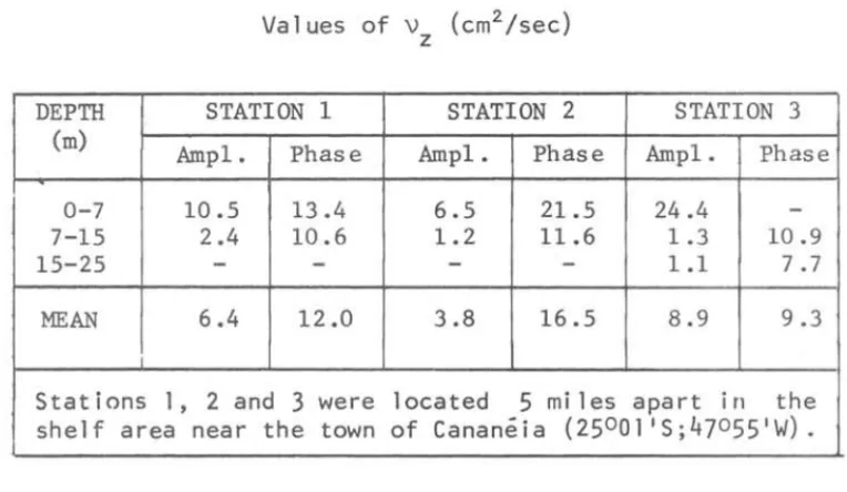
Table 11 shows the results of applying the first term of (4.5) to 12-monthly averaged values of temperature resulting from a four-years of data collection at the shelf area of Cananeia (Lat. 2502'S, Long. 048°W).

DEPTH (m)

0-7 7-15 15-25

MEAN

Stations

Values of V (cm2_/sec)

z

STATION 1 STATION 2 Ampl. Phase Ampl. Phase

10.5 13 .4 6.5 21.5 2.4 10.6 1.2 11.6

-

-

-

-6.4 12.0 3.8 16.5

STATION 3 Ampl. Phase

24.4

-1.3 10.9 1.1 7.7 8.9 9.3

1 , 2 and

3

were located 5 mi les apart i ri the

shelf area near the town of Cananéia (2500l ' S;47055IW) .

MORETTIN & MESQUITA: Spectral methods: oceanography 181

Va1ues of u _z were determined from the damping of AI (amplitude) and the

ret~rding of the annua1 seasona1 cyc1e (Mesquita & Morettin, 1976), are

simi-lar to those of Crawford (1977) determined for the equatorial waters.

5. EQUATORIAL OSCILLATIONS

Meanders of the equatorial waters have recent1y been reported by Düing

et al.,

1975. They have 2,600 km wave 1enght and propagate to the west with a phase speed of 1.9 m/sec. Periodic variation of the fie1d of mass has a1so been found to fo11ow the patterns of a seasona1 variation (Katz

et al.,

1977).

Temperature and sa1inity va1ues of these waters were extensive1y obtained during GATE (GARP At1antic Tropical Experiment) from Ju1y to September, 1974, which showed to be important for the detection of the basic oscillations of the equatorial waters.

Osci11ations are be1ieved to be due to atmospheric forcing (Phi1ander, 1976) and they may occur in the meridional or 1atitudina1 sense.

Determination of the main modes of vibration of the water masses are the basic aim of spectra1 ana1ysis in this case, as no complete theoretica1 hints are yet avai1able.

Therma1 variabi1ity for the entire observationa1 period of GATE (June-September 1974) is shown in Figure 5, for the geographical points (00°, 03So_W),

(02°N, 03SoW) and (02°N,035°W) (Mesquita

et

al., 1977a).

Four 1ayers of distinct thermal variabi1ity can be observed: 1ayer 1 (0-30 m) associated with currents flowing approximate1y East to West; 1ayer

rd

182

O' 10

I.

n'

'0'

lO'

..

~---

---OI

10'

..

O' 10

TEMPERATVAE ·C

.... T[ · ... I

... [ Ilt-.M.'f1tll14

lO

===============-== ,::.

LAr : DIoN

LQHQ' on· ..

TEW'ERA~E ·C

.... f [ oP<c,tlll

K"'tt_H"'Ot·rt/'.

Bolm I nst. oceanogr., S Paulo, 27(2), 1978

••

OI

lO'

..

Fig.

5

-O.

...

LAr: OZ·N

LONO: 038· W

nUPERATUA( ·C

OAT( · (ItIoM 1I ... UII-AUOUITII?,'4

Temperature ti me obta i ned in the phases of GATE.

seri es three

Series of the 4th layer were analysed using estimators of type (2.42),

a-MORETTIN & MESQUITA: Spectral methods: oceanography 183

nalysis, but reasonable estimates of the periodicities were obtained as shown in Figure 6. A special program was used and the numbers of lags for co-variance estimates are indicated in each spectrum. See discussion on the maximum entropy method concerning the availability of few observations .

8.0

N I

o

.-< N

-

u 7.2

_Fig.

₆

-

_{Temperature s pect ra at}

0_ o _,

1,OOOm, during the phase

.

,

II of GATE. 12, 16 and 18

are the numbers of lags 6 . 4

for covari ance est i mates.

,

5.6 ,

I:

,

:

I:

4 . 8 I'

I

I 18

I 16

I

-4.0

I

---

12

I

I

3.2 I

I I

2.4

1.6

0.8

o 0.1 0.2 0.3 0.4 0.5 0.6 0.7 0.8 0 .9 1.0

184

Bolm Inst. oceanogr., S Paulo, 27(2), 1978

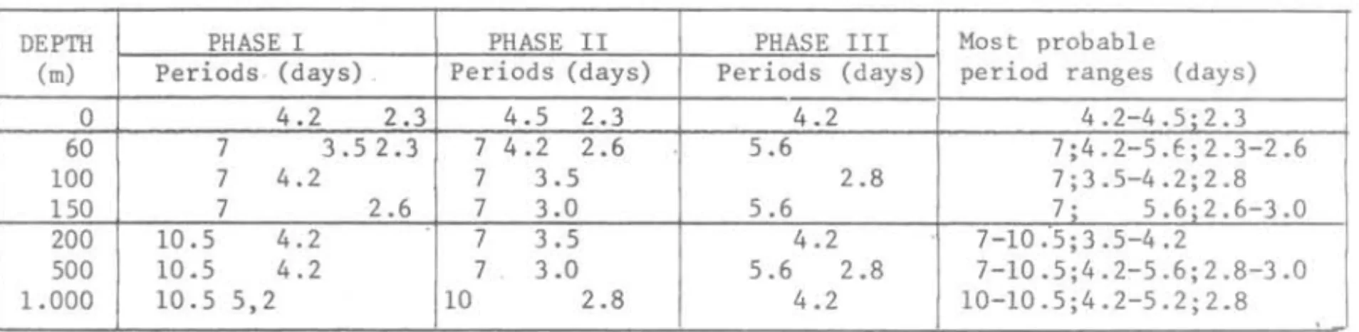
Tab1e 111 shows the most predominant periods in the series of Figure 5, ana1ysed with (2.35), from what we can see the great range of variabi1ity that the equatorial waters undergo. Causes of these variations a1though be-1ieved to be due to atmospheric forcing are sti11 to be proved.

DEPTH

(m)

O

60 100 150 200 500 1.000

TABLE I I I - Periods of the thermal fluctuations of

th~

equatorial area shown in figure

5

PHASE I PHASE II PHASE III Most probab1e Periods · ( days) Periods (days) Periods (days) period ranges (days)

4.2 2.3 4.5 2.3 4.2 4.2-4.5·2.3 7 3.52.3 7 4.2 2.6 5.6 7;4.2-5.E;2 .3-2.6 7 4.2 7 3.5 2.8 7;3.5-4.2;2 .8

7 2.6 7 3.0 5.6 7 ; 5.6;2.6-3.0

10.5 4.2 7 3.5 4.2 7-10 :5;3 .5-4.2

10.5 4.2 7 3.0 5.6 2.8 7-10.5;4.2-5.6;2.8-3.0 10.5 5,2 10 2.8 4.2 10-10.5;4.2-5.2;2.8

The low frequenciesof the spectra were not taken intoaccount, a~thoughbyvisual inspection

they appear to be existent. Periods in each line are distributed in a decreasing arder of magnitude and separated to show approximately the"different behaviour of the layers 1,2,3 and 4 above refered.

The basic difficu1ty of oceanic samp1ing in time series is the short 1enght of the series produced re1ative to the time sca1es of the processes invo1ved. A method for series with few samp1ing points is summarized in next section. Other methods for vectoria1 series are a1so mentioned.

6.

MAX I

MLM ENTROPY (ME) MEll-IOD

MORETTIN & MESQUITA: Spectral methods: oceanography 185

defined to be the expected variance of the prediction error when an auto-regressive mode1 fitted to the present series of X(t) 1S applied to another

independent realization of X(t) to make a one step prediction. See a1so Akaike, 1969b and 1970.

lt seems that this method 1S appropriate when we have short records and

it has the abi1ity to resolve spectra1 peaks better than the other methods. Barber

&

Taylor, 1977, compare the ME method with the 1east-squares method and the smoothing periodogram procedure. For other references on the app1i-cations of this method to oceanography see Ulrych

&

Bishop, 1975 and Chen

&

Stegen, 1974.

7.

ROTARY COMPONENTS

The rotary components method has been app1ied main1y for ana1ys ing current vector time series. The horizontal velocity vector 1!.(t) can be decomposed into a zona1 componentul(t) and a meridional component U2(t). These are assumed to be continuous, stationary stochastic processes with mean zero. lt is known that the coherence is invariant under the app1ication of a linear fi1ter to each series, but it is not invariant under coordinate rotation. In order to accomp1ish this, we decompose the ve10city vector, for each frequency, into two counter-rotating circular motions, each with its own amplitude and phase. See Mooers, 1975.

lf f (À) and f (À) are the auto-spectra of Ul(t) and U2(t),

re-UIUl U2U2

spectively, then it can be shown that the antic10ckwise spectrum is given by

(5.1)

and the c10ckwise spectrum 1S given by

186

Bolm Inst. oceanogr.,

S

Paulo,

27(2), 1978

q (À) being the quad-spectrum between Ul(t) and uz(t). The total spectrum

UIU2

of kinetic energy is given by

(5.3)

The amplitudes of these rotary spectra are independent of the orientation of the coordinate system where the process is described. For applications see Gonela, 1972. The case of rotary bi-spectra is considered by Yao

et al.,

1975, to analyse the non-Gaussian nature of a vector random processo

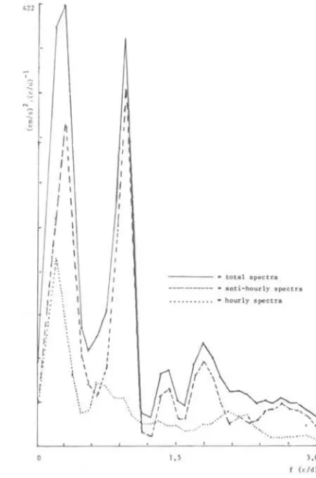
Figure 7 shows the rotary spectra of currents at 25°S045°W. Currents at the area show periodicities of 3-6 days, diurnals and semidiurnals and flow with a pronounced anti-hourly sense (Mesquita

et al.,

1977b).

Fig.

7 - The rotary spectra of currents - 40m.

02' ,-, ] _~ I' "

1' _I

I I I

I

,

I I I ;~

I': C

,:

I: I: t: ,: " j: t 1 r

,

I

,

I I

,

\

,

I

,

\ : \

i \ I

\

\1/"

\ . .J

- - - - total spectra --- • anti-hourly spectra

.•. . .•.... . • hourly spectra

J,5

\

\ ,

\\' " I_'A.. ... _~

.... \-/',.\ / .... ,""'-... ... ~ ... ~~

3,0

f ( c Id)

MORETTIN & MESQUITA: Spectral methods: oceanography 187

B IB LI OGRAPHY

AKAIKE, H. 1969a. Fitting auto-regressive mode1s for prediction. In: Rosenb1att, M. & Van Atta , C., ed. - Statistica1 mode1sand turbu1ence. New York, Springer-Ver1ag .

1969b. Power spectrum estimation through auto-regressive

mode1 fitting. Ann. Inst. statist. Math., Tokyo, 21:407-419.

1970. Statis t ica1 predictor identification. Ann. Inst. statist. Math., Tokyo, 22:203- 217.

BARBER, F. G. & TAYLOR, J. 1977. A note on free oscillations of Chedabucto Bay. Manuscr. Rep. Ser., Mar. Sci. Directorate, Ottawa, (47). BRILLINGER, D. R. 1965. An introduction to po1yspectra. Ann. math.

Statist., 36(5) :1351-1373.

1970. The identification of po1ynomia1 systems by means of higher order spectra. J. Sound Vibr., 12(3):301-313.

1975. Time series - data ana1ysis and theory. New York, Ho1t, Rinehart

&

Winston.

- - - & ROSENBLATT, M. 1967a. Asymptotic theory of esti-mates of K-th order spectra. In: Harris, B., ed. - Spectra1 ana1ysis of time series. New York, Wi1ey

&

Sons, p. 153-188.

1967b. Computation & interpretation

of K-th order spectra. In: Harris, B., ed. - Spectra1 ana1ysis of time series. New York, Wi1ey

&

Sons, p. 189-231.

CARTWRIGHT, D. E. 1971. Some ocean tide measurements of the Eighteenth Century, and their re1evance today. Proc. R. Soc., ser. B, 72(32) :331-339. - - - & EDDEN, A. C. 1973. Corrected tab1es of tida1

harmonics. Geophys. J. R. astro Soc., 33:253-264.

- - - & TAYLER, R. J. 1971. New computations of the tide generating potentia1. Geophys. J. R. astro Soc., 23:45-74.

CHEN, W. Y.

&

STEGEN, G. R. 1974. Experiments with maximum entropy power of sinusoids. J. geophys. Res., 79:3019-3022.

COHEN, A.

&

JONES, R. H. 1969. Regression on a random fie1d. J. Am.

statist. Ass., 64:1172-1182. CRAWFORD, W. R. 1976.

Equatorial undercurrent. Oceanographic Institute.

188 Bolm Inst. oceanogr., S Paulo, 27(2), 1978

DOODSON, A. T. 1921. The harmonic deve10pment of the tide generating

potentia1. Proc. R. Soe., ser. A, 100:305-328.

1957. The ana1ysis and prediction of tides 1n sha110w

waters. Int. hydrogr. Rev., 33:85-126.

DUING, W.; HIZARD, P.; KATZ, E.; MEINCKE, J.; MILLER, L.; MOROSHKIN, K. V.;

PHlLANDER, G.; RYBNIKOV, A. A.; VOIGT, K.

&

WEISBERG, R. 1975.

Meanders and longwaves in the Equatorial At1antic. Nature, Lond.; 257(5524) •

ECKERT, E. R.

&

DRAKE, R. M. 1959. Heat and mass transfere New York,

MacGraw-Hill.

FRANCO, A. dos S. 1964. Harmonic ana1ysis of tides for 7 days of

hour1y observations. Int. hydrogr. Rev., 41(2) :109-142.

- - - & ROCK, N. J. 1971. The fast Fourier transform and its app1ications to tida1 osci11ations. Bo1m Inst. oceanogr., S Paulo,

20: 145-199.

GASSER, T. 1972.

functions. Dissertation Techno1ogy.

System identification, po1yspectra and re1ated (Doctor of Math.). Swiss Federal Institute of

GERSH, W. 1970. Spectra1 ana1ysis of EEG's by auto-regressiv~

decom-position of time series. Math. Biosc., 7:205-222.

GODFREY, M. D. 1965. An exp1oratory study of the bispectrum of

eco-nomic time series. App1. Statist., 14(1):48-69.

GODIN, G. 1972. _{The ana1ysis of tides. Liverpoo1, Liverpoo1 University}

Press, 264p.

GONELLA, J. 1972. A rotary-component method for ana1ysing

meteoro-logica1 and oceanographic vector time series. Deep Sea Res., 19:833-846.

HANNAN, E. J. 1966. Spectra1 ana1ysis for geophysica1 data. J. R.

astro Soe., 11:225-236.

HORN, W. 1960. Some recent approaches to tida1 prob1ems. Int. hydrogr.

Rev., 37(2):65-68.

JENKINS, G. M. & WATTS, D. G.

535p. 1968. Spectral ana1ysis. Holden-Days,

JONES, R. H. 1963. Stochastic processes on a sphere as app1ied to

meteoro1ogica1 500-mi1ibar forecasts. In: Rosenb1att, M., ed. - SIAM

Proc. of Time Series Ana1ysis. New York, John Wi1ey, p. 119-124.

KATZ, E.; BELEVITSCH, R.; BRUCE, J.; BUBNOV, V.; COCHRANE, J.; DUING, W.;

HIZARD, P.; LASS, H. V.; MESQUITA, A. R. de; MILLER, L. & RYBNIKOV, A. A.

1977. Zona1 pressure gradient along the Equatorial Atlantic. J. mar.

MORETTIN & MESQUITA: Spectral methods: oceanography 189

KOOPMANS, L. H. 1974. The spectra1 ana1ysis of time series. New York, Academic Press.

MESQUITA, A. R. de; MAGLIOCCA, A. & ,;illBROSIO Jr., O,. 1977~. Physica1 and chemica1 variability at 35-40'W of the Equator1a1 At1ant~ . c upper 1ayers.

ReI. int. Inst. oceanogr., Univ . S Paulo, (8):1-27.

--- &

MORETTIN, P. A. 1976.

espectral

ã

oceanografia" (in Portuguese) .

and Statistics~ (in press).

"Aplicações da análise

2w ~ Bruzi lian Syrrrp. on Prob.

- - -- - - ; SOUZA, J. M. C. de; TUPINAMBÁ, P. M.; WEBER, R.; FESTA, M.

&

LEITE, J. B. A. 1977b. Correntes rotatórias e

varia-b i lidade do campo de massa na plataforma do Estado de são Paulo (Ponto: 25 S; 46 W). ReI. Cruzeiros, sêr. N/Oc. "Prof. W. Besnard", Inst. oceanogr. Univ. S Paulo, (3):1-27.

MEUS, J. 1962. _{Tab1es of moon and sun. Be1gium, Kess1eberg St.errenwacht.}

MOEERS, C. N. pairs of po1arized 1141.

K. 1973. A technique for the cross spectrum ana1ysis of comp1ex-va1ued time series, with emphasis on properties of components and rotationa1 invariants. Deep Sea Res.,

20:1129-MUNK, W.

&

CARTWRIGHT, D. E. _{1966. Tida1 spectroscopy and predict ion.} Phi1. Trans. R. Soc., ser. A, 259:533-581.

& HASSE~N, K. 1964. Super-reso1ution of tides. In: Yoshida, K., ed. - Stud1es on oceanography. Tokyo, University of Tokyo Press p

339-344. ' •

PARZEN, E. 1972. Some recent advances in the time series ana1ysis . In: Rosenb1att, M.

&

Van Atta, C., ed. - Statistica1 mode1s and turbu1ence. New York, Springer-Ver1ag.

PHILANDER, G. 1976. Instabi1ities of zona1 equatorial currents . J. geophys. Res., 81(21):3725-3735.

ROY, R. 1976. - Spectra1 ana1ysis for a random process on the sphere. Ann. Inst. statist. Math., Toky:o, 28(1):91-99.

190 Bolm Inst. oceanogr., S Paulo, 27(2), 1978

ULRYCH, T. J.

&

BISHOP, T. N. 1975. Maximum entropy spectra1 ana1ysis and auto-regressive decomposition. Rev. geophys. space Phys., 13:183-200. YAO, N.-C.; NESHYBA, S.

&

CREW, H. 1975. Rotary cross-bispectra and energy transfer functions between non-gaussian vector processes.I. De-ve10pment and examp1e. J. phys. Oceanogr., 5(1):164-172.

YAGLOW, A. M. 1961. Second-order homogeneous random fie1ds. Proc. Berkekey Symp. math. Statist. Probab., 4th , 2:593-622.