A Life-cycle Equipment Labeling System for Machine Classification in Smart Factories

A Life-cycle Equipment Labeling System for Machine Classification in Smart Factories

Susana Aguiar, Rui Pinto, Jo˜ao Reis, Gil Gonc¸alves

Faculty of Engineering of University of Porto Rua Dr. Roberto Frias, s/n 4200-465, Porto, Portugal Email: {saguiar, rpinto, jpcreis, gil}@fe.up.pt

Abstract—Nowadays, due to ever decreasing product life cycles and high external pressure to cut costs, the ramp-up of production lines must be significantly shortened and simplified. This is only possible if a forecast of the impact of modification within an existing production environment is available, helping during decision making of production methods. This type of predictions will have a direct impact on the cost-effective production process, maintaining concerns regarding the environmental and social impacts. These are the ideas behind the project Innovative Reuse of modular knowledge Based devices and technologies for Old, Renewed and New factories (ReBorn). The present paper describes the System Assessment Tool, a software application developed in ReBorn, which is used for assessing the sustain-ability of highly adaptive production systems through the use of Reliability, Life Cycle Cost and Life Cycle Assessment metrics, in the form of a equipment labeling scheme. This labeling scheme consists on classifying the dependability of industrial equipment, based on the collected metrics. To that intent, several simulation processes were performed, in order to assess the suitability of the labeling system, in comparison to the Quality metric that is highly preferable among the industrial partners. The simulation results show that a two-layer equipment labeling system is the most suitable approach to be used for classification.

Keywords–Smart factories; Equipment label; Life-cycle assess-ment; Re-use; Production systems.

I. INTRODUCTION

ReBorn was a European Project funded by the Seventh Framework Programme of the European Commission. The vi-sion of ReBorn was to demonstrate strategies and technologies that support a new paradigm for the re-use of production equipment in factories. This re-use will give new life to decommissioned production systems and equipment, helping them to be “reborn” in new production lines. Such new strategies will contribute to sustainable, resource-friendly and green manufacturing and, at the same time, deliver economic and competitive advantages for the manufacturing sector.

The developments made in ReBorn allow production equip-ment to extend its life cycle, contributing to economic and environmental sustainability of production systems [1]. This concept of modular production equipment may also be re-used between different production systems, after servicing and upgrading. This new business paradigm will move from an equipment-based business to a value added business, where equipment servicing and equipment knowledge are main busi-ness drivers.

The proposed paradigm is built on self-aware and knowledge-based equipment, which requires capabilities to collect and manage information, regarding its functionalities,

evolution over time due to its use and wear, and maintenance operations, upgrade and refurbishment over lifetime. For this to be possible, versatile and modular task-driven plug&produce devices, with built-in capabilities for self-assessment and op-timal re-use were implemented, along with strategies for their re-use and models for factory layout design and adaptive configuration.

The ReBorn [2] developments demonstrated to be suc-cessful for intelligent machine repair, upgrade and re-use of equipment, and (re-)design of factory layouts [3]. Most of these developments were demonstrated within several indus-trial demonstration scenarios at 2016 AUTOMATICA fair (21-24 June) in Munich, Germany [4].

During its life-cycle, industrial equipment goes through three main stages, namely 1) the initial incorporation into the production line, 2) the operation and maintenance/upgrade, and 3) the end-of-use and disassemble. Throughout these stages failures or malfunctions can potentially cause costly machine downtime or even downtime in the entire production system. Downtime of equipment operation is usually avoided based on engineers and shop-floor operators decision making, which are most of the times based on the experience of these individuals. Sometimes the individual’s know-how and gained knowledge by experience is hard to be transferred to other individuals and may be lost [5]. This problem was tackled in ReBorn by developing a software tool named Workbench.

The Workbench is a decision making support tool, which combines simulations with the historical process data gath-ered at equipment level. It provides methods and algorithms for assessing the various potential possibilities of industrial equipment, regarding change, upgrade, reuse, dismantle and disposal. These possibilities are evaluated based on the cor-responding reconfiguration effect on the overall system cost, performance and status throughout the life-cycle(s) of the manufacturing system. The analysis and comparison of indus-trial equipment is achieved using a System Assessment Tool (SAT), which performs Life Cycle Cost (LCC) and Life Cycle Assessment (LCA) analysis, based on reliability metrics.

In order to have a more generic and simple way of comparing industrial equipment, the SAT has a functionality, which main goal is to calculate an equipment Label. This Label measures a dependability factor, as for example the appliances energy consumption label, grades equipments from A to F, being A very dependable and F less dependable. This paper presents three simulations that were defined and executed, in order to test the usability and correctness of the Label. The basic idea behind all the three simulations is to use as much

information as possible, from the information available in the SAT, that is, all the metrics that the SAT can calculate. Each metric has a weight associated to it, which was defined based on a questionnaire that was sent to the industrial partners of the ReBorn project. The equipment Label simulations indicate that using all the metrics available in a straight way might not give the best results, because this allows the possibility of having equipments with a Label grade that is higher or lower, with a difference of two or more grades, than the quality grade, which is, for the industrial ReBorn partners, the most important metric. This lead to a two layer Label scheme that provides grading results closer to the values of the most important metrics.

This paper is organized in five more sections. Section II defines the concepts of LCC and LCA and overviews the current state of the art, regarding tools and metrics used to perform this type of equipment analysis. In section III, an overview of the Workbench tool is presented, along with a description of its different modules, including the SAT. In Section IV, a detailed analysis and description of the SAT is presented. Section V explains one of the SAT functionalities, the equipment Label, where several simulations are defined and its results presented and discussed. Finally, Section VI concludes the paper by exposing some final remarks about the work developed.

II. RELATEDWORK

Several models, tools, and standards have been developed to analyze equipment reliability [6], [7], LCC [8]–[12], and LCA [13]–[18]. Although these techniques have usually been treated as separate analysis tools, defined by their own metrics and standards, some authors attempted to bring them closer [19]–[22] by presenting the relation between different sustain-ability assessment tools, focusing on the life cycle assessment as central concept for sustainability [23]. For the interested reader, several surveys of existing methodologies and tools regarding equipment analysis have been performed over the years [11], [21], [23]–[25].

A. Life Cycle Assessment

LCA is an approach for assessing industrial systems from creation to disposal [26]–[30]. This approach begins with the gathering of raw materials of the mother nature to create the product, ending when the product is dismantle and the disposal of all materials to the environment [14], [15].

According to Currant [13], LCA had its beginnings in the 1960’s due to concerns over the limitations of raw materials and energy resources. The work published by Harold Smith [31] is considered as one of the firsts in this field. In that work he reported his calculations of cumulative energy requirements for the production of chemical intermediates and products.

In 1969, researchers initiated an internal study for The Coca-Cola Company (that was not officially published but it is mentioned in most of the LCA works [13], [32], [33]), which laid the foundation for the current methods of life cycle inventory analysis in the United States. In this study, the used raw materials and fuels, as well as the environmental loadings from the manufacturing processes for each container, were quantified. The comparison between the different beverage containers allowed to determine which container had the lowest releases to the environment and which least affected the supply

of natural resources. The process of quantifying the resource use and environmental releases of products became known as a Resource and Environmental Profile Analysis (REPA) in the United States, and as Ecobalance in Europe.

From 1975 through the early 1980’s, as influence of the oil crisis faded, environmental concerns shifted to issues of hazardous and household waste management. However, throughout this time, life cycle inventory analysis continued to be conducted and the methodology improved through a slow stream of about two studies per year, most of which focused on energy requirements. During this time, European interest grew with the establishment of an Environment Directorate (DG X1) by the European Commission [34]. European LCA prac-titioners developed approaches parallel to those being used in the USA. Besides working to standardize pollution regulations throughout Europe, DG X1 issued the Liquid Food Container Directive in 1985, which charged member companies with monitoring the energy and raw materials consumption and solid waste generation of liquid food containers. When solid waste became a worldwide issue in 1988, LCA emerged again as a tool for environmental problems analysis.

In 1991, concerns over the inappropriate use of LCA to make broad marketing claims made by product manufacturers resulted in a statement issued by eleven State Attorneys General in the USA, denouncing the use of LCA results to promote products. Such assessments should be conducted by uniform methods, by reaching a consensus on how this type of environmental comparison can be advertised non-deceptively. This action, along with pressure from other environmental organizations to standardize LCA methodology, led to the de-velopment of the LCA standards in the International Standards Organization (ISO) 14000 series (1997 through 2002) [35].

In 2002, the United Nations Environment Program (UNEP) joined forces with the Society of Environmental Toxicology and Chemistry (SETAC) to launch the Life Cycle Initiative, an international partnership. This Initiative has characterized by three programs: (1) the Life Cycle Management (LCM) pro-gram creates awareness and improves skills of decision-makers by producing information materials, establishing forums for sharing best practice, and carrying out training programs in all parts of the world; (2) the Life Cycle Inventory (LCI) program improves global access to transparent, high quality life cycle data, by hosting and facilitating expert groups work results in web-based information systems; (3) the Life Cycle Impact Assessment (LCIA) program increases the quality and global reach of life cycle indicators, by promoting the exchange of views among experts, whose work results in a set of widely accepted recommendations.

LCA evaluates all stages of a product’s life cycle, from the perspective that they are interdependent, meaning that one operation leads to the next. Figure 1 presents the possible life cycle stages that can be considered in a LCA as well as the typical inputs and outputs measured. LCA enables the estimation of cumulative environmental impacts that resulted from all stages in the product life cycle, often including impacts not considered in more traditional analyses (e.g., raw material extraction, material transportation, ultimate product disposal, etc.). By including these impacts throughout the product life cycle, LCA provides a comprehensive view of the environmental aspects of the product or process and a more accurate picture of the true environmental trade-offs in product and process selection.

The LCA process is a systematic, phased approach and consists of four components as illustrated in Figure 2: 1) Goal Definition and Scope - Define and describe the product, process or activity, by establishing the context in which the assessment is to be made and identify the boundaries and environmental effects to be reviewed for the assessment; 2) Inventory Analysis - Identify and quantify energy, water and materials usage and environmental releases, such as air emis-sions, solid waste disposal and waste water discharges; 3) Im-pact Assessment - Assess the potential human and ecological effects of energy, water, material usage and the environmental releases identified in the inventory analysis. Inputs and outputs are categorized in different impact categories midpoints, such as climate change and land use, and endpoints, such as human health and resource depletion; 4) Interpretation - Evaluate the results of the inventory analysis and impact assessment, in order to select the preferred product, process or service with a clear understanding of the uncertainty and the assumptions used to generate the results.

Figure 2. Phases of a LCA Process.

Conducting a LCA study have the main benefit of develop-ing a systematic evaluation of the environmental consequences associated with the creation of a given product. This evalua-tion provides means to analyze the environmental trade-offs associated with one or more specific products/processes, in order to help the stakeholder gain acceptance for the planned action. Moreover, the evaluation allows to quantify environ-mental releases to air, water and land, in relation to each life cycle stage and/or major contributing process, assisting in the identification of significant shifts in environmental impacts between life cycle stages and environmental media. Also, the assessment of the human and ecological effects of material consumption and environmental releases to the

local community, region, and world allows to identify impacts to one or more specific environmental areas of concern and compare the health and ecological impacts between specific products/processes.

However, LCA studies may present some limitations, such as very high resource and time consuming processes. Data gathering can be problematic, due to availability issues, result-ing in inaccuracy of the final results. Also, a LCA study will not determine which product or process is the most cost ef-fective or works the best. The information provided by a LCA study is used as a small component of a more comprehensive decision process, such as Life Cycle Managements.

B. LCC - Life Cycle Costing

LCC is a process used to determine the sum of all the costs associated with an asset or with part of an asset. These costs include acquisition, installation, operation, maintenance, refurbishment, and disposal. LCC can be carried out during any or all phases of an asset’s life cycle. LCC processes usually include steps such as [8], [10]–[12], [19]: 1) Life Cost Planning, which concerns the assessment and comparison of options/alternatives during the design/ acquisition phase; 2) Selection and development of the LCC model, namely designing cost breakdown structure, identifying data sources and uncertainties; 3) Application of LCC model; and 4) Documentation and review of LCC results.

The main goal for carrying out LCC calculations is to aid decision making regarding assessment and control of costs, by identifying cost significant items, selection of work and expenditure of planning profiles. Early identification of acquisition and ownership costs enables the decision-maker to balance performance, reliability, maintenance support and other goals against life cycle costs. Decisions made early in an asset’s life cycle have a greater influence on the Life Cycle Costing than those made late, leading to the development of the concept of discounted costs. The LCC process can be divided into several steps, which are represented in Figure 3. As it can be seen in this figure, the LCC process has 6 stages, that are divided into two groups. The first step is to develop a plan that addresses the purpose, and scope of the analysis. The second step is the selection or development of the LCC model that will conform with the objectives of the analysis. Step three is the application of the model defined in step two. In Step four all the results gathered in the analysis are documented, and the Life Cost Planning phase is finished. In Step five, the model defined in step two is applied using nominal costs, initiating the Life Cost Analysis. Finally, step six involves the continuous monitoring in order to identify areas in which cost savings may be made and to provide feedback for future life cost planning activities. This step finishes the Life Cost Analysis phase. All these steps may be performed iteratively as needed. Assumptions made at each step should be rigorously documented to facilitate iterations and to help in the interpretation of the results of the analysis. The method used to estimate the cost elements in LCC calculations will depend on the amount of information needed to establish the usage patterns and operational characteristics, in order to infer the expected remaining life, along with the information needed to understand the technology employed. In [12] several methods are presented. The Engineering Cost Method is used when there is detailed and accurate capital and

Figure 3. LCC Process.

operational cost data for the study. It involves the direct esti-mation of a particular cost element by examining component-by-component. It uses standard established cost factors, such as firm engineering and/or manufacturing estimates, in order to develop the cost of each element and its relationship to other elements (known as Cost Element Relationships - CER). The Analogous Cost Method provides the same level of detail as the Engineering Cost Method, but draws on historical data from similar components that have analogous size, technol-ogy, use patterns and operational characteristics. Finally, the Parametric Cost Method is employed when actual or historical detailed component data is limited to known parameters. These available data from existing cost analyses is used to develop a mathematical regression or progression formula, which can be solved for the cost estimate required.

The basic deterministic methods are underlying virtually all LCC investigations. The process begins with the customer needs and ultimately ends with the customer selecting a preferred option. In this context, the LCC procedure em-ployed is used to support a decision-making process focused on customer satisfaction. The deterministic approach assigns each LCC input variable a fixed discrete value. The analyst determines the most likely input parameters values that occur, usually based on historical evidence or professional judgment. Collectively, these input values are used to compute a sin-gle LCC estimation. Traditionally, applications of LCC have been deterministic ones. A deterministic LCC computation is straightforward and can be conducted manually using a calculator or automatically with a spreadsheet. However, it fails to convey the degree of uncertainty associated with the Present Value (PV) estimate.

The deterministic method of the LCC investigations allows to have a logical ordering of analytical activities and a means of ranking [11]. This ranking includes feasible options for the construction, refurbishment, and on-going management and support of infrastructures. However, this straightforward deterministic approach provides little guidance to the engineer or designer, which attempts to adequately represent the com-plexity and uncertainty inherent to LCC investigations. For this reason, the basic method is usually extended. A common extension to the basic method of LCC involves the use of sensitivity analysis and risk analysis [37]. Sensitivity analysis involves the behavior of model variables over predetermined bounds to determine their relative effect on model outcome. Through this process, analysts can identify some subset of model variables that exert significant influence on model re-sults and/or determine break-even points that alter the ranking of considered options.

Following an initial deterministic ranking of feasible design options, sensitivity analysis is employed to establish the

sen-sitivity of model results and rankings across model variables of particular concern to analysts and decision makers. While sensitivity analysis provides decision-makers insights regard-ing the flexibility of model results across a range of variable estimates and corresponding bounds, it has some shortcomings. First, it may fail to identify a dominant alternative among considered design options. This is certainly the case where perturbations in model variables disturb the ranking of feasible design options. Second, since sensitivity analysis typically involves the independent perturbation of each model variable, engineers and, therefore, customers do not gain a sense of the combined and simultaneous influence of several “perturbed” model variables on LCC results and rankings. Finally, in the absence of defined probability distributions, the likelihood that particular values occur is unexplored.

The purpose of risk analysis is to address these shortcom-ings through probabilistic comparison of considered options. Used properly, risk analysis addresses the bulk of limitations associated with sensitivity analysis.

C. Tools

Currently, there are several tools that can perform LCA and/or LCC calculations. In this subsection, some of the most commonly used tool will be briefly described.

The Economic Input-Output Life Cycle Assessment (EIO-LCA) [38] method estimates the materials and energy re-sources required for activities in the economy, and the environ-mental emissions resulting from those activities. Researchers at the Green Design Institute of Carnegie Mellon University operationalized the Leontief’s method in the mid-1990s, since sufficient computing power was widely available to perform the large-scale matrix manipulations required in real-time. Their work consisted on developing a user-friendly on-line tool that implemented the EIO-LCA method. The website performed fast and easy evaluations to a commodity or service, as well as its supply chain. The EIO-LCA method, models, and results represent the inventory stage of the LCA. The results are used to estimate the environmental emissions or resource consumption associated with the life cycle of an industrial sector. However, it fails to estimate the actual environmental or human health impacts that the emissions or consumption patterns cause. The results of the EIO-LCA analysis represent the impacts from a change in demand on an industrial sector. As a LCA tool, the EIO-LCA models applied are incomplete, since the included environmental effects are limited.

EconomyMap [39] is another tool, which uses CEDA 3.0 LCA Economic Input/Output (EIO) database [40], to provide visualization of the same economic activity and indirect en-vironmental impacts. It provides an easy way to dynamically explore and understand the sources and flow of goods, services, and environmental impacts among major industrial sectors. EconomyMap is intended to be a free resource for public interest lawyers and policymakers, to help them identify and prioritize opportunities to reduce environmental impacts. It also serves as an educational resource for broader audiences.

openLCA [41] is a professional LCA tool and footprint software created by GreenDelta in 2006, with a broad range of features and many available databases. It is an open source software and is publicly available to be modified, offering resources such as professional life cycle modeling, up-to-date

usability, a broad choice of life cycle databases and a collab-oration environment for teams. Gabi6 [42] is a sustainability solution with a powerful LCA engine to support several appli-cations, namely Life Cycle Assessment, Life Cycle Costing, Life Cycle Reporting and Life Cycle Working Environment.

Gabi6 - GaBi [42] is a product sustainability solution with a powerful LCA engine to support the following applications: (1) LCA, characterized by the design for environment, eco-efficiency, eco-design and efficient value chains. Products should meet environmental regulations, by reducing material, energy and resource use, as well as smaller environmental footprints such as fewer GHG emissions, reduced water con-sumption and waste. Also, the efficiency of value chains should be enhanced; (2) LCC, characterized by the designing and optimization of products and processes for cost reduction; (3) Life Cycle Reporting, characterized by the product sustain-able marketing, sustainability reporting and LCA knowledge sharing. Environmental communication, product sustainability and analysis for internal departments, management and supply chain should be reported, using product sustainability claims and Environmental Product Declarations (EPDs); (4) Life Cycle Working Environment, characterized by a responsible manufacturing, where manufacturing process should address social responsibilities.

III. WORKBENCH

The Workbench is a web based on-line tool developed in the scope of the ReBorn project, used to demonstrate novel factory layout design techniques. This tool will help manufacturers to keep their production at an optimal level of efficiency and, therefore, at the most optimal point of operation in terms of time, costs and quality. The Workbench integrates five different models to support the system design phase, namely the Requirements Configurator, the Marketplace, the Solution Generator, the System Assessment Tool, and the Layout Planner. The Workbench user interface is represented in Figure 4.

Figure 4. ReBorn Workbench Web Application.

The Workbench offers a fully integrated environment for generating multiple solutions, aiming at reducing significantly the time of the overall design process. It also provides the ability to explore the different solutions generated by the different tools, which opens the scope for considering options within a reduced time frame. It has the capability to ask and

receive component’s data, needed for a dedicated simulation task. With the help of real data, based on discrete event simulations, the Workbench helps to ensure shorter ramp-up and change-over times and, therefore, reduce costs. The different modules can run independently or they can work together, through the modification and sharing of Automation Markup Language (AML) files [43]. The Workbench modules will be described in the next sections.

A. Requirements Configurator Module

The Requirements Configurator is a tool for gathering all key requirements of a production line and provide the captured data in a formalized way. This process achieved by a web ap-plication, which guides the user through several forms, in order to collect its inputs. Each user is asked to input information regarding the company (name and country), the factory, such as available space and the layout, Key Performance Indicators (KPIs), components that are required for the production (di-mensions and required feeder), and assembly processes, which specifies how an assembly is built together. The requirements information is stored and available to be re-used later, when different scenarios or corrections are considered. As soon as the requirements specifications are stored, they are formalized in the ReBorn enhanced AutomationML format and exported in AML file, which will be used by other modules in the Workbench for further processing. Figure 5 represents the Requirements Configurator web application.

Figure 5. Requirements Configurator Web Application.

B. Marketplace Module

The ReBorn Marketplace (RBM) [44] is an on-line plat-form that allows industrial equipment owners and buyers to have a common ground to communicate, offering services like Platform as a System (PaaS). The RBM enables a multi-sided environment that allows connection between market actors, regarding industrial equipment re-selling. Figure 6 represents the Marketplace web application.

The RBM is a n-sided market, with service providers on one end and service consumers on the other. This market is attractive to service suppliers, since they are able to quickly respond to demand. This demand side is comprised of any potential end-user to the services being provided in the plat-form. Service Consumers comprise the marketplace partici-pants, which mainly relate to the RBM service offerings. The Marketplace Service Suppliers can normally be instantiated by any entity capable of offering its services to the platform

Figure 6. Marketplace Web Application.

while altogether adding value to the platform’s base propo-sition. Service Suppliers are industrial equipment builders who provide equipment, as well as equipment information, functionalities (software), and operations. Entities capable of providing complementing services to the platform, in order to co-create value, are labeled as Complementors. These can be, for instance, independent software developers that provide additional equipment functionalities.

C. Solution Generator Module

The Solution Generator provides configuration solutions, based on the established requirements gathered by the Require-ments Configurator and the existing equipment modules (both old and new). This module requires the use of IBM ILOG CPLEX [45], which is a software optimization package. The Solution Generator uses the information in the AML file to significantly reduce the solution space. Then, it generates an AML file for each of the optimized solutions generated. Figure 7 represents the Solution Generator module.

Figure 7. Solution Generator Application.

D. Layout Planner Module

The Layout Planner is the component of the Workbench responsible for finding the optimized layout for the factory shop floor. It delivers an equipment layout solution, taking into consideration several constraints like space restrictions, equipment to be included and restrictions on material flow. The Layout Planner provides several optimization methods in order to find a solution that minimizes the total cost of material handling associated with the equipment layout considered. This cost is calculated by the the sum of the costs of having specific equipment located in a given area of the shop floor layout and the costs of material handling between equipment. Material handling costs are represented by the relationship between flow of material and distance between equipments. Pinto et al. [3] developed an approach based on Genetic Algorithms (GA), which was implemented in the Layout Planner and proved to be more efficient that other genetic algorithm approaches to tackle Facility Layout Problems (FLP). Figure 8 represents the Layout Planner module.

Figure 8. Layout Planner Web Application.

E. System Assessment Tool Module

The SAT integrates reliability and life cycle status informa-tion during early design and costing of assembly automainforma-tion projects. The life-long cost assessment of the system is accom-plished through the data collection of the system performance throughout its life cycle. Based on this performance data, the SAT performs the life cycle cost assessment and analysis of the effect on the overall reconfigured system. Figure 9 represents the SAT module.

The SAT is able to compare machines and production lines in terms of: 1) Reliability metrics, such as failure rate, Mean Time Between Failure (MTBF), Mean Time To Re-pair (MTTR), reliability, availability, performance, quality and Overall Equipment Effectiveness (OEE); 2) LCC metrics, such as Future Value (FV), PV, Net Present Cost (NPC) and Net Present Value (NPV) with initial costs; and 3) LCA metrics, such as life cycle emissions and impact categories, like Global Warming Potential or Ozone Depleting Potential. A detailed overview of the SAT is presented in the next section.

IV. SYSTEMASSESSMENTTOOL

The SAT has two main objectives, namely providing an easy and intuitive way for a user to compare machines or production lines and providing a web API service, capable of receiving requests and share the results with the other modules

Figure 9. System Assessment Tool Web Application.

in the Workbench or other future applications. As mentioned before, the SAT provides an easy and intuitive way for a user to compare machines or production lines, in terms of reliability, LCC, LCA, classifying each machine with a label, based on a grading system. Figure 10 represents an overall architecture of the SAT, which consists on four main groups of metric parameters: 1) Reliability; 2) LCC; 3) LCA and 4) Equipment Label. These groups will be further detailed in the next sections.

Figure 10. System Assessment Tool Overall Architecture.

Regarding communication interfaces, the SAT can interact directly with the Marketplace, as represented in Figure 11, or it can interact with other applications, using a web API or the available web interface. The SAT is prepared to receive requests for performing analysis of equipment, using the available metrics, where both equipment information and the analysis results are imported/exported to an AML file or stored locally into a database.

Available machines in the Marketplace can be compared with machines available in the SAT scope. The user can select from a list the machines to be compared and perform the analysis. Figure 12 represents and example of the results provided by a comparison analysis between two industrial machines. In this case reliability metrics are shown. Each graph shows the percentage of each equipment for each metric. A. Reliability Metrics Functionality

Regarding reliability metrics of equipment operation, the SAT [1] can calculate several parameters, namely the failure

Figure 11. SAT - Marketplace Connection.

Figure 12. Machine comparison - Reliability metrics.

rate, MTBF, MTTR, reliability, availability, performance, qual-ity and OEE.

1) Failure rate: Failure rate, represented by F r, can be defined as the frequency that an engineered system or compo-nent fails. F r is calculated by the ratio between the number of failures F that occur and the operating time Ot of the

equipment, as shown in Equation (1).

F r = F Ot

2) Mean Time Between Failure: MTBF, represented by M T BF , is defined as the predicted elapsed time between inherent failures of a system during operation. It is the inverse of the Failure Rate and is thus calculated from the same parameters, namely the number of failures F that occur during the operating time Ot, as shown in Equation (2).

M T BF = Ot

F (2)

3) Mean Time To Repair: MTTR, represented by M T T R, is a basic measurement of the maintainability of repairable items, which reflects both the severity of breakdowns and the efficacy of repair activities. It represents the average time required to repair a failed component or device and depends on the number of expected breakdown times Dt and the number

of failures F in a given period of time, as shown in Equation (3). M T T R = N X n=1 Dtn F (3)

4) Reliability: Reliability, represented by R, is the prob-ability that the equipment will finish successfully a task of duration t without failures, as shown in Equation (4).

R = e−(F r×t) (4)

5) Availability: Availability A represents the percentage of scheduled time that the operation is available to operate. It is defined as the ratio between the actual operating time Otand

the scheduled production time of an equipment Pt, as shown

in Equation (5).

A = Ot Pt

(5) The scheduled production time of an equipment Pt can

be calculated as the sum of the operating time Ot with the

expected down time Dt, as shown in Equation (6).

Pt= Ot+ Dt (6)

6) Performance: Performance P represents the speed at which the equipment runs as a percentage of its designed speed. It is the ratio between the actual number of units produced P t and the number of units that theoretically can be produced, considering the rate of operation that the equipment is designed for, represented by the ideal cycle time Ct, as

shown in Equation (7).

P = P t × Ct Ot

(7) 7) Quality: Quality Q represents the good units produced as a percentage of the total units produced. It is the ratio between the number of good units P g and the total number of units P t that were produced, as shown in Equation (8).

Q = P g

P t (8)

8) Overall Equipment Effectiveness: OEE, represented as OEE, quantifies how well a manufacturing unit performs relative to its designed capacity, during the periods when it is scheduled to run, which can be determined by the the ratio between the theoretical maximum good output during the production time and the actual good output. Equation (9) represents a practical form to calculate the OEE, which depends on the availability A, the performance P and the quality Q.

OEE = A × P × Q (9)

B. LCC Metrics Functionality

Regarding LCC metrics, the SAT performs calculations regarding the Capital Cost Unit Over Service Life, the Capital Annualized Cost Unit, the future and present values, Net Present Cost and Net Present Value.

1) Capital Cost Unit Over Service Life: Capital Cost Unit Over Service Life CC represents the cost of producing a unit over the equipment expected service life. As shown in Equation (10), this cost is calculated by the sum of all costs associated with the equipment, namely: 1) acquisition and installation TCi; 2) operation and maintenance TCm, considering also the

energy consumption (where ce is the default annual energy

consumption, re is electricity rate and Esl is the equipment

expected service life); and 3) disposal TCe.

CC = TCi+ TCm+ Esl× (ce× re) + TCe (10)

Acquisitions and installation costs include hardware and software acquisitions, service contracts, administrative, set up installation and other initial costs. Operation and maintenance costs include training maintenance support, material costs, equipment upgrade and other maintenance operation. Oper-ation and maintenance costs include the equipment energy consumption, where the default annual energy consumption ce can be calculated using the power consumption in active

P wa and sleep mode P ws, and the time that the equipment

is turned off Tof f and in standby Tsleep during workdays, as

shown in Equation (11).

ce= 365 × (P wa+ P ws) × 24 × (1 − (Tof f+ Tsleep)) (11)

2) Capital Annualized Cost Unit: Capital Annualized Cost Unit CA is the cost of the equipment producing a unit per year, which depends on the Capital Cost Unit Over Service Life CC and the machine expected service life Esl, as shown

in Equation (12).

CA =CC

Esl

(12) 3) Future Value: FV, represented as F V in Equation (13), is the economical value of an asset at a specified date in the future, which is equivalent to the economical value of a specific sum today. Based on the time value of money, the value of an equipment today is not equal to the value of the same equipment in a future time. In this case, F V grows linearly, since it’s a linear function of the initial investment Ci. Ci is based on the initial acquisitions and installation

costs, such as hardware and software acquisitions, service contracts, administrative, set up installation and other initial costs. F V also depends on the interest rate r and the time for the equipment to be analyzed T .

F V =

N

X

n=1

Cin× (1 + r × T ) (13)

4) Present Value: PV, represented as P V in Equation (14), is the economical value in the current day of an equipment that will be received in a future date. Costs that occur at different points in the equipment life cycle cannot be compared directly because of the varying time value of money. They must be discounted back to their present value through, e.g., Equation (14), where P V depends on the value in the future F V , the interest (discount) rate r and the time (number of years) for the equipment to be analyzed T .

P V = F V

(1 + r)T (14)

5) Net Present Cost: NPC, represented as N P C in Equa-tion (15), is the sum of all costs, such as capital investment, non-fuel operation and maintenance costs, replacement costs, energy costs, such as fuel costs and any other costs, such as legal fees, etc, after taking into account the interest rate. If a number of options are being considered, then the option with the lowest NPC associated will be the most favorable financial option. N P C depends on the present value P V , the discount rate r and the total cash flow TCf over the reviewed period.

N P C = P V + r × TCf (15)

6) Net Present Value: NPV is used to determine the prof-itability of an investment that is calculated by subtracting the present values of cash outflows from the present values of cash inflows over a given period of time. The NPV may consider or not the initial costs, which are represented as the Net Present Value without Initial Costs N P Vwo and Net Present Value

with Initial Costs N P Vwi, shown in Equations (16) and (17)

respectively. They depend on the cash flows Cf during the reviewed period T , the discount rate r and, in the case of N P Vwi, it is considered the initial costs Ci.

N P Vwo= T X t=1 Cft (1 + r)t (16) N P Vwi= T X t=1 Cft (1 + r)t− Ci (17)

C. LCA Metrics Functionality

The LCA is a “cradle-to-grave” approach for assessing industrial systems. The realization of an LCA study is a complex process that needs large amounts of different data, which usually is not commonly available. For that reason, most of the times, only simpler metrics related to the environmental impacts and their characterization are considered, such as global warming, stratospheric ozone depletion and human health.

1) Global Warming: Global Warming Potential, repre-sented as GW P in Equation (18), is calculated over a specific time interval, commonly 20, 100 or 500 years, and is expressed as a factor of carbon dioxide [15]. To calculate this impact, several types of flows must be taken into account, such as Carbon Dioxide CO2, Nitrogen Dioxide N O2, Methane CH4,

Chlorofluorocarbons (CFCs) like Sulfur Hexafluoride SF6,

Hydrochlorofluorocarbons (HCFCs) like Nitrogen trifluoride N F3 and Methyl Bromide CH3Br.

GW P = CO2+ 25 × CH4+ 5 × CH3Br + 298 × N O2

+ 22800 × SF6+ 17200 × N F3

(18) 2) Stratospheric Ozone Depletion: Stratospheric Ozone Depletion, represented as ODP in Equation (19), is characterized by the Ozone Depleting Potential [15]. ODP of a chemical compound is the relative amount of degradation to the ozone layer it can cause. To calculate this impact, several types of flows must be taking into account, such as CFCs, HCFCs and Halons. CFCs include Dichlorodifluoromethane CCl2F ,

Trichlorofluoromethane CCl3F , Trichlorotrifluoroethane

C2Cl3F3, Dichlorotetrafluoroethane C2F4Cl and

Chloropentafluoroethane C2ClF5. HCFCs include

Chlorodifluoromethane CHClF2 and Trichloroethane

CH3CCl3. Halons include Bromotrifluoromethane

CF3Br, Bromochlorodifluoromethane CF2BrCl and Tetrachloromethane CCl4. ODP = CCl2F + CCl3F + 1.07 × C2Cl3F3 + 0.8 × C2F4Cl + 0.5 × C2ClF5 + 0.055 × CHClF2+ 0.12 × CH3CCl3 + 16 × CF3Br + 4 × CF2BrCl + 1.08 × CCl4 (19) 3) Human Health: Human Health, represented as HH in Equation (20), is characterized by the median lethal concen-tration (LC50) and calculates the amount of toxic material released [15]. To calculate this impact, several types of flows must be taking into account, such as Carbon Monoxide CO, Nitrogen Oxide N Ox and Sulfur Dioxide SO2.

HH = 0.012 × CO + 0.78 × N Ox + 1.2 × SO2 (20)

TABLE I. Metrics Weights Used in Simulations 1 and 2. Metric Type Metric Use / Willing (%) Import. WV 1 WV 2 WV 3 Reliability F r 75% 55% 0.05 0.04 0.04 M T BF 100% 91% 0.09 0.09 0.09 M T T R 100% 91% 0.09 0.09 0.09 R 75% 48% 0.04 0.03 0.03 A 100% 90% 0.09 0.09 0.09 P 75% 93% 0.09 0.09 0.09 Q 100% 98% 0.10 0.20 0.23 OEE 100% 80% 0.08 0.07 0.07 LCC CC 100% 83% 0.08 0.07 0.07 CA 75% 45% 0.04 0.03 0.03 N P Vwo 25% 33% 0.03 0.02 0.01 N P Vwi 25% 28% 0.02 0.01 0.01 N P C 50% 43% 0.04 0.03 0.03 F V 25% 18% 0.01 0.01 0.00 P V 25% 18% 0.01 0.01 0.00 LCA Ec 100% 75% 0.08 0.07 0.07 Rm 75% 40% 0.04 0.03 0.03 Ic 50% 34% 0.02 0.02 0.02

Figure 14. Metrics Questionnaire Results Resume.

D. Equipment Label

The equipment Label is a form of equipment classification, based on the results of the metrics calculated in the SAT, described in sections IV-A, IV-B and IV-C. The classification consists on assigning a grade from A to F to the considered equipment, being A very dependable and F less dependable, as represented in Figure 13, similar to the labeling of the European Union energy [46]. Grades are determined by the sum of the analysis metrics (Reliability, LCC, and LCA), after attributing weights to each of the metrics.

Aguiar et al. [1] presented a simple grading system that is represented in 21 to calculate the label L. This first approach used a few of the possible metrics (along with the corre-sponding weights), such as reliability R, Overall Equipment Effectiveness OEE, initial Ci, operational Cm and disposal Ce costs, energy consumption Ec and percentage reusable P r.

L = WR× R + WOEE× OEE +

Cm W × (Ci + Ce) + WEc× Ec + WP r× P r

(21)

V. TESTS ANDRESULTS

Although Aguiar et al. [1] presented good labeling results based on the most commonly used metrics calculated by the SAT, some industrial companies may have different priorities regarding the metrics used for the analysis. For this reason, in order to identify the importance of the metrics used, a survey was carried out among the industrial partners of the ReBorn Consortium. This survey consisted on a questionnaire, where industrial partners specify the metrics that they usually use and the importance of each metric. Figure 14 represents a resume of the results gathered from the survey.

After inspection of the survey results, it is clear that some metrics are more relevant that others. The most important metric is Quality Q, with an importance of 98%, followed by MTTR M T T R, MTBF M T BF and Availability A, which all have an importance above the 90%.

Based on the information that resulted from the survey, a new labeling system was devised, as shown in Equation (22). In this case, Label L depends on several metrics and the cor-responding weights, namely the Failure Rate F r, Mean Time Between Failures M T BF , Mean Time To Repair M T T R, Reliability R, Availability A, Performance P , Quality Q, Overall Equipment Effectiveness OEE, Capital Cost Unit Over Service Life CC, Capital Annualized Cost Unit CA, Net Present Value without Initial Costs N P Vwo, Net Present Value

with Initial Costs N P Vwi, Net Present Cost N P C, Default

Energy Consumption ce, percentage of recyclable material Rm

and the sum of the impact categories values Ic.

L = WF r× F r + WM T BF × M T BF + WM T T R× M T T R + WR× R + WA× A + WP× P + WQ× Q + WOEE× OEE + WCC× CC + WCA× CA + WN P Vwo× N P Vwo+ WN P Vwi× N P Vwi + WN P C× N P C + Wce× ce+ WRm× Rm + WIc× Ic (22) In order to be widely accepted, the labeling system must be simple, clear and generic enough to be used by different industrial users, with different metric priorities. To validate the effectiveness of the labeling system, represented in Equation (22), three different simulations were performed in a Matlab environment and are presented in the next sections.

All three simulations have the same principles. It was assumed that the values for the metrics were normalized and are expressed in percentage. The metrics values were assigned based on a 1000 uniformly distributed random generated numbers. For Simulation 1 and 2 the corresponding metrics weights were generated in three different versions (WV 1, WV 2

andWV 3), which are presented in Table I. WV 1 was defined

based on the importance given by each industrial partner of the ReBorn Consortium. The other weight versions were defined by increasing the Quality value, because it is the metric with higher importance, and decreasing the value of the metrics

with lower importance, keeping in mind that the sum of all weights is equal to 1. For Simulation 3, the same philosophy is applied, in terms of the weight calculation. The difference between Simulation 3 and Simulation 1 and 2, is that the weight calculation for the first layer in Simulation 3 is done in blocks (Reliability, LCC, and LCA).

To be able to compare all the simulations, the mean and standard deviation are calculated for four different values: 1) number of quality values lower than the Label; 2) number of quality values lower than the Label by two or more grades; 3) number of quality values higher than the Label; 4) number of quality values higher than the Label by two or more grades. Ideally, all the four values, as well as it’s mean and standard deviation values, should be as small as possible. Having small values for mean and standard deviation means that the difference between the metrics used (e.g., Quality) and the equipment Label is short, and the influence of such metrics is very high regarding the Label being calculated.

A. Simulations 1 and 2

Regarding the simulations 1 and 2, the simulations consist on calculating the equipment Label, based on the metrics and the corresponding weights, as shown in Equation (22). For Simulation 1, Figure 15 presents the relationship of the Quality values and the equipment Label calculated for the three versions of metrics weights. From the figure and after observing the results, several equipment labels were identified, where the most important metrics refereed previously had values much lower or higher than the equipment label, that is, with a difference of two or more grades between the equipment Label and the most important metrics.

Figure 15. Simulation 1 - Quality values for the three metrics weights versions.

In order to have a meaningful labeling system that is truthfully usable by the industry, the label classification must reflect the most important metrics that are relevant for the users. Based on the survey performed, Simulation 2 consisted on calculating the equipment Label, considering the most im-portant metrics that resulted from the survey, namely Quality, MTBF, MTTR, and Availability.

In Simulation 2, the equipment Label was calculated using Equation (22), the same way as used in Simulation 1. The difference lays in the importance given for specific metrics. For all the equipment Labels that differ from the Quality value, the Label is recalculated using only the top four metrics, as shown in Equation (23).

L = WM T BF × M T BF + WM T T R× M T T R

+ WA× A + WQ× Q

(23)

Figure 16. Simulation 2 - Quality values for the three metrics weights versions.

The results of Simulation 2 are presented in Figure 16, which consists on the relationship of the Quality values and the equipment Label calculated for the three versions of metrics weights.

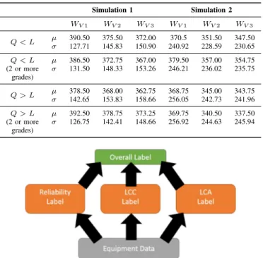
The mean µ and standard deviation σ of the number of equipments that have a Quality value higher or lower then the Label, were calculated and are presented in Table II. This allows for a better understanding and comparison of the simulations results, and to evaluate if the equipment Label calculated is more or less accurate when compared with the Quality value of the equipment. The equipments considered were those who present a Quality different from the calculated equipment Label, and that the difference is higher than one grade from the labeling system.

B. Simulation 3

Taking into account the results from the previous Simula-tions 1 and 2, and based on the fact that the most important metrics chosen from the industrial partners belong to the Reliability metrics group, a different approach was taken in Simulation 3, where the equipment Label calculation is performed at two levels, as represented in Figure 17. First, the equipment Label is calculated three times, one from each metric group, namely Reliability, LCC and LCA metric groups. These Label results will be used to calculate an overall equipment Label. For each group, the equipment label only considers the parameters that belong to that group of metrics. Equation (24) is used to calculate the equipment label regarding the Reliability group LRel, considering only the

TABLE II. Equipments with Quality different from the Label - Simulation 1. Simulation 1 Simulation 2 WV 1 WV 2 WV 3 WV 1 WV 2 WV 3 Q < L µ 390.50 375.50 372.00 370.5 351.50 347.50 σ 127.71 145.83 150.90 240.92 228.59 230.65 Q < L (2 or more grades) µ 386.50 372.75 367.00 379.50 357.00 354.75 σ 131.50 148.33 153.26 246.21 236.02 235.75 Q > L µ 378.50 368.00 362.75 368.75 345.00 343.75 σ 142.65 153.83 158.66 256.05 242.73 241.96 Q > L (2 or more grades) µ 392.50 378.75 373.25 369.75 340.50 337.50 σ 126.75 142.41 148.66 256.92 244.63 245.94

Figure 17. Overall Label - two layer label calculation.

Failure Rate F r, Mean Time Between Failure M T BF , Mean Time to Repair M T T R, Reliability R, Availability A, Per-formance P , Quality Q, and Overall Equipment Effectiveness OEE, with the corresponding weights.

LRel= WF r× F r + WM T BF × M T BF

+ WM T T R× M T T R + WR× R + WA× A

+ WP× P + WQ× Q + WOEE× OEE

(24)

Equation (25) is used to calculate the equipment label regarding the LCC group LLCC, considering only the Capital

Cost Unit Over Service Life CC, Capital Annualized Cost Unit CA, Net Present Value Without Initial Costs N P Vwo,

Net Present Value With Initial Costs N P Vwi, Net Present Cost

N P C, Future Value F V , and Present Value P V , with the corresponding weights.

LLCC = WCC× CC + WCA× CA

+ WN P Vwo× N P Vwo+ WN P Vwi× N P Vwi

+ WN P C× N P C

(25)

Equation (26) is used to calculate the equipment label regarding the LCA group LLCA, considering only the Default

Energy Consumption ce, percentage of recyclable material

Rm, and the sum of the impact categories values Ic, with the corresponding weights.

LLCA= Wce× ce+ WRm× Rm + WIc× Ic (26)

Based on the three equipment Label that were determined for each metric group, namely the Reliability Label LRel, LCC

Label LLCC, and LCA Label LLCA, the equipment overall

Label can be calculated, as shown in Equation (27). LOverall= WLRel× LRel+ WLLCC× LLCC

+ WLLCA× LLCA

(27) In this case, Step 1 consists on equipment Label calculation for each metric group, using the same weights assigned in Simulation 1 and 2 (WV 1, WV 2ND WV 3). Step 2 consists on

the overall equipment Label calculation, considering the Labels determined in Step 1 and assigning the corresponding weights, namely WLRel, WLLCC and WLLCA. The weight generation

on Step 2 is defined based on the importance of each metric type and keeping the sum of all weights is equal to 1. Table III resumes the weights used for the two layer approach in Simulation 3.

The results of Simulation 3 are presented in Figure 18, which presents on the relationship of the Quality values and the equipment Label calculated for the three metrics weights WLRel, WLLCC and WLLCA.

Figure 18. Quality values with the 3 different weight versions - Simulation 3.

As performed in Simulation 1 and 2, the mean µ and standard deviation σ of the number of equipments that have a Quality value higher or lower then the Label, were calculated and are presented in Table IV.

C. Summary

As previously described, the equipment Label aims at providing a simple and straightforward way of classifying and comparing industrial equipments. The idea is to attribute a grade to each equipment, A-F, where A is the best grade and F the worst, based on several metrics than can be collected from the equipment. Three simulations where executed in order to gain a better understanding of how the grade should be calculated and its usability. From the survey carried out among the industrial partners in the ReBorn project, the metric Quality is the most important metric, but there are others that are also considered very important, such as MTTR, MTBF, and Availability. Since Quality was the metric with the highest importance value, it was used as a baseline for comparing the grade calculated by the system.

TABLE III. Weights Used in Simulation 3.

Step 1 - Single Label Step 2 - Overall Label Metric

Type Metric WV 1 WV 2 WV 3 WLRel WLLCC WLLCA

Reliability F r 0.09 0.07 0.06 0.61 0.70 0.75 M T BF 0.14 0.13 0.13 M T T R 0.14 0.13 0.13 R 0.07 0.05 0.04 A 0.14 0.13 0.13 P 0.14 0.13 0.13 Q 0.15 0.25 0.28 OEE 0.12 0.11 0.10 LCC CC 0.31 0.35 0.38 0.25 0.20 0.18 CA 0.17 0.17 0.17 P VwoCi 0.12 0.11 0.11 P VwCi 0.10 0.09 0.09 N P C 0.16 0.16 0.15 F V 0.07 0.06 0.05 P V 0.07 0.06 0.05 LCA Ec 0.50 0.60 0.65 0.14 0.10 0.07 Rm 0.27 0.22 0.20 Ic 0.23 0.18 0.15

TABLE IV. Equipments with Quality different from the Label - Simulation 3.

W_LRel W_LLCC W_LLCA WV 1 WV 2 WV 3 WV 1 WV 2 WV 3 WV 1 WV 2 WV 3 Q < L µ 501.30 504.33 504.44 500.52 504.09 504.16 499.94 503.97 504.21 σ 14.55 14.49 14.31 14.80 14.29 14.33 14.72 14.53 14.49 Q < L (2 or more grades) µ 301.85 305.51 305.69 301.79 305.22 305.34 301.34 305.08 305.37 σ 13.16 13.16 13.03 12.93 13.01 12.91 12.92 12.89 12.97 Q > L µ 498.70 495.67 495.57 499.49 495.91 495.85 499.49 496.04 495.80 σ 14.55 14.49 14.31 14.80 14.29 14.33 14.80 14.53 14.49 Q > L (2 or more grades) µ 299.78 296.61 296.77 300.85 296.52 296.61 301.25 296.66 297.03 σ 13.04 12.83 12.69 12.89 12.96 13.11 12.92 13.00 13.00

In Simulation 1, a high number of equipments where identified where the grade calculated was two or more grades higher or lower than the Quality value. In order to try to reduce the number of equipments that have two or more grades of difference to the Quality value, Simulation 2 was devised. In this second simulation some values were improved, but the results where not significantly better. These results lead to the design of Simulation 3, where a different approach was taken. Simulation 3 uses a two step approach, as show in Figure 17. With this approach there was a significant improvement in the results, as it can be seen in the Table V.

VI. CONCLUSION ANDFUTUREWORK

In the last ten years, there has been a growing desire of industrial companies and equipment integrators, in several domains, to achieve higher levels of equipment flexibility to be re-usable later in different environments. In order to infer if a given equipment is suitable to be re-use in a different layout to perform different tasks, the state of the equipment must be evaluated first. This evaluation usually consists on comparing the considered equipment with others of the same family, using Quality metrics.

This paper proposes a new approach to classify industrial equipment called labeling system and compares it to the Qual-ity metric, in order to conclude which one performs better at

TABLE V. Resume of the Results of Simulation 1,2 and 3.

Simulation 1 Simulation 2 Simulation 3 Reliability Overall Q < L µ 373.00 347.00 496.65 497.08 σ 147.20 239.79 15.37 15.95 Q < L (2 or more grades) µ 372.00 339.25 299.79 298.09 σ 147.81 243.48 14.76 15.16 Q > L µ 376.50 344.50 503.36 502.92 σ 143.34 232.56 15.37 15.95 Q > L (2 or more grades) µ 374.00 337.50 306.12 303.25 σ 146.16 239.81 15.35 14.66

classifying equipment. This approach was implemented in the System Assessment Tool, which is a module of the Workbench, for decision support and production planning, developed within the ReBorn project.

As previously mentioned, the Workbench was developed within the ReBorn project. This tool is composed of several modules that can work together or independently. One of these modules is the System Assessment Tool, which aims at integrating reliability and life cycle status information in

one single tool and assigning a label to each equipment. This labeling system is an dependability classification system for industrial equipment, which aims to be similar to the energy efficiency system for appliances.

The labeling system allows the easy comparison of in-dustrial equipment, taking into account several metrics, such as Reliability, LCC and LCA. The assigned grade for each equipment may vary from A to F. A first approach of the labeling system was presented by Aguiar et al. [1], which is the work that originated this paper, after further research. This first approach by Aguiar was redefined, based on the results of a survey that was filled by the industrial partners in the ReBorn Consortium, which stated the most important metrics used by the partners.

Three different simulations were performed, in order to experiment different approaches to calculate the equipment Label and explore different results. In Simulation 1 and 2, different weights were assigned to each metric, according to the importance stated in the survey. Using this metric weights resulted in an improvement in the metrics collected and in the equipment Label calculation. However, this improvement was not meaningful, since there were a large number of equipments that were classified with a Label that was must lower or higher than the Quality. Quality is the metric used for comparison and evaluation of the labeling system, because it is the main metric used in industry.

Simulation 3 was based on a different approach, in order to improve the labeling system in comparison to the Quality metric. This approach consisted on a two step labeling clas-sification: 1) Calculate the equipment Label according to the group of metrics considered, namely Reliability, LCC and LCA Labels; 2) An overall equipment Label is calculated based on the previously group labels.

Table V is a resume of the simulations results obtained in the previous section, which presents the mean and standard de-viation of the equipments that had the Quality metric different form the calculated Label. There is a improvement from the Simulation 1 to the Simulation 2, in a general way in terms of the mean values. However the standard deviation values are lower in the Simulation 1. In Simulation 3, two parameters are presented, namely the Reliability calculated in the first step and the overall Label calculated in step.

When comparing Simulation 1 and 2 to Simulation 3, there are two results that are very clear. The first one is that the standard deviation values are smaller in the Simulation 3, which indicates that the quality values are closer to the equipment Label calculated. The second result is that although there are more equipments with a Quality value lower or higher than the Label, the number of these values that have more than one grade of difference are smaller, in comparison to the results in Simulation 1 and 2. This second result is obviously supported by the standard deviation values. These results validate the decision to use Equation (27), as tested in Simulation 3, as the most suitable for industrial purposes, in comparison to the highly important Quality metric.

As future work, the proposed labeling scheme must be validated with real industrial scenarios, instead of simulated data. Also, further interaction with industrial partners outside the ReBorn Consortium must be taken, in order to validate the usability and significance of the labeling system.

ACKNOWLEDGMENT

This research was partially supported by the ReBorn project (FoF.NMP.2013-2) - Innovative Reuse of modular knowledge Based devices and technologies for Old, Renewed and New factories - funded by the European Commission under the Seventh Framework Program for Research and Tech-nological Development. We would like to thank all partners for their support and discussions that contributed to these results.

REFERENCES

[1] S. Aguiar, R. Pinto, J. Reis, and G. Gonc¸alves, “Life-cycle approach to extend equipment re-use in flexible manufacturing,” in INTELLI 2016, The Fifth International Conference on Intelligent Systems and Applications. IARIA, 2016, pp. 148–153.

[2] “ReBorn Project web site,” URL: http://www.reborn-eu-project.org/ [accessed: 2015-01-01].

[3] R. Pinto, J. Gonc¸alves, H. L. Cardoso, E. Oliveira, G. Gonc¸alves, and B. Carvalho, “A facility layout planner tool based on genetic algo-rithms,” in 2016 IEEE Symposium Series on Computational Intelligence (SSCI), Dec 2016, pp. 1–8.

[4] “Automatica Fair,” URL: http://automatica-munich.com/ [accessed: 2016-07-01].

[5] M. Oppelt, M. Barth, and L. Urbas, “The Role of Simulation within the Life-Cycle of a Process Plant. Results of a global online survey,” 2014, URL: https://www.researchgate.net/ [accessed: 2016-06-01]. [6] V. Cesarotti, A. Giuiusa, and V. Introna, Using Overall Equipment

Effectiveness for Manufacturing System Design. INTECH Open Access Publisher, 2013.

[7] K. Muthiah and S. Huang, “Overall throughput effectiveness (ote) met-ric for factory-level performance monitoring and bottleneck detection,” International Journal of Production Research, vol. 45, no. 20, 2007, pp. 4753–4769.

[8] “Standard practice for measuring life-cycle costs of buildings and build-ing systems,” 2002, URL: https://www.astm.org/Standards/E917.htm [accessed: 2016-06-01].

[9] F. Bromilow and M. Pawsey, “Life cycle cost of university buildings,” Construction Management and Economics, vol. 5, no. 4, 1987, pp. S3– S22.

[10] D. Elmakis and A. Lisnianski, “Life cycle cost analysis: actual problem in industrial management,” Journal of Business Economics and Man-agement, vol. 7, no. 1, 2006, pp. 5–8.

[11] D. Langdon, “Literature review of life cycle costing (lcc) and life cycle assessment (lca),” 2006, URL: http://www.tmb.org.tr/arastirma yayinlar/ LCC Literature Review Report.pdf [accessed: 2016-06-01].

[12] “Life cycle costing guideline,” 2004, URL: https://www.astm.org/Standards/E917.htm [accessed: 2016-06-01]. [13] M. A. Curran, “Life cycle assessment: Principles and practice,” 2006,

URL: http://19-659-fall-2011.wiki.uml.edu/ [accessed: 2016-06-01]. [14] G. Rebitzer, T. Ekvall, R. Frischknecht, D. Hunkeler, G. Norris, T.

Ry-dberg, W.-P. Schmidt, S. Suh, B. P. Weidema, and D. W. Pennington, “Life cycle assessment: Part 1: Framework, goal and scope defini-tion, inventory analysis, and applications,” Environment international, vol. 30, no. 5, 2004, pp. 701–720.

[15] D. Pennington, J. Potting, G. Finnveden, E. Lindeijer, O. Jolliet, T. Rydberg, and G. Rebitzer, “Life cycle assessment part 2: Current impact assessment practice,” Environment international, vol. 30, no. 5, 2004, pp. 721–739.

[16] R. A. Filleti, D. A. Silva, E. J. Silva, and A. R. Ometto, “Dynamic system for life cycle inventory and impact assessment of manufacturing processes,” Procedia CIRP, vol. 15, 2014, pp. 531–536.

[17] J. Tao, Z. Chen, S. Yu, and Z. Liu, “Integration of life cycle assessment with computer-aided product development by a feature-based approach,” Journal of Cleaner Production, vol. 143, 2017, pp. 1144–1164. [18] J.-P. Sch¨oggl, R. J. Baumgartner, and D. Hofer, “Improving

sustainability performance in early phases of product design: A checklist for sustainable product development tested in the automotive industry,” Journal of Cleaner Production, vol.

140, Part 3, 2017, pp. 1602 – 1617. [Online]. Available: http://www.sciencedirect.com/science/article/pii/S0959652616315360 [19] R. Hoogmartens, S. Van Passel, K. Van Acker, and M. Dubois,

“Bridg-ing the gap between lca, lcc and cba as sustainability assessment tools,” Environmental Impact Assessment Review, vol. 48, 2014, pp. 27–33. [20] R. Heijungs, G. Huppes, and J. B. Guin´ee, “Life cycle assessment and

sustainability analysis of products, materials and technologies. toward a scientific framework for sustainability life cycle analysis,” Polymer degradation and stability, vol. 95, no. 3, 2010, pp. 422–428.

[21] B. Ness, E. Urbel-Piirsalu, S. Anderberg, and L. Olsson, “Categorising tools for sustainability assessment,” Ecological economics, vol. 60, no. 3, 2007, pp. 498–508.

[22] D. Cerri, M. Taisch, and S. Terzi, “Proposal of a model for life cycle optimization of industrial equipment,” Procedia CIRP, vol. 15, 2014, pp. 479–483.

[23] R. K. Singh, H. R. Murty, S. K. Gupta, and A. K. Dikshit, “An overview of sustainability assessment methodologies,” Ecological in-dicators, vol. 9, no. 2, 2009, pp. 189–212.

[24] C. B¨ohringer and P. E. Jochem, “Measuring the immeasurable—a survey of sustainability indices,” Ecological economics, vol. 63, no. 1, 2007, pp. 1–8.

[25] I. T. Cameron and G. Ingram, “A survey of industrial process modelling across the product and process lifecycle,” Computers & Chemical Engineering, vol. 32, no. 3, 2008, pp. 420–438.

[26] F. Cucinotta, E. Guglielmino, and F. Sfravara, “Life cycle assessment in yacht industry: A case study of comparison between hand lay-up and vacuum infusion,” Journal of Cleaner Production, vol. 142, 2017, pp. 3822–3833.

[27] F. Iraldo, C. Facheris, and B. Nucci, “Is product durability better for environment and for economic efficiency? a comparative assessment applying lca and lcc to two energy-intensive products,” Journal of Cleaner Production, vol. 140, 2017, pp. 1353–1364.

[28] J. Auer, N. Bey, and J.-M. Sch¨afer, “Combined life cycle assessment and life cycle costing in the eco-care-matrix: A case study on the per-formance of a modernized manufacturing system for glass containers,” Journal of Cleaner Production, vol. 141, 2017, pp. 99–109.

[29] S. H. Mousavi-Avval, S. Rafiee, M. Sharifi, S. Hosseinpour, B. No-tarnicola, G. Tassielli, and P. A. Renzulli, “Application of multi-objective genetic algorithms for optimization of energy, economics and environmental life cycle assessment in oilseed production,” Journal of Cleaner Production, vol. 140, 2017, pp. 804–815.

[30] J. I. Mart´ınez-Corona, T. Gibon, E. G. Hertwich, and R. Parra-Sald´ıvar, “Hybrid life cycle assessment of a geothermal plant: From physical to monetary inventory accounting,” Journal of Cleaner Production, vol. 142, 2017, pp. 2509–2523.

[31] H. Smith, “Cumulative energy requirements for the production of chemical intermediates and products,” in World Energy Conference, 1963.

[32] J. Guin´ee and R. Heijungs, Introduction to life cycle assessment. Springer, 2017.

[33] R. G. Hunt, W. E. Franklin, and R. Hunt, “Lca—how it came about,” The international journal of life cycle assessment, vol. 1, no. 1, 1996, pp. 4–7.

[34] “EU DG,” URL: http://ec.europa.eu/dgs/environment/ [accessed: 2016-07-01].

[35] “ISO 14000,” URL: http://www.iso.org/iso/iso14000 [accessed: 2016-07-01].

[36] B. W. Vigon, B. Vigon, and C. Harrison, “Life-cycle assessment: inventory guidelines and principles,” 1993.

[37] M. A. Ehlen, “Life-cycle costs of new construction materials,” Journal of Infrastructure systems, vol. 3, no. 4, 1997, pp. 129–133.

[38] “Economic Input-Output Life Cycle Assessment (EIO-LCA),” URL: http://www.eiolca.net [accessed: 2016-06-01].

[39] “EconomyMap,” URL: http://www.economymap.org/ [accessed: 2016-06-01].

[40] “CEDA Comprehensive Environmental Data Archive,” URL: http://iersweb.com/services/ceda/ [accessed: 2015-01-01].

[41] “openLCA,” URL: http://www.openlca.org/ [accessed: 2016-06-01].

[42] “Gabi6,” URL: http://www.gabi-software.com/index/ [accessed: 2016-06-01].

[43] “AutomationML,” URL: https://www.automationml.org/o.red.c/home.html [accessed: 2016-06-01].

[44] R. Fonseca, S. Aguiar, M. Peschl, and G. Gonc¸alves, “The reborn marketplace: an application store for industrial smart components,” in INTELLI 2016, The Fifth International Conference on Intelligent Systems and Applications. IARIA, 2016, pp. 136–141.

[45] “CPLEX,” URL: http://www-03.ibm.com/software/products/ en/ibmilogcpleoptistud [accessed: 2016-06-01].

[46] “Energy Efficient,” URL: http://ec.europa.eu/energy/en/topics/energy-efficiency/energy-efficient-products [accessed: 2016-06-01].