Multivariate Models to Forecast Portfolio Value at Risk: from the Dot- Com crisis to the global financial crisis

© FECAP

DOI: 10.7819/rbgn.v16i51.1802

Subject Area: Finance and Economics

RBGN

Multivariate Models to Forecast Portfolio Value at Risk: from the

Dot-Com crisis to the global financial crisis

Modelos Multivariados na Previsão do Valor em Risco de Carteiras de Investimento:

da crise das empresas tecnológicas à crise financeira global

Modelos multivariados en la previsión del valor en riesgo de carteras de inversión:

de la crisis de las empresas tecnológicas a la crisis financiera global

Vítor Manuel de Sousa Gabriel1

Received on November 19, 2013 / Approved on May 22, 2014 Responsible Editor: André Taue Saito, Dr.

Evaluation process: Double Blind Review

1. Master in Financial Economics by University of Beira Interior (UBI), Portugal. Professor at the Polytechnic Institute of Guarda (IPG). Management and Economics Department, Portugal. UDI – Unit of Investigation for the Countryside Development, PEst-OE/EGE/UI4056/2011 – Project financed by the Foundation for Science and Technolgoy (FCT), Ministry of Education and Science, Polytechnic Institute of Guarda (Portugal). [vigab@ipg.pt]

Author’s address: Instituto Politécnico da Guarda – Av. Dr. Francisco Sá Carneiro, nº 50, 6300-559 – Guarda – Portugal

ABSTRACT

This study analyzed market risk of an international investment portfolio by means of a new methodological proposal based on Value-at-Risk, using the covariance matrix of multivariate GARCH-type models and the extreme value theory to realize if an international diversification strategy minimizes market risk, and to determine if the VaR methodology adequately captures market risk, by applying Backtesting tests. To this end, we considered twelve international stock indexes, accounting for about 62% of the world stock market capitalization, and chose the period from the Dot-Com crisis to the current global financial crisis. Results show that the proposed methodology is a good alternative to

accommodate the high market turbulence and can be considered as an adequate portfolio risk management instrument.

Keywords: Stock markets. Value at Risk.

Multivariate GARCH models. Extreme value theory. Backtesting.

RESUMO

tipo GARCH e à teoria dos valores extremos, para perceber se uma estratégia de diversificação internacional minimiza o risco de mercado, assim como para verificar se a metodologia VaR capta adequadamente esse mesmo risco, aplicando testes de validação de performance. Para o efeito, foram selecionados 12 índices bolsistas internacionais, representativos de cerca de 62% da capitalização bolsista mundial, e escolhido o período compreendido entre a crise Dot-Com e a atual crise financeira global. Os resultados obtidos mostram que a proposta metodológica é uma boa alternativa na acomodação da elevada turbulência dos mercados, podendo ser considerada como uma ferramenta válida na gestão do risco de carteiras de investimento.

Palavras-chave: Mercados bolsistas.

Value-at-Risk. Modelos multivariados GARCH. Teoria dos valores extremos. Backtesting.

RESUMEN

Este estudio analiza el riesgo de mercado de una cartera de inversiones internacionales a través de una nueva propuesta metodológica en torno al valor en riesgo, usando la matriz de covarianza de modelos multivariados GARCH y la teoría de valores extremos, para ver si una estrategia de diversificación internacional minimiza el riesgo de mercado, así como para observar si la metodología VaR capta adecuadamente el riesgo de mercado, aplicando pruebas de validación. Con este fin, se consideraron doce índices bursátiles internacionales que representan aproximadamente el 62% de la capitalización bursátil mundial, eligiéndose el período entre las crisis Dot.com y financiera mundial. Los resultados muestran que la metodología propuesta puede ser utilizada para acomodar la alta turbulencia de los mercados, y que puede ser considerada como una herramienta válida en la gestión del riesgo de las carteras de inversión.

Palabras clave: Mercados de valores. Valor en

riesgo. Modelos multivariados GARCH. Teoría de los valores extremos. Backtesting.

1 INTRODUCTION

The quantification and risk diversification have drawn attention from researchers and market professionals. The publication, in 1952, of Harry Markowitz’s article titled “Portfolio Selection” gave rise to the portfolio theory (MARKOWITZ, 1952). This theory allows the selection of optimal portfolios, under the assumption that rational and risk-averse investors want to maximize portfolio profitability, compared with a given level of risk. Markowitz showed that investors can minimize risk (variance) if they select assets that do not have identical movements, i.e., if they include in their portfolio assets that are not highly correlated. The proposal made by Markowitz, of considering the variance of financial assets returns as a measure of risk, was universal until the end of the 1980s. Several different market situations, as the stock market crash in 1987, the bankruptcy of the Barrings Bank, increased volatility in stock markets and investment in emerging markets, among others, increased the need to develop risk measures that express potential losses.

signed in 2010. This accord introduced some changes to the second accord, particularly in relation to the increase in capital requirements of banks and the introduction of liquidity and leverage standards.

The need of investors and market professionals having risk measures available, which would translate the probability of potential losses on investments, led to new approaches to risk management. Modern risk management has taken a significant step with the presentation of the Value-at-Risk (VaR) methodology in 1993, and the RiskMetrics methodology in 1994. In early 1996, the Basel Committee would consider using the VaR methodology to measure market risk, and authorized the banks to use internal models to estimate it. This methodology has revolutionized risk management, became a kind of benchmark in the analysis and management of market risk, and provided an estimate of the maximum potential loss that investors may incur, depending on the total exposure of their investment positions (JORION, 2007).

Most studies assume that assume VaR estimates use conditional heteroskedasticity models, commonly known as the ARCH models, as a result of the work of Engle (1982), which hold the effects of volatility clustering and asymmetry. So and Yu (2006), Wu and Shieh (2007) and Niguez (2008) applied this approach considering univariate analyses.

The multivariate models of conditional heteroskedasticity are presented in the literature as an alternative market risk analysis of investment portfolios (FERREIRA; LOPEZ, 2005). Its use, however, has been clearly less frequent than that of univariate models. Of the works using multivariate analyzes, we point out the work of Morimoto and Kawasaki (2008) and Caporin and McAleer (2012). The first one compared the performance of various multivariate GARCH-type models, namely VECH, BEKK, CCC and the DCC, for the normal and t-student distributions, in forecasting the VaR of a portfolio investment, comprising a wide range of assets of the Tokyo Stock Exchange, and concluded that the GARCH-DCC model showed the best

performance in the VaR forecast. The authors of the second work also resorted to several multivariate GARCH-type models to conclude that the performance of the models depends on the sample period and the type of portfolio.

According to several authors, including McNeil and Frey (2000), Marimoutou, Raggad, Trabelsi (2009), Assaf (2009) and Andreev et al. (2009), the Extreme Value Theory (EVT) shows good ability to accommodate the occurrence of extreme observations. However, studies that consider, at the same level, the multivariate GARCH-type models and EVT, to accommodate situations of high turbulence, remain unknown. In this research, we intend to expand the existing finance literature, in empirical and methodological terms, using various multivariate models of conditional heteroskedasticity and EVT, to estimate VaR, in order to more appropriately accommodate situations of high market turbulence, in particular those experienced during Dot-Com and Global Financial crises. On the other hand, and differently compared to the referred to work, which included a set of assets in a particular market, in this paper, we consider an internationally diversified investment portfolio, consisting of indexes representing various geographies and levels of development, particularly indexes representing European states under international financial assistance, in order to form a strong conclusion on the ability of these models in risk management of international investment portfolios, in a context of high volatility and turbulence.

In order to estimate VaR, we will consider the Delta-Normal, VECH, GARCH-CCC and GARCH-BEKK approaches, assuming normal distribution and the t-Student distribution. In addition, these models will be considered, including, on the one hand, the assumption of the asymmetric effect, by specifying Threshold GARCH (TGARCH) and, on the other, EVT.

2 METHODOLOGY

2.1 Value at risk

According to Best (1998), Value at Risk is the maximum amount that is expected to be lost in an asset or a portfolio of assets during a given period and for a given confidence level.

Formally, the VaR can be defined as follows:

[

€

€

]

á

P

L

_t

>

VaR

_t

=

(1)

in which

(

1

−

α

)

is the confidence level and L is the loss, i.e., the change in value of the portfolio.

The VaR can also be defined in terms of the rate distribution geometric return of the portfolio. Considering the probability

α

and assuming that the returns of an asset or a portfolio,

R

_PF, follow normal distribution with mean zero and standard deviation

σ

_{PF, t+1}, we have . According to Jorion (2007), Tsay (2005) and Esch, Kieffer, Lopez (2005), the t-student distribution gathers, however, greater consensus to describe the behavior of financial assets. The

superiority of this distribution has been reported by several authors in different contexts and in many empirical studies (ANGELIDIS, BENOS, DEGIANNAKIS, 2004; GIOT, LAURENT, 2003). When the returns of a portfolio of assets are described by the t-Student distribution, the VaR is given by (CHRISTOFFERSEN, 2003):

(2)

in which

t

_α−1

( )

d

is the quantile to the left of

α

, of the t-student distribution, with

d

degrees of freedom.

Portfolio profitability,

R

_{PF, t+1}, on day

t

+

1

, is determined considering the following equation:

(3)

in which

R

_i,t+1 is the return related to index

i

, on day

t

+

1

,

n

is the number of indexes comprising the portfolio and

w

_i is the weight assigned to index

i

. Accordingly, portfolio return is the function of relative weights assigned to indexes and of the returns of each index.

Portfolio variance is:

(4)

in which

σ

_ij,t+1 and

ρ

_ij,t+1 are the covariance and correlation, respectively, between asset

i

and

j

, on day

t

+

1

. Considering that

σ

_ij,t+1

=

σ

_ji,t+1 and

that

ρ

_ij,t+1

=

ρ

_ji,t+1 , for all

i

and

j

, and that

ρ

_ii,t+1

=

1

and

ρ

_ij,t+1

=

ρ

_ji,t+1 , for all

i

and

j

, with

ρ

_ii,t+1

=

1

and

σ

_ii,t+1

=

σ

2_i,t+1, for all

i

, we have:

(5)

In the previous expression,

w

is the vector of the portfolio weights and

∑

t₊1is

the covariance matrix of returns. In the case of

12

=

n

12, we have:

Regarding the weighting of the indexes, in this work we considered that they are constant over time and shared equally, whereby the relative weight of each index corresponds to 1/2 of total portfolio.

When we assume the normality of returns, the methodology presented above is called Delta Normal, and the VaR of the portfolio is given by:

(7)

In order to incorporate conditional heteroskedasticity, usually present in the indexes of stock markets, variance-covariance matrixes are

estimated, using various multivariate GARCH models, namely the VECH, BEKK and CCC models, whose theoretical assumptions are presented in the following section.

2.2 Conditional heteroskedasticity multivariate

models

VECH Model

The GARCH-VECH model was proposed by Bollerslev, Engle, Wooldrigde (1988), and can be written as follows:

( )

_∑

(

)

_∑

( )

= − = − −

+

+

=

p j j t j q j t t j

t

C

A

vech

B

vech

H

H

vech

1 1

1 1

ε

´

ε

(8)

in which

H

_t is related to the conditional variance and covariance matrix. According to Scherrer and Ribarits (2007), the understanding of the matrix becomes easier when it includes more than two variables, as in the case studied. The representation of the VECH model is based on the assumption that the conditional variance depends on the square of lagged residuals and the conditional covariance depends on the lagged cross-residuals and lagged covariance of other series (HARRIS, SOLLIS, 2003). In the model equation,

A

and

B

are coefficient matrixes, of size

(

)

(

1

)

2

1

1

2

1

_N

_N

₊

_×

_N

_N

₊

_,

_C

_{is a vector}

of constant terms, of size

(

1

)

1

2

1

_N

_N

₊

_×

_{, and}

p

and

q

indicate the order number of GARCH and ARCH models, respectively.

Constant Conditional Correlation (CCC) model

The CCC model was proposed by Bollerslev (1990), and implied that the conditional correlation assumption is constant for the period

t

. The model covariance matrix is given by:

t t

D

R

D

H

=

RD_t (9)

in which

H

_t is the covariance matrix,

D

_t is a diagonal matrix, whose elements comprise the conditional variance,

h

_{ij, t} of each series, at the time

t

, and

R

is the coefficient matrix of constant linear correlation,

p

_{ij, t}.

Assuming the conditional normal distribution, the constant linear correlation coefficient between the series

i

and

j

is given by:

2 1 0 2 , 2 1 0 2 , , 0

, ˆ ˆ ˆ

ˆ ˆ − = − = =            

=

∑

∑

∑

T

t t j T t t i t j T t t i

ij e e e e

p (10)

in which

e

ˆ

i,t and

e

ˆ

j,t are the standardized

residuals of series

i

and

j

, obtained by means of univariate estimate, using GARCH models. To obtain the covariance matrix, univariate models are estimated and standardized residuals are computed, which in turn serve as the basis for calculating linear correlation coefficients.

(11)

Accordingly,

(12)

T h e r e f o r e , i f , f o r i n s t a n c e , , for any i,j, then:

(13)

BEKK model

An alternative estimate of the conditional variance is BEKK (-BABA-ENGLE-KRAFT-KRONER) model, proposed by Engle and Kroner (1995), which may be expressed as follows:

∑ + ∑ + = = − = − − p

j j t j j q

j j t t j

t CC A A B H B

H

1 1 1 1

´ ´

´

´ ε ε ₍₁₄₎

The BEKK model guarantees that matrix

t

H

is semi-positive, unlike what happens in the VECH model, in which there is no such guarantee. In the BEKK model,

A

and

B

are matrixes of size

N

×

N

,

C

is an upper triangular matrix of coefficients,

N

is the number of series considered in the model, and

p

and

q

indicate the order number of GARCH and ARCH models, respectively.

2.3 Extreme value theory

One of the most recent methods of VaR calculation is based on the Extreme Value Theory (EVT). According to several authors, a great advantage of the EVT, vis-à-vis other approaches, is to provide good fit to the tails of distribution of returns (DANIELSSON, DE VRIES, 1997; EMBRECHTS, KLUPPERLBERG, MIKOSCH, 1997; MCNEIL, 1998; REISS, THOMAS, 1997).

One should consider that the probability of standardized return,

z

, reduced by the threshold,

u

, is less than a certain value

x

, taking

into account that the standardized return is above the threshold,

u

.

(15)

The standardized returns above a threshold should also be considered, taking into account that the distribution,

F

_u

( )

x

, depends on the choice of the threshold. Using the general definition of conditional probability, we have

( )

{

_{

_}

}

(

)

_{( )}

( )

u F u F u x F u z P u x z u P x F r r u − − + = > + ≤ < = 1 (16)

Thus, the distribution of standardized returns, above the threshold, can be written as a function of the distribution of standardized returns,

F

( )

x

.

Within the EVT, as the extreme values deviate from the threshold,

u

, converge to a generalized Pareto distribution (GPD),

G

(

x

,

ξ

,

β

)

. This distribution is generally defined as follows:

(17)

With

β

>

0

, and

(18)

in which the coefficient of asymmetry,

ξ

, is positive and represents the rate of decay of the tail,

β

is the scale parameter and

µ

is the threshold. Based on the methodology of McNeil (1999), considering the points

x

, with

x

>

u

, in the tail of the distribution. With

y

=

x

+

u

,

we have:

( )

(

)

_{( )}

( )

u

F

u

F

u

x

F

x

F

_u

−

−

+

=

To obtain

( )

y

[

F

( )

u

]

[

F

(

y

u

)

]

F

=

1

−

1

−

1

−

_u

−

(20)

with

T

being the total sample size and

T

_u the number of observations above the threshold,

u

. The term

1

−

F

( )

u

can then be estimated as the ratio of observations

(

T

_u

T

)

above the threshold. On the other hand,

F

_u

( )

*

may be obtained by the maximum likelihood estimator, the standardized observations, above a chosen threshold. Assuming that

î

≠

0

, the distribution is

(21)

The cumulative distribution function, equal to

1

−

α

, in which there is only one probability,

α

, of obtaining losses exceeding the standardized quantile value, is defined implicitly by:

( )

−−α

=

1

−

α

1

1

F

F

(22)

Based on the definition of

F

( )

*

, it can be resolved for the quantile so as to obtain:

(

)

[

]

ξ

α

µ

α

− −

−

=

T

T

F

11 _u (23)

VaR is obtained from the EVT and the variance model chosen, based on the following expression:

(24)

in which

α

is the confidence level of VaR. To estimate the VaR with an

α

confidence level, we use the estimator EVT and a

u

cutoff point, so as to consider a data rate, of the left tail, exceeding

α

−

1

.

2.4 Evaluation of performance of var models

The methodology used in this study to assess the performance of VaR models assumes counting the number of times actual losses exceed the estimates resulting from VaR methodology.

The result of this count in a given period requires the consideration of a certain level of confidence to estimate the model.

Considering the number of daily logarithmic returns,

R

_PF , and the number of forecasts calculated by VaR, for a given confidence level

(

VaR

α

)

and for , a binary sequence is obtained, also called “Hit sequence”, given the number of overtakings of

α

1

+

t

VaR

, as follows:

(25)

The “Hit sequence” shows the value 1, the day

t

+

1

, if the loss on that day exceeds the VaR forecasted in advance for that day. If the VaR is not exceeded, then the sequence takes the value 0.

From the “Hit sequence” Backtesting of VaR is applied. Among the major tests available, we point out the test of unconditional coverage, independence test and conditional coverage test, which will be discussed in the following paragraphs.

2.4.1 Unconditional coverage test or Kupiec test

The unconditional coverage test or Kupiec (1995) test involves counting the number of times the VaR estimates produced are exceeded by an asset or a portfolio of assets, from a given sample. The null hypothesis of this test establishes that the true proportion of exceptions,

π

, is in line with the quantile of failures,

α

, provided by the

VaR

model:

[ ]

I

t

≡

π =

α

E

H

₀

:

(26)

The maximum likelihood test statistic for this hypothesis is:

in which

T

1 is the number of failures

(

I

t

=

1

)

,

for a given total number of days

T

( )

I

_t ,

T

0

is the number of successes

(

I

_t

=

0

)

and

π

ˆ

(

T

1

T

)

corresponds to the proportion of failures

(exceptions).

2.4.2 Independence test

Christoffersen (2003) developed the independence test to examine the occurrence of exceptions in cluster, testing the null hypothesis of exceptions in the model being independent and identically distributed (IID), i.e., that the probability of exceptions occurring is equal, regardless an exception has occurred the day before. The test intends to examine how the exceptions occur, assuming that any two elements of the sequence must be independent of each other. When this condition is not met, it is an indicator that the VaR model is not sensitive enough to accommodate changes in market risk (CAMPBELL, 2005).

The independence test therefore provides the statistical conditions that allow one to reject the VaR model, except when in the cluster. For this purpose, it is assumed that the “hit sequence” is dependent over time and can be described by a first-order Markov sequence.

The Independence hypothesis

(

π

01

=

π

11

)

can be tested using the likelihood ratio test

(28)

in which

L

( )

π

ˆ

is the likelihood, under the alternative hypothesis, based on the LR_uc test.

T h e s t a t i s t i c a l t e s t L R_{i n d}, t o t h e independence of the number of consecutive exceptions, in

t

and

t

−

1

, is

(29)

In small sample sizes, nullity of

T

11

is frequent. In such cases, theL R_ind statistic is calculated by

(30)

i n w h i c h

T

ij

,

i

,

j

=

0

,

1

i s t h e n u m b e r of

observations, with

j

to follow

i

. The probability of an exception happening tomorrow, considering that none has happened today, is given by

,whereas the probability of a conditional exception taking place tomorrow, as today an exception occurred, is given by . In turn,

π concerns the failure rate or exceptions noted.

2.4.3 Conditional coverage test or Christoffersen test

To test the unconditional coverage and independence, Christoffersen (2003) developed the statistics LR_uc and LR_ind .To simultaneously test both properties, the same author developed the conditional coverage test, LR_cc, which is given by

(31)

3 DATA AND EMPIRICAL RESULTS

3.1 Data and statistics

TABLE 1 – Stock market capitalization, in percentage of world capitalization

USA UK France Japan Spain Brazil Germany Portugal Greece Hong Kong India Ireland

30.5 5.5 3.4 7.3 2.1 2.8 2.5 0.1 0.1 4.8 2.9 0.06

Source: World Bank (c2014)

The data used in this study was obtained from Econostats and cover the period from October 4, 1999 to June 30, 2011, in which two major crises in the stock markets took place, the crisis of technology companies and the global financial crisis. The time gap between these two crises (2003-2007) corresponded to the period of a general rise in values in global stock indexes.

The series of closing values of the indexes were transformed into return series,

r

_t, by means of the application of

1n

ln

(

P

t

P

t−1

)

, in which

P

t and

1

−

t

P

represent the closing values of a particular index on days

t

and

t

−

1

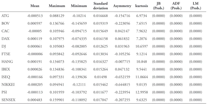
, respectively.

Table 2 presents the main descriptive statistics of each index return series, the Jarque-Bera tests of the normality of the series, the stationarity tests and the LM tests of Engle (1982) to the presence of heteroskedasticity.

The analysis of descriptive statistics allows us to draw the conclusion that only six of the 12 indexes had positive daily average return.

All series of returns, without exception, show signs of deviation from the normality hypothesis, as the coefficients of asymmetry and kurtosis are statistically different from a normal distribution (0 and 3, respectively). To confirm whether the fitting of the normal distribution is appropriate to the empirical distributions of the 12 series in all study periods, we also applied the Jarque-Bera backtesting. Taking into account the respective associated probabilities (equal to 0), we concluded that all series are statistically significant at 1%, clearly rejecting the hypothesis of normality thereof.

TABLE 2 – Descriptive statistics of the series

  Mean Maximum Minimum Standard

deviation Asymmetry kurtosis JB (Prob.)

ADF (Prob.)

LM (Prob.)

ATG -0.000513 0.088129 -0.10214 0.016668 -0.154716 6.9734 (0.0000) (0.0000) (0.0000)

BOV 0.000597 0.136766 -0.145659 0.019319 -0.223056 7.6515 (0.0000) (0.0000) (0.0000)

CAC -0.00005 0.105946 -0.094715 0.015649 0.042147 7.9632 (0.0000) (0.0000) (0.0000)

DAX 0.000119 0.107975 -0.074335 0.016158 0.061832 7.2076 (0.0000) (0.0000) (0.0000)

DJ 0.000061 0.105083 -0.082005 0.012625 0.031963 10.6597 (0.0000) (0.0000) (0.0000)

FTSE -0.000006 0.093842 -0.092646 0.013034 -0.105256 9.1214 (0.0000) (0.0000) (0.0000)

HANG 0.000191 0.134073 -0.135825 0.016327 -0.007715 10.848 (0.0000) (0.0000) (0.0000)

IBEX 0.000026 0.134836 -0.108341 0.015264 0.047132 9.5441 (0.0000) (0.0000) (0.0000)

ISEQ -0.000166 0.097331 -0.139636 0.01498 -0.652159 11.0664 (0.0000) (0.0000) (0.0000)

NIKKEI -0.000205 0.094941 -0.12111 0.015462 -0.644815 9.0135 (0.0000) (0.0000) (0.0000)

PSI -0.000113 0.101959 -0.103792 0.011677 -0.223954 12.9958 (0.0000) (0.0000) (0.0000)

SENSEX 0.000483 0.159901 -0.118092 0.017047 -0.207255 9.6325 (0.0000) (0.0000) (0.0000)

In order to determine the non-stationarity or integration of the series, we applied the traditional ADF test. The null hypothesis of the test states that the series have a unit root, i.e., that the series are integrated of order 1, versus the alternative hypothesis that the series do not have a unit root. The results confirm that the values of the probabilities of the tests of the 12 series do not exceed 1%, and clearly rejects the null hypothesis of integration of the series, and concludes that they show stationary or are I (0).

To t e s t t h e e x i s t e n c e o f c o n d i t i o n a l heteroskedasticity (ARCH effects), the rates of return of the indexes, autoregressive processes of first order were estimated, and LM tests of Engle (1982) were applied, to lag 20, residuals of autoregressive processes. In all cases, the probabilities of the LM tests allow us to conclude that, for a significance level of 1%, the series of rates of return indexes exhibit conditional heteroskedasticity, so the use of GARCH-type models proves adequate.

3.2 Empirical results

To assess the performance of VaR models in capturing the risk of the 12 markets studied,

we considered a theoretical investment portfolio, equally weighted, from which various multivariate conditional heteroskedasticity models were estimated, namely the VECH, BEKK and CCC specifications, for normal t-student distributions, and the asymmetrical effect, and on which VaR estimates were based. Finally, the EVT was applied in the three specifications for GARCH and Threshold GARCH (TGARCH) models, in order to incorporate the asymmetrical effect, and the normal and t-student distributions, in order to understand if it responds adequately to extreme variances that characterized the period studied. In all such cases, the estimates of VaR models considered confidence levels of 5%, 1% and 0.5%. The first confidence level follows the RiskMetrics methodology, the second on takes into account the requirements of the Basel II Committee, whereas the third one was chosen in order to realize the consequence of a more demanding estimate condition.

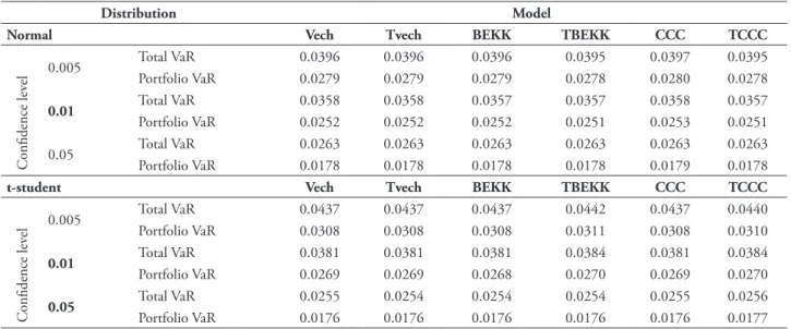
Table 3 compares total VaR of the various indexes with the portfolio’s VaR for the different estimate models and for the three confidence levels.

TABLE 3 – Comparison between portfolio var and total VaR estimates of indexes

Distribution Model

Normal Vech Tvech BEKK TBEKK CCC TCCC

Confidence lev

el 0.005

Total VaR 0.0396 0.0396 0.0396 0.0395 0.0397 0.0395

Portfolio VaR 0.0279 0.0279 0.0279 0.0278 0.0280 0.0278

0.01 Total VaR 0.0358 0.0358 0.0357 0.0357 0.0358 0.0357

Portfolio VaR 0.0252 0.0252 0.0252 0.0251 0.0253 0.0251

0.05 Total VaR 0.0263 0.0263 0.0263 0.0263 0.0263 0.0263

Portfolio VaR 0.0178 0.0178 0.0178 0.0178 0.0179 0.0178

t-student Vech Tvech BEKK TBEKK CCC TCCC

Confidence lev

el 0.005

Total VaR 0.0437 0.0437 0.0437 0.0442 0.0437 0.0440

Portfolio VaR 0.0308 0.0308 0.0308 0.0311 0.0308 0.0310

0.01 Total VaR 0.0381 0.0381 0.0381 0.0384 0.0381 0.0384

Portfolio VaR 0.0269 0.0269 0.0268 0.0270 0.0269 0.0270

0.05 Total VaR 0.0255 0.0254 0.0254 0.0254 0.0255 0.0256

Portfolio VaR 0.0176 0.0176 0.0176 0.0176 0.0176 0.0177

Notes: VaR estimates presented in the table were obtained from the variance-covariance matrix of GARCH models, without asymmetric effect (VECH, BEKK and CCC) and asymmetric effect (TVECH, TBEKK and TCC), considering the confidence intervals of 99.5% (0.5) 99% (1) 95% (5).

In all cases compared, the VaR of the portfolio is clearly lower than total individual VaR’s indexes. Therefore, there seems to be a reason to believe that market risk can be mitigated by means of diversification. Although the markets tend to linked closer and closer, the option for an investment strategy is based on the assumption of international diversification, which considers a broad set of markets, may constitute a form of protection against market risk.

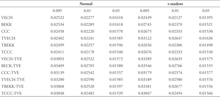
Table 4 presents the mean of VaR estimates of the various models. The most obvious feature is that the mean values depend more on the

distribution considered than on the forecast of the covariance matrix. In most cases, the mean VaR estimates, produced based on the t-student distribution, exceed those resulting from normal distribution, especially in the confidence levels of 0.5% and 1%. Only VECH and TVECH-EVT models, these two confidence levels, and the TCCC-EVT model, the confidence level of 0.5%, do not support this superiority. For the highest quantile, the conclusion is contrary, revealing superiority of estimates based on the normal distribution, in 67% of cases.

TABLE 4 – Mean estimates of VaR models

Normal t-student

0.005 0.01 0.05 0.005 0.01 0.05

VECH 0.02522 0.02277 0.01610 0.02439 0.02127 0.01395

BEKK 0.02534 0.02289 0.01618 0.02745 0.02370 0.01521

CCC 0.02458 0.02220 0.01570 0.02675 0.02333 0.01530

TVECH 0.02482 0.02241 0.01585 0.03122 0.02647 0.01636

TBEKK 0.02499 0.02257 0.01596 0.02656 0.02306 0.01498

TCCC 0.02411 0.02178 0.01540 0.02676 0.02333 0.01530

VECH-TVE 0.03092 0.02522 0.01572 0.03289 0.02635 0.01575

BECK-TVE 0.03409 0.02705 0.01580 0.03546 0.02766 0.01555

CCC-TVE 0.03139 0.02542 0.01557 0.03179 0.02574 0.01577

TVECH-TVE 0.03200 0.02590 0.01585 0.03189 0.02580 0.01576

TBEKK-TVE 0.03068 0.02520 0.01597 0.03381 0.02677 0.01556

TCCC-TVE 0.03048 0.02482 0.01539 0.03047 0.02494 0.01566

Notes: VaR estimates presented in the table were obtained from the variance-covariance matrix of GARCH models, without asymmetric effect (VECH, BEKK, CCC) and asymmetric effect (TVECH, TBEKK and TCC) and EVT, considering the confidence intervals of 99.5% (0.5) 99% (1) 95% (5).

Source: Author.

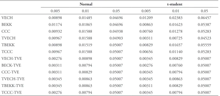
Table 5 summarizes the failure rate of various estimate models, i.e., the percentage of times the VaR estimates were exceeded by daily returns as a result of the unexpected market events. The results presented in this table reveal that the models that do not resort to extreme value theory, whether on the assumption of normal distribution or t-student distribution, generally showed difficulties in adapting to extreme changes in market.

In the case of estimates based on GARCH-type models, only the highest level of confidence, in the normal distribution, produces a failure rate

The use of the extreme value theory leads to different conclusions from those listed above, about the multivariate GARCH models. Estimates of GARCH models and TGARCH models, based on the two distributions, provide identical conclusions, with percentages of

exceptions below levels of confidence of 0.5% and 1%, contrary to what happens to the confidence level of 5 %. This fact gives a first indication of the superiority of the extreme value theory compared to the other methods, as we shall confirm with the implementation of a performance test.

TABLE 5 – Failure rate of VaR models

Normal t-student

0.005 0.01 0.05 0.005 0.01 0.05

VECH 0.00898 0.01485 0.04696 0.01209 0.02383 0.06457

BEKK 0.01174 0.01865 0.04696 0.00863 0.01623 0.05387

CCC 0.00932 0.01588 0.04938 0.00760 0.01278 0.05283

TVECH 0.00967 0.01588 0.04903 0.00311 0.00725 0.04523

TBEKK 0.00898 0.01519 0.05007 0.00829 0.01657 0.05559

TCCC 0.00967 0.01588 0.05007 0.00656 0.01140 0.05283

VECH-TVE 0.00276 0.00898 0.05007 0.00345 0.00829 0.05007

BECK-TVE 0.00311 0.00794 0.05007 0.00276 0.00760 0.05007

CCC-TVE 0.00311 0.00829 0.05007 0.00345 0.00794 0.05007

TVECH-TVE 0.00345 0.00863 0.05007 0.00345 0.00863 0.05007

TBEKK-TVE 0.00345 0.00863 0.05007 0.00311 0.00829 0.05007

TCCC-TVE 0.00276 0.00794 0.05007 0.00345 0.00794 0.05007

Notes: VaR estimates presented in the table were obtained from the variance-covariance matrix of GARCH models, without asymmetric effect (VECH, BEKK, CCC) and asymmetric effect (TVECH, TBEKK and TCC) and EVT, considering the confidence intervals of 99.5% (0.5) 99% (1) 95% (5).

Source: Author.

After estimating the different VaR models, Backtesting procedures were applied in order to reach a conclusion on the ability of these models to effectively manage the market risk of the stock markets. Firstly, we considered the unconditional coverage test or Kupiec test, which is a development of the failure rate, set by the Basel Committee, to oversee Banking activities. Secondly, the independence test was applied to test whether exceptions are IID. Finally, we applied the conditional coverage test, or Christoffersen test. Backtesting results are presented in tables 6 to 13.

In the unconditional coverage test and for two smaller quantiles, the t-student distribution showed better performance than the normal distribution. In both distributions, the

TABLE 6 – Backtesting results - GARCH model and normal distribution assumption.

VECH (0.5%)

VECH (1%)

VECH (5%)

BEKK (0.5%)

BEKK (1%)

BEKK (5%)

CCC (0.5%)

CCC (1%)

CCC (5%)

T₀ 2870 2853 2760 2862 2842 2760 2869 2850 2753

T₁ 26 43 136 34 54 136 27 46 143

T₀₀ 2844 2810 2636 2830 2793 2642 2842 2805 2625

T₀₁ 26 43 124 32 49 118 27 45 128

T₁₀ 26 43 124 32 49 118 27 45 128

T₁₁ 0 0 12 2 5 18 0 1 15

p 0.009 0.015 0.047 0.012 0.019 0.047 0.009 0.016 0.049

π₀₁ 0.009 0.015 0.045 0.011 0.017 0.043 0.009 0.016 0.046

π₁₁ 0.000 0.000 0.088 0.059 0.093 0.132 0.000 0.022 0.105

LR_uc 7.443 5.983 0.574 19.137 17.431 0.574 8.660 8.592 0.024

(0.006) (0.014) (0.449) (0.000) (0.000) (0.449) (0.003) (0.003) (0.878)

LR_ind 0.471 1.296 4.415 18.613 8.663 20.192 0.508 0.092 7.696

(0.492) (0.255) (0.036) (0.000) (0.003) (0.000) (0.476) (0.761) (0.006)

LR_cc 7.914 7.280 4.989 37.750 26.093 20.766 9.168 8.684 7.719

(0.019) (0.026) (0.083) (0.000) (0.000) (0.000) (0.010) (0.013) (0.021)

Notes: This table presents the results of the unconditional coverage (LRuc), independence (LRind) and conditional coverage (LRcc) tests of a portfolio comprising 12 indexes and VaR estimates, obtained from the variance-covariance matrix of the GARCH-VECH GARCH-BEKK and GARCH-CCC models, assuming that returns are described by normal distribution and considering confidence intervals of 99.5% (0.5), 99% (1) and 95% (5). The values in brackets refer to the probability of each test.

Source: Author.

TABLE 7 – Backtesting results - GARCH model and t-student distribution assumption.

VECH (0.5%)

VECH (1%)

VECH (5%)

BEKK (0.5%)

BEKK

(1%) BEKK (5%) CCC (0.5%) CCC (1%) CCC (5%)

T₀ 2861 2827 2709 2871 2849 2740 2874 2859 2743

T₁ 35 69 187 25 47 156 22 37 153

T₀₀ 2828 2762 2547 2847 2807 2607 2852 2824 2606

T₀₁ 33 65 162 24 42 133 22 35 137

T₁₀ 33 65 162 24 42 133 22 35 137

T₁₁ 2 4 25 1 5 23 0 2 16

π 0.012 0.024 0.065 0.009 0.016 0.054 0.008 0.013 0.053

π₀₁ 0.012 0.023 0.060 0.008 0.015 0.049 0.008 0.012 0.050

π₁₁ 0.057 0.058 0.134 0.040 0.106 0.147 0.000 0.054 0.105

LR_uc 20.887 40.292 11.903 6.304 9.552 0.890 3.384 2.073 0.480

(0.000) (0.000) (0.001) (0.012) (0.002) (0.345) (0.066) (0.150) (0.488)

LR_ind 3.207 2.570 12.562 1.549 11.136 20.192 0.337 2.845 6.921

(0.073) (0.109) (0.000) (0.213) (0.001) (0.000) (0.562) (0.092) (0.009)

LR_cc 24.094 42.862 24.465 7.852 20.687 21.082 3.721 4.918 7.402

(0.000) (0.000) (0.000) (0.020) (0.000) (0.000) (0.156) (0.086) (0.025)

Notes: This table presents the results of the unconditional coverage (LRuc), independence (LRind) and conditional coverage (LRcc) tests of a portfolio comprising 12 indexes and VaR estimates, obtained from the variance-covariance matrix of the GARCH-VECH GARCH-BEKK and GARCH-CCC models, assuming that returns are described by t-Student distribution and considering confidence intervals of 99.5% (0.5), 99% (1) and 95% (5). The values in brackets refer to the probability of each test.

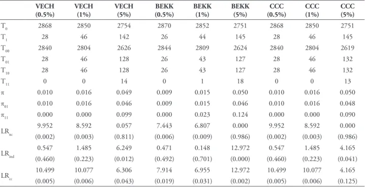
TABLE 8 – Backtesting results - TGARCH model and normal distribution assumption.

VECH (0.5%)

VECH (1%)

VECH (5%)

BEKK (0.5%)

BEKK (1%)

BEKK (5%)

CCC (0.5%)

CCC (1%)

CCC (5%)

T₀ 2868 2850 2754 2870 2852 2751 2868 2850 2751

T₁ 28 46 142 26 44 145 28 46 145

T₀₀ 2840 2804 2626 2844 2809 2624 2840 2804 2619

T₀₁ 28 46 128 26 43 127 28 46 132

T₁₀ 28 46 128 26 43 127 28 46 132

T₁₁ 0 0 14 0 1 18 0 0 13

π 0.010 0.016 0.049 0.009 0.015 0.050 0.010 0.016 0.050

π₀₁ 0.010 0.016 0.046 0.009 0.015 0.046 0.010 0.016 0.048

π₁₁ 0.000 0.000 0.099 0.000 0.023 0.124 0.000 0.000 0.090

LR_uc 9.952 8.592 0.057 7.443 6.807 0.000 9.952 8.592 0.000

(0.002) (0.003) (0.811) (0.006) (0.009) (0.986) (0.002) (0.003) (0.986)

LR_ind 0.547 1.485 6.249 0.471 0.148 12.972 0.547 1.485 4.165

(0.460) (0.223) (0.012) (0.492) (0.701) (0.000) (0.460) (0.223) (0.041)

LR_cc 10.499 10.077 6.306 7.914 6.955 12.972 10.499 10.077 4.165

(0.005) (0.006) (0.043) (0.019) (0.031) (0.002) (0.005) (0.006) (0.125)

Notes: This table presents the results of the unconditional coverage (LRuc), independence (LRind) and conditional coverage (LRcc) tests of a portfolio comprising 12 indexes and VaR estimates, obtained from the variance-covariance matrix of the Threshold GARCH (VECH, BEKK and CCC) models, assuming that returns are described by normal distribution and considering confidence intervals of 99.5% (0.5), 99% (1) and 95% (5). The values in brackets refer to the probability of each test.

Source: Author.

TABLE 9 – Backtesting results - TGARCH model and t-student distribution assumption.

VECH (0,5%)

VECH (1%)

VECH (5%)

BEKK (0.5%)

BEKK (1%)

BEKK (5%)

CCC (0.5%)

CCC (1%)

CCC (5%)

T₀ 2887 2875 2765 2872 2848 2735 2877 2863 2743

T₁ 9 21 131 24 48 161 19 33 153

T₀₀ 2878 2854 2645 2848 2805 2596 2858 2830 2606

T₀₁ 9 21 120 24 43 139 19 33 137

T₁₀ 9 21 120 24 43 139 19 33 137

T₁₁ 0 0 11 0 5 22 0 0 16

π 0.003 0.007 0.045 0.008 0.017 0.056 0.007 0.011 0.053

π₀₁ 0.003 0.007 0.043 0.008 0.015 0.051 0.007 0.012 0.050

π₁₁ 0.000 0.000 0.084 0.000 0.104 0.137 0.000 0.000 0.105

LR_uc 2.411 2.444 1.428 5.245 10.554 1.844 1.291 0.545 0.480

(0.121) (0.118) (0.232) (0.022) (0.001) (0.174) (0.256) (0.460) (0.488)

LR_ind 0.056 0.307 3.888 0.401 10.751 15.844 0.251 0.761 6.921

(0.813) (0.580) (0.049) (0.527) (0.001) (0.000) (0.616) (0.383) (0.009)

LR_cc 2.467 2.750 5.316 5.646 21.305 17.688 1.542 1.306 7.402

(0.291) (0.253) (0.070) (0.059) (0.000) (0.000) (0.463) (0.521) (0.025)

Notes: This table presents the results of the unconditional coverage (LRuc), independence (LRind) and conditional coverage (LRcc) tests of a portfolio comprising 12 indexes and VaR estimates, obtained from the variance-covariance matrix of the Threshold GARCH (VECH, BEKK and CCC) models, assuming that returns are described by t-Student distribution and considering confidence intervals of 99.5% (0.5), 99% (1) and 95% (5). The values in brackets refer to the probability of each test.

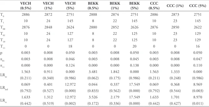
TABLE 10 – Backtesting results – GARCH-EVT model and normal distribution assumption.

VECH (0.5%)

VECH (1%)

VECH (5%)

BEKK (0.5%)

BEKK (1%)

BEKK (5%)

CCC (0.5%)

CCC (1%)

CCC (5%)

T₀ 2888 2870 2751 2887 2873 2751 2887 2872 2751

T₁ 8 26 145 9 23 145 9 24 145

T₀₀ 2880 2844 2621 2878 2850 2625 2878 2848 2622

T₀₁ 8 26 130 9 23 126 9 24 129

T₁₀ 8 26 130 9 23 126 9 24 129

T₁₁ 0 0 15 0 0 19 0 0 16

π 0.003 0.009 0.050 0.003 0.008 0.050 0.003 0.008 0.050

π₀₁ 0.003 0.009 0.047 0.003 0.008 0.046 0.003 0.008 0.047

π₁₁ 0.000 0.000 0.103 0.000 0.000 0.131 0.000 0.000 0.110

LR_uc 3.481 0.316 0.000 2.411 1.333 0.000 2.411 0.911 0.000

(0.062) (0.574) (0.986) (0.121) (0.248) (0.986) (0.121) (0.340) (0.986)

LR_ind 0.044 0.471 7.200 0.056 0.368 15.192 0.056 0.401 8.969

(0.833) (0.492) (0.007) (0.813) (0.544) (0.000) (0.813) (0.527) (0.003)

LR_cc 3.526 0.788 7.200 2.467 1.701 15.192 2.467 1.312 8.970

(0.172) (0.675) (0.027) (0.291) (0.427) (0.001) (0.291) (0.519) (0.011)

Notes: This table presents the results of the unconditional coverage (LRuc), independence (LRind) and conditional coverage (LRcc) tests of a portfolio comprising 12 indexes and VaR estimates, obtained from the variance-covariance matrix of the GARCH (VECH, BEKK and CCC) and EVT models, assuming that returns are described by normal distribution and considering confidence intervals of 99.5% (0.5), 99% (1) and 95% (5). The values in brackets refer to the probability of each test.

Source: Author.

TABLE 11 – Backtesting results – GARCH-EVT model and t-student distribution assumption.

VECH (0.5%)

VECH (1%)

VECH (5%)

BEKK (0.5%)

BEKK (1%)

BEKK (5%)

CCC

(0.5%) CCC (1%) CCC (5%)

T₀ 2886 2872 2751 2888 2874 2751 2886 2873 2751

T₁ 10 24 145 8 22 145 10 23 145

T₀₀ 2876 2848 2624 2880 2852 2626 2876 2850 2622

T₀₁ 10 24 127 8 22 125 10 23 129

T₁₀ 10 24 127 8 22 125 10 23 129

T₁₁ 0 0 18 0 0 20 0 0 16

p 0.003 0.008 0.050 0.003 0.008 0.050 0.003 0.008 0.050

π₀₁ 0.003 0.008 0.046 0.003 0.008 0.045 0.003 0.008 0.047

π₁₁ 0.000 0.000 0.124 0.000 0.000 0.138 0.000 0.000 0.110

LR_uc 1.563 0.911 0.000 3.481 1.842 0.000 1.563 1.333 0.000

(0.211) (0.340) (0.986) (0.062) (0.175) (0.986) (0.211) (0.248) (0.986)

LR_ind 0.069 0.401 12.972 0.044 0.337 17.549 0.069 0.368 8.969

(0.792) (0.527) (0.000) (0.833) (0.562) (0.000) (0.792) (0.544) (0.003)

LR_cc 1.633 1.312 12.972 3.526 2.179 17.549 1.633 1.701 8.970

(0.442) (0.519) (0.002) (0.172) (0.336) (0.000) (0.442) (0.427) (0.011)

Notes: This table presents the results of the unconditional coverage (LRuc), independence (LRind) and conditional coverage (LRcc) tests of a portfolio comprising 12 indexes and VaR estimates, obtained from the variance-covariance matrix of the GARCH (VECH, BEKK and CCC) and EVT models, assuming that returns are described by t-Student distribution and considering confidence intervals of 99.5% (0.5), 99% (1) and 95% (5). The values in brackets refer to the probability of each test.

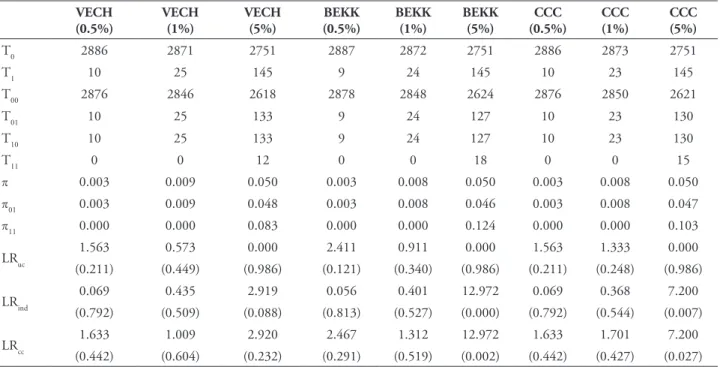
TABLE 12 – Backtesting results – TGARCH-EVT model and normal distribution assumption.

VECH

(0.5%) VECH (1%) VECH (5%)

BEKK (0.5%)

BEKK (1%)

BEKK (5%)

CCC (0.5%)

CCC (1%)

CCC (5%)

T₀ 2886 2871 2751 2886 2871 2751 2888 2873 2751

T₁ 10 25 145 10 25 145 8 23 145

T₀₀ 2876 2846 2618 2876 2846 2624 2880 2850 2619

T₀₁ 10 25 133 10 25 127 8 23 132

T₁₀ 10 25 133 10 25 127 8 23 132

T₁₁ 0 0 12 0 0 18 0 0 13

π 0.003 0.009 0.050 0.003 0.009 0.050 0.003 0.008 0.050

π₀₁ 0.003 0.009 0.048 0.003 0.009 0.046 0.003 0.008 0.048

π₁₁ 0.000 0.000 0.083 0.000 0.000 0.124 0.000 0.000 0.090

LR_uc 1.563 0.573 0.000 1.563 0.573 0.000 3.481 1.333 0.000

(0.211) (0.449) (0.986) (0.211) (0.449) (0.986) (0.062) (0.248) (0.986)

LR_ind 0.069 0.435 2.919 0.069 0.435 12.972 0.044 0.368 4.165

(0.792) (0.509) (0.088) (0.792) (0.509) (0.000) (0.833) (0.544) (0.041)

LR_cc 1.633 1.009 2.920 1.633 1.009 12.972 3.526 1.701 4.165

(0.442) (0.604) (0.232) (0.442) (0.604) (0.002) (0.172) (0.427) (0.125)

Notes: This table presents the results of the unconditional coverage (LRuc), independence (LRind) and conditional coverage (LRcc) tests of a portfolio comprising 12 indexes and VaR estimates, obtained from the variance-covariance matrix of the Threshold GARCH (VECH, BEKK and CCC) and EVT models, assuming that returns are described by normal distribution and considering confidence intervals of 99.5% (0.5), 99% (1) and 95% (5). The values in brackets refer to the probability of each test.

Source: Author.

TABLE 13 – Backtesting results – TGARCH-EVT model and t-student distribution assumption.

VECH (0.5%)

VECH (1%)

VECH (5%)

BEKK (0.5%)

BEKK (1%)

BEKK (5%)

CCC (0.5%)

CCC (1%)

CCC (5%)

T₀ 2886 2871 2751 2887 2872 2751 2886 2873 2751

T₁ 10 25 145 9 24 145 10 23 145

T₀₀ 2876 2846 2618 2878 2848 2624 2876 2850 2621

T₀₁ 10 25 133 9 24 127 10 23 130

T₁₀ 10 25 133 9 24 127 10 23 130

T₁₁ 0 0 12 0 0 18 0 0 15

π 0.003 0.009 0.050 0.003 0.008 0.050 0.003 0.008 0.050

π₀₁ 0.003 0.009 0.048 0.003 0.008 0.046 0.003 0.008 0.047

π₁₁ 0.000 0.000 0.083 0.000 0.000 0.124 0.000 0.000 0.103

LR_uc 1.563 0.573 0.000 2.411 0.911 0.000 1.563 1.333 0.000

(0.211) (0.449) (0.986) (0.121) (0.340) (0.986) (0.211) (0.248) (0.986)

LR_ind 0.069 0.435 2.919 0.056 0.401 12.972 0.069 0.368 7.200

(0.792) (0.509) (0.088) (0.813) (0.527) (0.000) (0.792) (0.544) (0.007)

LR_cc 1.633 1.009 2.920 2.467 1.312 12.972 1.633 1.701 7.200

(0.442) (0.604) (0.232) (0.291) (0.519) (0.002) (0.442) (0.427) (0.027)

Notes: This table presents the results of the unconditional coverage (LRuc), independence (LRind) and conditional coverage (LRcc) tests of a portfolio comprising 12 indexes and VaR estimates, obtained from the variance-covariance matrix of the Threshold GARCH (VECH, BEKK and CCC) and EVT models, assuming that returns are described by t-Student distribution and considering confidence intervals of 99.5% (0.5), 99% (1) and 95% (5). The values in brackets refer to the probability of each test.

The analysis of the temporal independence of exceptions revealed that the models generally reported good performance in the two lower quantiles. Only the BEKK model evidenced difficulty detecting exceptions in clusters, in particular in the normal distribution. Regarding the highest quantile, the models showed clear difficulty in identifying independence, and the TVECH-EVT model was the only one to prove the ability to capture the effect of independence, patent in both distributions. On the other hand, the comparison between both distributions translates into very similar results, with the normal distribution to validate 91.7%, 91.7% and 8.3% of models in quantiles 0.5%, 1% and 5%, respectively, whereas the t-Student distribution contributes to validate 100%, 83.3% and 8.3% of the models in each of said quantiles. These results allow the conclusion that none of the distributions has superiority over the other, and the models ability to test property of exceptions that are IID does not depend on the type of distribution considered.

The conditional coverage test, which combines the effects of unconditional coverage and independence, evidenced the superiority of models based on the t-student distribution compared to those based on the normal distribution, at the confidence levels of 0.5% and 1%, with acceptance at 83% and 75% of the cases for the two previous confidence levels, respectively, vis-à-vis the 50% acceptance in the normal distribution. For the highest level of confidence, the situation changes with the normal distribution (33.3%), which is higher than the t-student (16.7%), although in both cases the demonstrated performance has been very limited.

Several different models proved their inability as risk management instruments, at the three confidence levels, in particular models with the assumption of normal distribution (BEKK, CCC, and TVECH and TBEKK). This also happened with some models supported by the t-student distribution, as was the case

of VECH and BEKK models. Conversely, the TVECH (t-student), TVECH-EVT (normal and t-student) and TCCC-EVT (normal) models revealed consistent performances in the three quantiles. We should point out that the EVT led to a marked improvement in the performance of VaR models, especially in the lower two quantiles, with all the models inspired by this methodology passing the Christoffersen test. Regarding the highest confidence level, only TVECH and TCCC models showed good performance, the first in both distributions, and the second on in the normal distribution.

Results suggest that the most important element in the accuracy of estimates of VaR models is the use of EVT, whose theoretical genesis uses the generalized Pareto distribution. This situation highlights the importance of this approach, as a determining factor in the performance of the models, similar to results obtained by other authors – for example, Lopez and Walter (2001); in a second order of importance, the specification of the multivariate model appears.

Of the set of specifications considered in this study, the BEKK multivariate model clearly presented the worst performance, while the TVECH-EVT model stood out positively among the others, and was validated in all tests and in both distributions, revealing therefore its ability to incorporate the extreme conditions experienced in the markets, which marked the period considered in this study, as a consequence of the Dot-Com and global financial crises.

4 C O N C L U S I O N A N D F U T U R E

IMPLICATIONS

the covariance matrixes, generated by various multivariate conditional heteroskedasticity models, estimated in accordance with the normal and t-Student distributions, to predict the VaR, similarly to the methodologies used in other papers. Differently with respect to these papers, however, we suggested a new methodology that combines these models with the extreme values theory, as a VaR estimate methodology, in order to try to conveniently accommodate the high turbulence that characterized stock markets, including those representing European states under international financial assistance.

The comparison between the total VaR’s of the various indexes and the VaR of the investment portfolio allowed the conclusion that, in all events, the portfolio VaR is clearly inferior. This fact allows the opportunity to minimize market risk, when an investor bets on a strategy of international diversification. Although the link between stock markets is growing closer, a diversification strategy that considers a broad set of markets can be a form of investor protection against market risk.

The application of performance validation tests of VaR estimates reveals that the most important element in the accuracy of these estimates is the use of EVT, based on the generalized Pareto distribution. Then, in terms of importance, is the specification of the multivariate model. Of the set of specifications considered in this study, the BEKK multivariate model was clearly the worst in performance, whereas the TVECH-EVT model stood out positively from the others, and was validated in all tests and in both distributions. It revealed its ability to incorporate extreme market conditions experienced during the time period studied.

The results show that the methodology proposed in this paper can accommodate the high turbulence in the markets, and it can be seen as an appropriate option in the management of market risk.

In future work, it may be interesting to use an optimization model that considers, at the same level, market returns and risk estimates, and relate the multivariate GARCH to the EVT

models, in order to obtain additional information to international investors on their investment alternatives, taking into account the opportunities offered by emerging and developed markets.

REFERENCES

ANDREEV, V. O. et al. An application of EVT, GPD and POT methods in the russian stock

market (RTS index). Nov. 2009. Working Papers

Series. Disponível em: <http:// papers.ssrn.com/ sol3/papers.cfm?abstract_id=1507678>. Acesso em: 12 mar. 2013.

ANGELIDIS, T.; BENOS, A.; DEGIANNAKIS, S. The use of GARCH models in VaR estimation.

Statistical Methodology, [S. l.], v.1, n. 1-2,

p. 105-128, Dec. 2004.

ASSAF, A. Extreme observations and risk assessment in the equity markets of MENA region: tail measures and Value-at-Risk. International

Review of Financial Analysis, Amsterdam,

v. 18, n. 3. p. 109-116, June 2009.

BEST, P. Implementing Value-at-Risk. Chichester: John Wiley & Sons, 1998.

BOLLERSLEV, T. Modeling the coherence in the short-run nominal exchange rates: a multivariate generalized ARCH model. Review of Economics

and Statistics, Cambridge, v. 72, n. 3, p.

498-505, Aug. 1990.

______; ENGLE, R. F.; WOOLDRIDGE, J. M. A capital asset pricing model with time-varying covariances. Journal of Political Economy, Chicago, v.96, n. 1, p. 116-131, Feb. 1988. CAMPBELL, S. D. A review of backtesting

and backtesting procedures. 2005. Finance

CAPORIN, M.; MCALEER, M. Robust ranking of multivariate GARCH models by problem

dimension. June, 2012. Kyoto University/KIER

Working Papers 815.

CHRISTOFFERSEN, P. Elements of financial

risk management. Amsterdam: Academic Press,

2003.

DANIELSSON, J.; DE VRIES, C. G.

Value-at-Risk and extreme returns. 1997. Discussion

Paper 273 LSE Financial Markets Group, London School of Economics.

EMBRECHTS, P.; KLUPPERLBERG, C.; MIKOSCH, T. Modelling extreme events

for insurance and finance. Berlin, Germany:

Springer, 1997.

ENGLE, R. F. Autoregressive conditional hetereoskedasticity with estimates of the variance of United Kingdom inflation. Econometrica, Oxford, v. 50, n. 4 p. 987-1007, July 1982. ______; KRONER, K. F. Multivariate simultaneous generalised GARCH. Econometric Theory, Cambridge, v. 11, n. 1, p. 122-150, Mar. 1995. ESCH, L.; KIEFFER, R.; LOPEZ, T. Asset and

risk management: risk oriented finance. England:

Wiley Finance, 2005.

FERREIRA, M. A.; LOPEZ, J. A. Evaluating interest rate covariance models within a Value-at-Risk framework. Journal of Financial

Econometrics, Oxford, v. 3, n. 1, p. 126-168,

Winter 2005.

GIOT, P.; LAURENT, S. Value-at-risk for long and short trading positions. Journal of Applied

Econometrics, Chichester, v. 18, n. 6, p.

641-664, Nov./Dec. 2003.

HARRIS, R.; SOLLIS, R. Modelling and

forecasting financial time series. New York:

Wiley, 2003.

JORION, P. Value at risk: the new benchmark for managing financial risk. 3rd ed. United States: McGraw-Hill, 2007.

KUPIEC, P. H. Techniques for verifying the accuracy of risk management models. Journal of

Derivatives, [S. l.], v. 3, n. 2, p. 73-84, Winter

1995.

LOPEZ, J. A.; WALTER, C. A. Evaluating covariance matrix forecasts in a value-at-risk framework. Journal of Risk, London, v.3, p. 69-98, Apr. 2001.

MANGANELLI, S.; ENGLE, R. F. Value at risk

models in finance. Aug. 2001. European Central

Bank, Working Paper Nº 75, p.1-40.

MARKOWITZ, H. Portfolio selection. Journal

of Finance, Malden, v.7, n.1, p. 77-91, Mar.

1952.

MARIMOUTOU, V.; RAGGAD, B.; TRABELSI, A. Extreme value theory and Value at Risk: application to oil market. Energy Economics, Amsterdam, n. 31, p. 519-530, Feb. 2009. MCNEIL, A. J. Calculating quantile risk measures for financial return series using

extreme value theory. 1998. Department

Mathematik, ETH Institutional Repository, Zentrum, Zurich.

______. Extreme value theory for risk managers.

Internal modelling and CAD II. London: Risk

Books, 1999.

______; FREY, R. Estimation of tail-related risk measures for heteroscedastic financial time series: an extreme value approach. Journal of Empirical

Finance, Amsterdam, v.7, n. 3-4, p. 271-300,

Nov. 2000.

MORIMOTO, T.; KAWASAKI, Y. Empirical comparison of multivariate GARCH models

for estimation of intraday Value at Risk. 2008.

Disponível em: <http://dx.doi.org/ 10.2139/ssrn>. Acesso em: 02 maio 2013.

NIGUEZ, T. M. Volatility and VaR forecasting in the Madrid Stock Exchange. Spanish Economic

REISS, R. D.; THOMAS, M. Statistical analysis

of extreme values: with applications to insurance,

finance, hydrology and other fields. Basel, Switzerland: Birkhauser-Verlag, 1997.

SCHERRER, W.; RIBARITS, E. On the parameterization of multivariate GARCH models. Econometric Theory, Cambridge, v. 23, n. 3, p.464-484, Jun. 2007.

SO, M. K. P.; YU, P. L. H. Empirical analysis of GARCH models in value at risk estimation.

International Financial Markets, Institutions

and Money, Binghamton; Amsterdam, v. 16,

n. 2, p. 180-197, Apr. 2006.

TSAY, R. S. Analysis of financial time series. New Jersey: John Wiley & Sons, 2005.

WORLD BANK GROUP. c2014. Disponível em: <http://data.worldbank.org/indicator/ CM.MKT.LCAP.CD>. Acesso em: 02 maio 2013. WU, P. T.; SHIEH, S. J. Value-at-Risk analysis for long-term interest rate futures: Fat-tail and long memory in return innovations. Journal

of Empirical Finance, Amsterdam, v. 14, n. 2,