Universidade do Algarve
SPATIAL AND TEMPORAL VARIATION OF
COMMERCIALLY IMPORTANT BIVALVE SPECIES IN
THE ALGARVE COAST, PORTUGAL
Joana Maria Veloso Rodrigues Bento de Almeida
Dissertação para a obtenção do grau de Mestre em
Biologia Marinha
Universidade do Algarve
Spatial
and
temporal
variation
of
commercially important bivalve species, in the
Algarve coast, Portugal
Joana Maria Veloso Rodrigues Bento de Almeida
Dissertação para a obtenção do grau de Mestre em
Biologia Marinha
Trabalho efetuado sob a orientação de Dra. Margarida Castro (UAlg)
Dr. Miguel Gaspar (IPMA)
Spatial and temporal variation of commercially
important bivalve species, in the Algarve coast,
Portugal
Joana Maria Veloso Rodrigues Bento de Almeida©
Declaração de autoria de trabalho:
Declaro ser a autora deste trabalho, que é original e inédito. Autores e
trabalhos consultados estão devidamente citados no texto e constam da
listagem de referências incluída.
A Universidade do Algarve tem o direito, perpétuo e sem limites geográficos, de arquivar e publicitar este trabalho através de exemplares impressos reproduzidos em papel ou de forma digital, ou por qualquer outro meio conhecido ou que venha a ser inventado, de o divulgar através de repositórios científicos e de admitir a sua cópia e distribuição com objetivos educacionais ou de investigação, não comerciais, desde que seja dado crédito ao autor e editor.
i
Agradecimentos
Ao chegar ao final desta longa caminhada, que passou por muitos altos e baixos, e momentos de incerteza e cansaço, recordo todos os que estiveram ao meu lado e me ajudaram a conseguir concluir mais esta etapa da minha vida.
À minha orientadora de Tese, prof. Dra. Margarida Castro, obrigada por todo o apoio, pelo empenho na orientação deste projeto, pelo esclarecimento de dúvidas, e em especial pela sua paciência. Muito obrigada!
Ao Dr. Miguel Gaspar, agradeço a partilha de conhecimento e a simpatia com que sempre me acompanhou durante esta fase da minha vida académica, e contribuindo da melhor forma possível para o meu sucesso. Obrigada!
Ao IPMA, por me ter generosamente cedido os dados necessários à realização deste projeto. Obrigada!
Deixo um especial agradecimento à Marta Rufino, pela sua grande dedicação e contribuição ao longo do último ano, em que partilhou do seu tempo para me incentivar a fazer sempre melhor e alcançar os meus objetivos. Obrigada Marta!
Gostaria também de expressar a minha gratidão à Prof. Amélia Dill, por ter despendido do seu tempo para me ajudar a concretizar esta fase académica, sempre afável, disponível e disposta a ajudar. Tenho-a como um grande exemplo e estarei sempre grata por todo o seu apoio. Obrigada!
A todos os que se cruzaram comigo durante estes anos no Algarve, Colegas, Professores, Funcionários, foi um prazer trabalhar na vossa companhia, obrigada!
Ao meu irmão Bruno, que sem saber, me motivou a encarar estes últimos meses de frente e de cabeça erguida, mais motivada e focada na conclusão deste projeto. Obrigada!
Ao meu amor, Ricardo, que me acompanhou ao longo destes últimos dois anos, sem nunca deixar de acreditar em mim, de me ouvir e de me aturar nos momentos menos bons; que celebrou comigo as pequenas vitórias alcançadas ao longo deste percurso; que me viu desmotivar e vacilar e esteve sempre ao meu lado para me incentivar. Entre muitas razões para te agradecer, esta é uma delas, não o teria conseguido sem ti. Obrigada!
Aos meus pais, Helena e Jaime, que sempre me acompanharam e incutiram a força e a coragem necessária para crescer. É a vós que dedico a conclusão deste projeto, por me terem ensinado a nunca desistir, a superar-me sempre e a sonhar mais alto. Um especial agradecimento, do fundo do coração.
ii
Resumo
A pesca artesanal do Algarve é um setor muito importante para as comunidades locais e para a economia Algarvia. As espécies alvo desta pesca são a amêijoa-branca (Spisula
solida), o pé-de-burrinho (Chamelea gallina), a conquilha (Donax trunulus) e o
longueirão (Ensis siliqua). O Instituto Português do Mar e da Atmosfera (IPMA) é responsável pela gestão destas pescas e dos recursos existentes, para garantir o seu desenvolvimento sustentável. Sabe-se que para além da pressão da pesca exercida sobre estas populações de bivalves costeiros, existem fatores ambientais que influenciam o seu crescimento e sucesso reprodutivo. Este estudo teve como base as campanhas de monitorização destes bancos de bivalves, realizadas anualmente pelo IPMA, no período de 1999 a 2011, bem como os dados ambientais de precipitação, um indicador de disponibilidade de alimento (clorofila a), índice de vento e Sea surface Temperature (SST) ao longo destes 13 anos. Os objetivos deste estudo são o de analisar a variação da distribuição espacial e temporal destas espécies, no Barlavento e Sotavento Algarvio, bem como o de avaliar de que forma os parâmetros ambientais estudados condicionam a abundância das espécies em questão no ano seguinte, no período antes da desova e no período de desova + um mês. Para tal, foram elaborados mapas de distribuição anual, divididos em espécie e em região (Barlavento e Sotavento) e foram aplicados 16 modelos lineares abrangendo as quatro espécies em estudo, as duas regiões (Barlavento e Sotavento) e os dois períodos considerados (antes da desova e depois da desova+ um mês). Os resultados destes estudo demonstraram que a distribuição e a abundância destas espécies varia ao longo dos anos, revelando padrões distintos de formação dos bancos em termos de preferência ou ausência de cada espécie, e que todos os fatores ambientais estudados foram significativos na determinação da sua abundancia do ano seguinte. Os parâmetros ambientais mais significativos foram os níveis de precipitação e de clorofila a, especialmente na zona de Barlavento. No geral, o aumento dos níveis de clorofila a revelou-se benéfico na contribuição para a abundancia das espécies, enquanto adultos reprodutores bem como larvas em crescimento, enquanto os níveis de precipitação mais abundante se revelaram importantes no inverso, para as populações adultas, e prejudiciais no verão, para as fases iniciais de vida destes bivalves. Este estudo revela ainda a necessidade de se aprofundar o conhecimento sobre a interligação dos parâmetros ambientais estudados com as características específicas da costa Algarvia, para contribuir para uma melhor gestão das pescas e previsão antecipadas das medidas necessárias à manutenção destas importantes comunidades de bivalves.
iii
Abstract
Artisanal fisheries in the Algarve are a very important industry for local communities and for the local economy. The target species in this fishery are the white clam (Spisula
solida), the striped venus (Chamelea gallina), the donax clam (Donax trunulus) and
razor clam (Ensis siliqua). The Portuguese Institute of the Sea and Atmosphere (IPMA) is responsible for the management of these fisheries and the existing resources, to ensure its sustainable development. It is known that in addition to the fishing pressure exerted on these coastal bivalve populations, there are environmental factors that influence their growth and reproductive success. This study was based on the monitoring campaigns of these bivalve banks, held annually by the IPMA, from 1999 to 2011, as well as environmental data of rainfall, an indicator of food availability (chlorophyll a), wind index and Sea surface Temperature (SST) over these 13 years. The objectives of this study are to analyze the variation of the spatial and temporal distribution of these species in the Western and Eastern Algarve, as well as to evaluate how the studied environmental parameters condition the abundance of the species concerned, in the following year, for the period before spawning and for the period after spawning + one month. Thus, annual distribution maps were elaborated for each species and region (Western and Eastern) and 16 linear models were applied to all four studied species, the two regions (Barlavento and Sotavento) and the study period ( three months before spawning and spawning + one month The results of this study showed that the distribution and abundance of these species varies over the years, revealing different patterns of banks in terms of preference or absence for each species, and that all the analyzed environmental factors were significant in determining their abundance, the following year. The most significant environmental parameters affecting abundance were the rainfall and the chlorophyll a levels, especially in the Western area. In general, increasing chlorophyll levels were beneficial in contributing to the abundance of species either breeding adults or growing larvae, while the most abundant rainfall levels were positive for adult populations, and negative to the early life stages of these bivalves. This study also shows the need to develop a better understanding of the relationship between the environmental parameters studied and the specific characteristic of the Algarve coast, so there can be a better management of the stocks, and an anticipated prediction of the populations’ growth, which will enable a better monitoring of these important bivalve communities.
iv GENERAL INDEX. Agradecimentos ... i Resumo ... ii Abstract ... iii Index... iv Figure Index... vi
Table Index ... vii
1 Introduction ... 1
1.1 Population dynamics ... 1
1.2 Artisanal bivalves fisheries in Portugal ... 2
1.3 Target species ... 3
Spisula solida ... 3
Donax trunculus ... 4
Chamelea gallina ... 5
Ensis siliqua ... 5
1.4 Monitoring bivalve stocks in coastal areas ... 6
2 Material and methods ... 8
2.1 Study site ... 8
2.2 Abundance data ... 9
2.3 Data treatment ... 10
v Environmental variables ... 12 Statistical analysis ... 14 3 Results ... 16 3.1 Spatial distribution ... 16 3.2 Environmental variables... 25 3.3 Statistical analysis ... 28 4 Discussion ... 32
4.1 Species spatial distribution ... 32
4.2 Influence of environmental parameters... 33
Spisula solida ... 33 Donax trunculus ... 34 Chamelea gallina ... 35 Ensis siliqua ... 36 5 References... 39 Annex 1………...………49
vi
Figure Index
Fig. 2.1- Study area ... 9
Fig. 2.2- sampling stations in Barlavento and Sotavento ... 10
Fig. 2.3- Example of a Post map for Chamelea gallina abundance in Barlavento (2005) ... 11
Fig. 2.4- Example of a Shape file for Chamelea gallina abundance in Barlavento (2005) ... 11
Figure 2.5- wind index values ... 13
Fig. 3.1 – S solida spatial variation in Barlavento and Sotavento from 1999 to 2005 ... 17
Fig. 3.2 - S solida spatial variation in Barlavento and Sotavento from 2006 to 2011 ... 18
Fig. 3.3- D. trunculus spatial variation in Barlavento and Sotavento from 1999 to 2005 ... 19
Fig. 3.4- D. trunculus spatial variation in Barlavento and Sotavento from 2006 to 2011 ... 20
Fig. 3.5- – C. gallina spatial variation in Barlavento and Sotavento from 1999 to 2005 ... 21
Fig. 3.6- C. gallina spatial variation in Barlavento and Sotavento from 2006 to 2011 ... 22
Fig. 3.7- E. siliqua spatial variation in Barlavento and Sotavento from 1999 to 2005 ... 23
Fig. 3.8- E. siliqua spatial variation in Barlavento and Sotavento from 2006 to 2011 ... 24
Fig. 3.9- Mean monthly SST variation in Barlavento between Jan 1998 and Dec 2010 ... 25
Fig. 3.10- Mean monthly SST variation in Sotavento between Jan 1998 and Dec 2010 ... 25
Fig. 3.11- Mean monthly chlorophyll a variation in Barlavento between Feb 2000 and Dec 2010 ... 26
Fig. 3.12- Mean monthly chlorophyll a variation in Sotavento between Feb 2000 and Dec 2010 ... 26
Fig. 3.13- Mean monthly precipitation between Jan 1998 and Dec 2010 ... 27
Fig. 3.14- Mean monthly wind index variation in Barlavento between Jan 1998 and Dec 2010 ... 28
vii
Table index
Table 2.1- Spawning period of the studied species ... 15
Table 3.1- Statistical results for the model ‘3 months before spawning’ ... 29
Table 3.2- Statistical results for the model ‘spawning + 1 month’ ... 30
1
1 Introduction
The class Bivalvia is composed of around 9200 living species, which ranks it as the second largest class in the Phylum Mollusca (Huber, 2010), and therefore extremely diversified. Bivalve benthic populations constitute an important component of coastal ecosystems and have increasingly become focus of research. These animals are low on the food web and represent a major source of food for numerous predators and a vast resource for human consumption (Dame, 1993). Their feeding strategy (suspension-feeding or filter-(suspension-feeding) is responsible for the cycling and feedback of essential elements back into the water column (Dame & Olenin, 2005). Due to short life cycles and pelagic larvae, bivalves respond quickly to environmental changes and can be used as indicators of temperate coastal waters variations (Zeichen et al., 2002).
As filter-feeders, they remove large amounts of suspended material from the water; furthermore, they absorb heavy elements by ingestion of food or water, and have been established as bioindicators for monitoring the concentration of heavy trace metals in many areas of the world (Shpigel, 2005, Özden et al., 2009). There has also been an increasing interest is using bivalves as bioremediators of the eutrofication in estuaries (Shpigel, 2005; Carmichael et al., 2012). Benthic communities are mostly sessile and therefore considered to be a tool in monitoring long-term changes in the marine ecosystem (Grémare et al., 1998).
1.1 Population dynamics
The reproductive activity of bivalves is controlled by the interaction between endogenous and environmental factors (Normand et al., 2008; Enríquez-Díaz et al., 2009), but has not yet been fully understood. Over 70% of the benthic invertebrates go through a planktonic life stage during their larval development (Thorson, 1950), followed by the adult benthic stages. Thus, abundance, distribution and age-structure of the populations are strongly dependent on the coupling of these two stages (Alexander and Roughgarden, 1996 ; Menge et al., 1997).
Among other factors, larval supply of intertidal species can vary depending on wind stress and direction, spring and neap tidal cycles, periods of upwelling and downwelling events, or according to the local hydrodynamic regime, including the influence of
2 riverine input flushing times and local turbulence (Chícharo & Chícharo, 2001; Shanks, 2009; Porri et al., 2008). A study conducted by Thomas et al (2012) in the deep Ahe atoll lagoon and showed larvae displayed a significant dispersal capacity at the lagoon scale, especially with dominant eastern winds. R. decussatus larvae abundances in Ria Formosa coastal lagoon have been significantly correlated with wind velocity and tidal amplitude (Chícharo & Chícharo, 2001).
Settlement has been defined as the integration of juveniles in a population (Connell, 1985), and is one of the main processes governing temporal variations and spatial structure of the adult populations (Ellien et al., 2004). Research on the relationship between stock size and recruitment and its role in determining sustainable yields has had a long controversial history (Maunder & Deriso, 2013). Debate still remains about the relative importance of the environment versus spawning biomass in determining recruitment. For example, Myers et al. (1999) conducted a meta-analysis of the steepness of the stock–recruitment model for a wide range of species, identifying that spawning biomass determined recruitment for many species, at least at low spawner abundance.
1.2 Artisanal bivalves fisheries in Portugal
Artisanal fisheries promote economic development by generating considerable employment and are source of income for communities (Guyader et al., 2013).Artisanal fisheries represent over 50% of the fish caught for human consumption (FAO, 2010 p.70), and constitute a substantial foundation of the Portuguese social and cultural tradition. One of the most important artisanal fisheries in Portugal is the catch of coastal molluscs (mostly bivalves), which has become an important commercial enterprise, especially in the South coast. Both the high economic value and high volume of bivalve landings, combined with the number of fishermen, the number of vessels and high employment related to the subject, makes the Algarve artisanal fleet most significant in the sector (Chícharo et al., 2002; Gaspar et al., 2003; Oliveira et al., 2009; Vânia et al., 2014;).
In Portugal, monitoring, managing and assessing of fisheries is controlled by the Portuguese Institute of the Ocean and Atmosphere (IPMA). In 1986, IPMA introduced a seasonal closure, allowing bivalves to grow to a more marketable size and reproduce at
3 least once before capture (Gaspar et al., 1998; Gaspar et al., 2013). The seasonal closure is now set from May 1 to June 15 (Gaspar & Chícharo, 2007) but they can change according to the stock condition each year. In the South sector, the fishery is not managed by weekly fishing quotas per vessel, but by daily fishing quotas established per vessel and depending on species (Oliveira et al., 2013).The only harvest limitations for coastal bivalves are size limits and the daily quota (Gaspar et al., 1999, 2003). Based on their scientific studies, IPMA proposed adjustments to the technical characteristics of the fishing gear, such as minimum mesh sizes and maximum tooth spacing among others, to adjust to target species ecology (Gaspar et al., 2002). As a result, in the South bivalve fisheries, only mechanical dredges with a rigid iron structure connected to a lower bar with teeth attached to a metallic grid box for collection are permitted (Gaspar et al., 2003). This dredge that can penetrate into the sediment for up to 50 cm, depending on target species and sediment type (Gaspar et al., 1999; Chícharo
et al., 2002). Boats are allowed to work with two dredges (Gaspar et al., 2003; Oliveira et al., 2010).
1.3 Target species
The south coast of Portugal hosts a mixture of bivalve species mostly from tropical (from North Africa), temperate (from north Atlantic) and Mediterranean characteristics (Rufino et al., 2008). The target species of the dredge fleet along the Algarve coast are the surf clam (Spisula solida), the Donax clam (Donax trunculus), the striped venus clam (Chamelea gallina) and the razor clam (Ensis siliqua) (Gaspar al., 1998; Chícharo
et al., 2002) which constitute the species used in the present work. Spisula solida
The white clam S. solida (Linnaeus, 1758) is one of the most commercially important species in Portugal. It inhabits mainly sandy bottoms from Iceland and the Norwegian Sea to the Iberian Peninsula, Morocco and Madeira islands, and is most commonly found at depth between 3 and 13m (Gaspar et al., 1995). Baptista & Leitão (2014) observed a depth distinct distribution pattern of S solida in the Algarve.
4 Joaquim et al. (2008) studied the reproductive cycle of S. solida in the Algarve in 2003 and their major findings were that the spawning period began in late winter as a response in sea water temperature (SST) increase, and lasted through spring. In summer the species was found in resting period. Gametogenic activity began in September as a consequence of decreasing temperature. More accurately, Gaspar et al. (1996) describes the spawning period between the months of March and May. Dolbeth et al., (2006) suggests benthic recruitment of this species in June for the study area.
Donax trunculus
D. trunculus is a warm water suspension-feeder distributed throughout the
Mediterranean and the Atlantic from France to Senegal (Ramon et al., 1995; Tlili et al., 2010; de la Huz et al., 2002) and commonly inhabits the intertidal and shallow subtidal zone of exposed sandy beaches along European and North African coasts (Gaspar et al., 1999; de la Huz et al., 2002). They represent the most inshore species of surf clam in Portugal, commonly found at depths between 0 and 3m depth, well adapted to the swash zone (Gaspar et al., 1999). This species been used as a sentinel species for biomonitoring in environmental assessments (Tlili et al., 2010).
Their reproductive cycle has been studied in the Mediterranean (Ramon et al., 1995) in the Adriatic coast (Zeichen et al., 2002) and in the south coast of Portugal (Gaspar et
al., 1999) and differences are relevant. The longevity of D. trunculus in the Atlantic is
about 5 years, longer than in the Mediterranean (Ramon et al., 1995; Zeichen et al., 2002). A bimodal recruitment in Donax trunculus appears to be characteristic of the Mediterranean populations, whereas in the Atlantic populations there is always a single annual recruitment (Gaspar et al., 1999; Ramon et al., 1995). Moreover, the Atlantic populations of D. trunculus occur intertidally and are exposed to lower seawater temperatures than the subtidal Mediterranean populations. Gaspar et al. (1999) monitored gonadal development in D. trunculus and concluded the spawning occurred between March and August with two major spawning phases: the first in March and the second between May and August, and in their first year of life, they reach sexual maturity. Depth segregation between juveniles and adults was reported (Zeichen et al., 2002; Rufino et al., 2010).
5
Chamelea gallina
C. gallina (Linnaeus, 1758) is an infaunal bivalve species that occurs in the infralittoral
zone (Gaspar et al., 2004) on the eastern Atlantic coast, Norway and the British Isles, Iberian Peninsula, Morocco, Madeira, and the Canary Islands, the Mediterranean Sea, the Black Sea and the Adriatic Sea (Poppe & Goto, 1993; Tebble, 1966).
It is distributed along clean sandy bottoms at depths between 3m and 24m (Gaspar & Monteiro, 1993). It is intensively exploited in Europe, mainly in the United Kingdom, Ireland, Spain, and Portugal (Gaspar & Monteiro 1998; Arias-Perez et al., 2012) and is regarded as an increasingly valuable fishery resource (Cross et al., 2014).
Their reproductive cycle in the Algarve was studied by Gaspar & Monteiro (1998) where gametogenesis begins in November and a single spawning period occurs between June and September. The authors found a gametogenic resting period between September and December, delaying the gametogenesis activation until spring.
Ensis siliqua
E. siliqua inhabits fine sands at shallow depths - between 3m and 7m (Monteiro &
Gaspar, 1993) and is distributed along the Norwegian and Baltic Seas, south to the Iberian Peninsula onto Morocco in the Atlantic coast (Tebble, 1966).
Monteiro & Gaspar (1993) studied the reproductive cycle of this species in the Algarve and results showed an extensive inactive phase, between July and October, with gametogenesis beginning in November and spawning period occurs between April and May. Cross et al., (2014) recorded E. siliqua gametogenesis beginning in December with spawning individuals first observed in May and all individuals spent by July in the Irish Sea. Fahy & Gaffney (2001) revealed E. siliqua grew at a slower rate on the west coast of the Irish Sea than on the coast of North Wales and that they have a similar gonadal cycle to those in Portugal with a similar spawning period. E. siliqua grows to a maximum length of about 20 cm, and their lifespan is between 10 and 19 years (Fahy and Gaffney, 2001). This species has a thin shell that makes it vulnerable to fishing dredges (Gaspar et al., 1998). Unpublished data provided by Gaspar MB to the author informs that E. siliqua has been overexploited in the South coast of Portugal to the point of suspension of the fisheries until recovery.
6
1.4 Monitoring bivalve stocks in coastal areas
Bivalves represent a large fraction of littoral benthic communities (Rufino et al., 2010) and therefore are easy to sample and monitor in these coastal areas. Several works focused on the study of spatial and temporal malacofauna distribution patterns in the South coast of Portugal, and have used them as representative of the entire local benthic community (Martins et al., 2013; Rufino et al., 2008; Rufino et al., 2010; Dolbeth et al., 2006). Martins et al (2013) consider that the spatial distribution patterns of marine molluscs are influenced by substrate characteristics, depth and hydrodynamics.
Spatial distribution, total biomass and total number, among other parameters, change in exploited populations as a result of fishing (Haddon, 2001). Physical disturbance in marine soft sediments, either naturally induced (waves and tides impact) or due to anthropogenic perturbations (Fishing and dredging activities), impacts on the spatial and temporal compositions of bivalve populations (Chícharo et al., 2002; Gaspar et al., 2002; Dolbeth et al., 2006). In a 2 year period, Alves et al., (2003) studied the patterns in community structure of meiofauna and macrofauna in relation to Portuguese clam dredging off Lagos and Vilamoura, south Portugal. It was concluded that macrofauna were sensitive to dredge disturbance, and aggressive predatory behaviour was observed after disturbance in the continuously dredged area.
It is known that many factors, including spawning, food availability, type of substratum, depth, light, temperature, salinity, wind, rainfall, river input, nutrients and population density may affect bivalve growth rates; however, there is little evidence on the extent to which environmental factors affect bivalve productivity, abundance and distribution of fishing stocks (Somero, 2002; Gaspar et al., 2004; Chícharo & Chícharo, 2001; Baptista & Leitão, 2014; Vânia et al., 2014).
Previous studies have correlated soft-bottom benthic macrofauna with abiotic factors of sediment grain-size, organic matter, hydrodynamics and depth, among others (e.g. Dolbeth et al., 2007; Lourido et al., 2010). Understanding the factors influencing bivalve abundances in exploited coastal areas is crucial for an appropriate management and sustainable fisheries in those areas. A study on spatial distribution of the benthic communities in the Algarve coast showed four to six times higher macrofaunal abundance in gravel or coarser sand than in mud (Martins et al., 2013). Similar studies on diversity for the same sturdy area were conducted between 2000 and 2007 (eg.
7 Rufino et al., 2008; Rufino et al., 2010) but correlation of abundances with environmental factors is lacking.
Managing sustainable fisheries while preserving diversity and healthy populations, requires not only studies of their biology, physical and abiotic factors influencing their growth, and fishing pressure, but also the environmental parameters that may drive these population dynamics.
Mollusc larval and post-larval in situ growth rates are difficult to access in the field because of methodological problems (Chícharo & Chícharo, 2001), therefore adult abundance indexes can be useful to estimate successful survival and growth of bivalve early life stages and juveniles, as it was done for the present work.
The main objectives of this study are:
i) to understand how the distribution of S. solida, D. trunculus C. gallina and
E. siliqua bivalve banks varies in the Algarve coast during a thirteen year
timeframe (1999-2011);
ii) ii) to correlate the abundance of each species with the environmental parameters of Sea Surface Temperature (SST), food availability index (Chlorophyll a concentration), wind index (wind speed and wind direction) and average monthly precipitation, from one year to the next;
iii) iii) to understand if the environmental parameters mentioned may have greater influence on the subsequent abundance on the adults or the juveniles, by testing two statistical models (Before spawning period – During Spawning);
iv) iv) to contribute with relevant information that will allow the prediction of the abundance of bivalve populations through the monitoring of easily accessible environmental factors, for a better fisheries management in the future, and the preservation of the exploited populations of the Algarve fisheries.
8
2 Material and methods
2.1 Study site
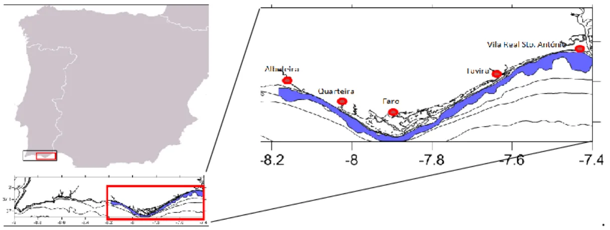
The South Portuguese coast is located in the SW limit of the Iberian Peninsula and the NW limit of the Gulf of Cadiz. The study area for this work is the South Portugal coast, from Albufeira to Vila Real de Santo António (Fig. 2.1). Here, the continental shelf is relatively narrow (8 km to 28 km) (Dias, 1987). Due to the southern wind’s dominant direction, the West part of the Algarve coast is called Barlavento (upwind) and the East side, Sotavento (downwind) (Magalhães, 2001) The coast of the Algarve is characterized by wave-regime less than 1 m wave height and by a less than 5 seconds mean period (Instituto Hidrográfico, 1994) and is a mesotidal type of coast with an average tidal range of 2 m (Moita, 1986; Bettencourt et al., 2004). The southern shelf is characterized by a relatively low energy hydrodynamic regime, with eastward current patterns imposed by the Atlantic flowing parallel to the shoreline with a speed less than 25 cm/s (Moita, 1986), and warmer water temperature than the western shelf (Fiúza, 1983).
Two main rivers discharge at the South Portuguese coast: the Arade and the Guadiana (the largest river in the study area). The Alqueva dam regulates over 80% of the freshwater flow in the Guadiana estuary since 2002, which decreases sedimentation in coastal waters and changes the mineral composition of the sediments transported (Caetano et al., 2006). The mean annual discharge of the Guadiana River is around 200 m3/s, influencing the adjacent coast waters up to 10km from the coast on heavy rainfall periods (Cravo et al., 2006). Under weak river discharges, the water characteristics of salinity, Chlorophyll a and nutrients are regulated by upwelling and relaxation regimes (Relvas and Barton, 2005).
The wind regime appears to be the major physical forcing affecting the oceanographic processes in the coast, predominantly northwesterlies, with an eastward component favourable to upwelling. This wind pattern explains the occurrence of waters with lower temperature and salinity in the coastal region and warmer and saltier water with characteristics typical of those found off the Gulf of Cadiz circulating offshore (Relvas and Barton, 2002). Other physical factors further than wind stress have influence on the
9 oceanographic processes and upwelling intensity, such as the coastline configuration and the morphology and bathymetry of the continental shelf (Oliveira et al., 2009). Among the water masses involved in the oceanic circulation dynamics in the Gulf of Cadiz, the Atlantic Surface Water and the Mediterranean Outflow Water are the main water masses that control the present-day sedimentary dynamics in the Algarve proximal margin (Ochoa & Bray, 1991). The study area is therefore influenced by the intersection of three Atlantic-Mediterranean bioregions - Mauritanian, western Mediterranean and Lusitanian region (Maldonado and Uriz, 1995).
. Fig. 2.1 - Study area.
2.2 Abundance data
Data on abundance was collected by IPMA, once a year in July, since 1986, along the Algarve. A data series from 1999 to 2011 was provided by IPMA for this work.
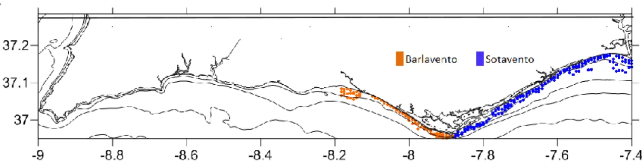
For the collection, two dredges are used simultaneously: a clam dredge (20-mm teeth) and a razor-clam dredge (35-mm teeth) both with a mouth opening of 64 cm. Sampling is carried out along 108 transects perpendicular to the coast with two to three samples taken at each transect, at different depths: (A) 3 m; (B) 4.8 m; (C) 6.6 m; (D) 8.4 m; (E) 10.2 m; (F) 12 m; (G) 13.8 m; (H) 15.6 m. Due to problematic areas West of Albufeira, study site was limited to this point (figure 2.2). Dredges were towed for 5 min at a mean speed of 2kn, sweeping an area of 144 m2. Counts from each dredge are individually kept in plastic bags and later in laboratory individuals are identified, measured and weighed.
10
.
Fig. 2.2- sampling stations in Barlavento and Sotavento.
2.3 Data treatment
Surfer biomass distribution maps
Codes for each species were created concatenating the first three letters of the genus and species: CHAGAL – C. gallina, DONTRU – D. trunculus, SPISOL – S. solida and ENSSIL – E. siliqua. The database was created using Microsoft Office Excel® and divided by species, by year, and by Sotavento/Barlavento region. It includes latitude, longitude, and abundance values.
Raw abundance values were transformed with the equation. Log10 (biomass + 1)
and this became the variable. The reason why this is done is to reduce error created by the large differences in abundance values.
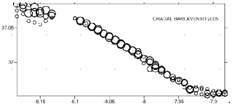
First we create Post Maps importing each database into Surfer, which represent the sampling points for each species/year by a marker. This marker was changed to be proportional to the sample, so we can visually see the relative abundance in each sampling station (figure 2.3).
Using the Post Map as a guide, it is possible to digitize a Shape File. In other words, we go around the outer limit of our markers one by one, creating a line that defines the area where the sampling takes place, corresponding to existing abundance inside that area (Figure 2.4).
Contour Maps were created using multivariate universal kriging. One by one, each year sampled for each species is gridded, importing the correspondent Microsoft Office
11 Excel® spreadsheet previously created. The kriging type chosen to produce the is “block”, with spacing of 0.001. After gridding the data, it is transformed with the option GRID MATH using the formula.
Max (a, 0).
this will remove the zeros from the file. Gridding will, by default, measure the co-variance between samples and their relative similarity. The kriging method used is an interpolation method, which will evaluate the similarities between samples, and group them together in categories (in a scale) visually distinguished the different levels, from low to high abundance, in each sample area.
Using the Shape File previously created, the Grid (our Surfer modified database) is then blanked, which means only the abundance values inside the Shape File are mapped. The contour maps are created using the blanked grid file, choosing the colour scale and the data intervals, for a more visual comparison of the biomass found in each location each year (fig. 2.3 – 2.4). Using multivariate kriging simplifies the spatial model estimation and produces maps from years with less obvious spatial dependency (Rufino et al., 2008).
.
Fig. 2.3- Example of a post map for Chamelea gallina abundance in Barlavento (2005). .
.
12
Fig. 2.4- Example of a shape file for Chamelea gallina abundance in Barlavento (2005).
Environmental variables
The environmental variables (sea surface temperature - SST, chlorophyll a concentration, wind index and precipitation) and data treatment are described below. Sea surface temperature (SST) - Monthly SST data (ºC) was retrieved online from the NASA MODIS-Terra 4km (11micron/day) satellite, form February 2000 to December 2010. Unfortunately, earlier data was not found (from Jan 1998 to Jan 2000). Coordinates for the sample area of Barlavento and Sotavento were used, so all the study area was covered. SST was correlated with 1 month, 2 months and 3 months prior to spawning, during spawning season, and 1 month after spawning season for each species (Refer to statistical analysis).
Chlorophyll a concentration - Monthly chlorophyll a concentration data (µg/l) was retrieved online from the NASA SeaWiFS 9km satellite, from January 1998 to December 2010, with coverage from all the study area of Barlavento and Sotavento. chlorophyll a data was used to study its influence both on the larval and the adult stages. Chlorophyll a concentrations (µg/l) were correlated with 1 month, 2 months and 3 months prior to spawning, during spawning season, and 1 month after spawning season for each species (Refer to statistical analysis).
Rainfall - Average monthly rain values (mm³) from January 1998 to December 2010 were collected from SNIRH (National System for Hydric Resources Information) from S. Brás de Alportel station 31J/01C (Sotavento). Daily rain fall (mm³) was summed for each month and this value was directly correlated with species abundance in the year after. Rainfall values were correlated with 1 month, 2 months and 3 months prior to spawning, during spawning season, and 1 month after spawning season for each species. Wind - Wind data was used from the Meteorological Service of Faro Airport (Sotavento), with daily records of average wind speed (m/s) and direction from January 1998 to December 2010. Data on wind direction (WD) was used to create a direction scale (D) from 1 to 8 according with the sector of the wind direction.
13 (D) was used to generate situation very favourable, unfavourable or moderately favourable with respect to larval dispersion (during spawning months). These conditions were defined differently for Sotavento (East) and Barlavento (West) of the Algarve coast. Very Favourable wind directions were assigned a value of 2, moderately favourable wind direction was assigned a value of 1, neutral wind was assigned 0, and unfavourable wind direction was assigned -2 (Fig. 2.5) .
.
Figure 2.5- wind index values: a) sector (D), b) wind direction (º), c) Barlavento wind value (very favourable (2), favourable (1), neutral (0), unfavourable (-2)), d) ) Sotavento wind value (very
favourable (2), favourable (1), neutral (0), unfavourable (-2)).
Average daily wind speed was transformed into the Beaufort scale. Wind indexes were created for the Barlavento and Sotavento coast by multiplying the dispersion by the Beaufort scale. Highly positive values of the wind index correspond to conditions highly favourable to larval dispersion while negative values are equivalent to wind that moves the larvae away from the coast. Monthly averages of the wind index were calculated. Wind speed was correlated with spawning season, and 1 month after spawning season, since in theory adults are sessile and only larvae may be affected by wind.
14
Statistical analysis
It was taken in consideration the theoretical influences of the different environmental parameters measures, in relation to the different life stages of each of the four bivalve species studied. All biomass indexes, measured every year in June, were correlated with the environmental parameters from the year before. Observed abundance values were compared with Surfer® abundance estimated values and only the observed values were used for all the statistical analysis (Annex 1).
Two linear regression models with annual abundance as a function of environmental variables were considered. The models were applied separately to the Barlavento and Sotavento regions:
1) Influence of the environmental conditions during the spawning season on the adult abundance of the following year.
ABUNDANCEt+1 = f (RAIN1t, RAIN2t, RAIN3t, CHLO1t, CHLO2t, CHLO3t, TEMP1t,
TEMP2t, TEMP3t).
where ABUNDANCE = biomass in year t+1; the environmental monthly variables precipitation (RAIN), chlorophyll a concentration (CHLO) and sea surface temperature (TEMP) were concatenated with the values 1, 2 and 3, indicating the first, second and third months of spawning, respectively. The spawning months were defined for each species based on previous maturity studies and are indicated in Table 2.1. The variable wind index (WIND) was not considered because in this model, the environment is considered to influence the condition of adults and therefore larval survival, and wind could only have an indirect effect by influencing primary production, a variable already considered in the model.
2) Influence of the environmental conditions during larval dispersion on the adult abundance of the following year.
In this case, the spawning period of each species plus one month was considered (Table 2.1), ranging from 3 months to E. siliqua to 6 months for D. trunculus.
15
ABUNDANCEt+1 = f (WIND1t, WIND2t, …., RAIN1t, RAIN2t, …., CHLO1t, CHLO2t, ….,
TEMP1t, TEMP2t, ….).
The environmental variables have the same meaning as before, and this time wind indexes (WIND) were considered.
The significance of the variables was evaluated fitting the models to the data with stepwise regression (PROC REG, SAS Institute Inc. 2008). Variables are evaluated twice, by the significance of the regression coefficient (p-value < 0.05) and by the significance of the same term when it enters the model last (Wald chi-square test). A nonsignificant Wald test (p-value > 0.05) results in the removal of this term from the model.
Correlation between abundance and environmental indexes were calculated with significance considered for p-values < 0.05.
Table 2.1- Spawning period of the studied species.
D J F M A M J J A S O N D M00 M01 M02 M03 M04 M05 M06 M07 M08 M09 M10 M11 M12
Spisula solida SPISOL
Donax trunculus DONTRU
Chamelea gallina CHAGAL
Ensis siliqua ENSSIL
3 months before spawning Spawning 1 month after spawning Sp.
CODE SPECIES
16
3 Results
3.1 Spatial distribution
Spisula solida presented higher biomass in 2003 both in Barlavento and Sotavento,
followed by 2004 and 2002. Lowest S. solida biomass was found in Barlavento in 2010 and in Sotavento in 2008. S. solida highest abundance is consistently found in the areas from Albufeira to Faro (Barlavento) and from Faro to Tavira (Sotavento). West of Tavira is where abundance was constantly relatively lower (fig. 3.1-3.2).
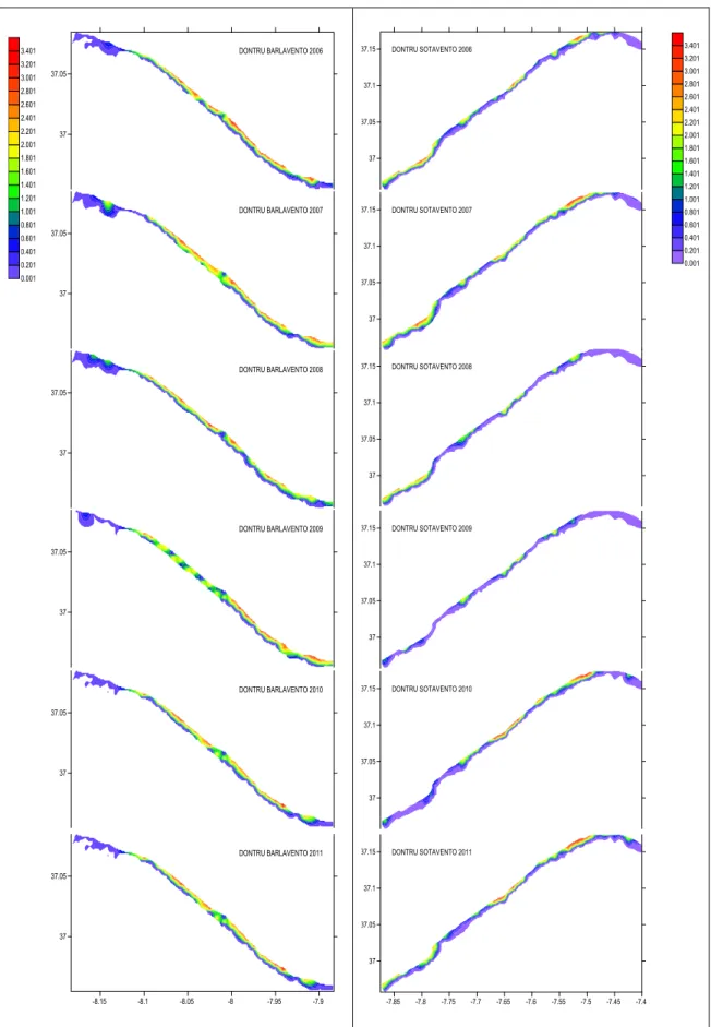
Donax trunculus showed lowest biomass both for Sotavento and Barlavento in 1999.
Highest biomass values were found in the year of 2003 both for Sotavento and Barlavento. Second highest year of abundance was 2001 in Barlavento and 2006 in Sotavento. D. trunculus is distributed along the study area, with exception of Albufeira and Vila Real de Sto. António, where abundances were consistently lower (fig. 3.3-3.4).
Chamellea gallina showed highest biomass in 2002 in Barlavento and in 2006 in
Sotavento. Lowest biomass in 2010 in Barlavento and in 2001 in Sotavento. C. gallina reaches higher abundance levels in the area of Vila real de Sto António, followed by Tavira. Some banks are found over the years in the region between Quarteira and Albufeira, and in some years in Albufeira (fig.3.5-3.6).
Ensis siliqua showed higher biomass values in 2005 for Barlavento and in 2004 for
Sotavento. Lowest biomass both for Barlavento and Sotavento in 2007.
E. siliqua shows preference for very shallow areas along the coast of Sotavento, with
some banks distributed along Olhão and Tavira mainly. In the Barlavento, distribution occurs along all depths (up to 15.8m) with higher abundances generally between Quarteira and Faro (fig. 3.7-3.8). This species abundance is relatively very low compared with the other 3 studied species, which reveals the overexploited banks are still recovering (unpublished data provided by Miguel Gaspar (IPMA) during the study). Overall, higher abundance occurred for all species between 2002 and 2006, and lowest abundance levels occurred in the years of 1999, 2001 and between 2007 and 2010.
17
18
Fig. 3.2 – S. solida spatial variation in Barlavento and Sotavento from 2006 to 2011.
19
20
21
22
23
24
25
3.2 Environmental variables
Monthly average SST was generally lower in the winter months - around 14ºC to 16ºC, between January and March, and especially low during the months of February. Minimum SST registered was 13.3ºC in February 2009. From March until May SST rises steadily (around 1ºC per month) and the greatest SST rise is clear between May and June (averages from 18ºC to 21ºC). Between June and August SST continues to rise steadily. Higher SST are recorded during summer months – around 20ºC to 23ºC between July and September, with higher SST value recorded in August 2010, 24.6ºC. There was no significant difference in temperature between the two parts of the South coast of Portugal (Barlavento and Sotavento) (fig. 3.9 and fig.3.10).
.
.
Fig. 3.9- Mean monthly SST variation in Barlavento between Jan 1998 and Dec 2010.
.
26 Monthly average chlorophyll a concentration levels vary along the year but are consistently higher between January and April in both regions. There is a clear distinction in chlorophyll a concentrations in Barlavento and Sotavento for the winter months. Between February and April, chlorophyll a concentrations in Barlavento average 2µg/L and higher, whereas in Sotavento average is around 1.3 µg/L. Highest chlorophyll a concentration was registered for Barlavento in January 2010, with 4.7µg/L. In May, chlorophyll a levels decrease on both sides of the coast, remaining relatively constant at 0.8µg/L – 1µg/L until October, where there is a slight increase to about 1.3µg/L in Barlavento and 1.1µg/L in Sotavento, decreasing back to around 1µg/L in December, on both sides on the coast. Lowest chlorophyll a concentration registered was 0.39µg/L in August 2005, in Sotavento (fig. 3.11 and fig. 3.12).
Fig. 3.11- Mean monthly chlorophyll a variation in Barlavento between Feb 2000 and Dec 2010.
27 Monthly average total precipitation was highest in December averaging 140mm³ and reaching a maximum of 392.2mm³ in December 2009. Total precipitation decreases from December until February, stabilizing trough to March (between 71 mm³ - 75 mm³). This pattern is seen again with total precipitation decreasing in April, and stabilizing through May. There is an accentuated decrease in total precipitation between May and June (average 43.6 mm³ and 9.8 mm³, respectively). July is the month with lowest average precipitation registered, followed by August and June. In September there is an abrupt increase on average precipitation, compared to August (from average 7.7 mm³ to 53. 6 mm³) and again from September to October where average monthly precipitation is 92 mm³. In November there is a decrease in precipitation (average 60.4 mm³) rising to its maximum in December (fig. 3.13).
.
. Fig. 3.13- Mean monthly precipitation between Jan 1998 and Dec 2010
Monthly average wind conditions are very distinct for Barlavento and Sotavento. This parameter shows the greatest monthly variation from our environmental parameters tested. In Barlavento, across most of the year, monthly average wind index is negative, in particular between September and April. Most favourable wind conditions occur in May and in July, with wind index close to 0 in June. The opposite conditions occur in the Sotavento; where across the whole year, monthly average wind index is above 0, with some annual variations. Still it is clear there is not a smooth increase or decrease in wind conditions across the year. In January, wind index is around 1, increasing in February to around 2, and decreasing steadily until May, the most unfavourable month for wind dispersal (wind index 0.75). Oscillations continue throughout the year with a
28 favourable peak in June, corresponding to the month with most favourable wind index, and an unfavourable peak in November, reaching values close to 0 (Fig. 2.14 – fig. 2.15).
.
.
Fig. 3.14- Mean monthly wind index variation in Barlavento between Jan 1998 and Dec 2010. .
.
Fig. 3.15- Mean monthly wind index variation in Sotavento between Jan 1998 and Dec 2010.
3.3 Statistical analysis
There were some significant findings using the Stepwise linear regression analysis for the two models tested (3 months before spawning – spawning + 1 month):
29 In relation to 3 months before spawning season, SST was positively correlated for S.
solida abundance both in Sotavento and Barlavento in December (3 months before
spawning period) (p-values = 0.0273 and p-value = 0.0144 respectively). For D.
trunculus, total precipitation was positively correlated with abundance in Barlavento in
December (3 months before Spawning) (p-value = 0.002). For C. gallina, total precipitation was positively correlated with abundance in Barlavento, in March (3 months before spawning) (p-value = 0.009). Chlorophyll a concentration was positively correlated with C. gallina in Barlavento in May (1 month before spawning) (p-value = 0.0023). E. siliqua showed no correlation with any environmental factors before spawning (Table 3.1).
Table 3.1- Statistical results for the model ‘3 months before spawning’ TEMP_BL_M00: mean SST for Barlavento in December, TEMP_ST_M00: mean SST for Sotavento in December, RAIN_M00:
mean precipitation in December, RAIN_M03: mean precipitation in March, CHLO_BL_M05: mean chlorophyll a concentration for Barlavento in May.
.
. In relation to the spawning season + 1 month after spawning, total precipitation was positively correlated with S. solida abundance relations both in Barlavento and Sotavento, in March (spawning season) (p-value = 0.0176 and p-value = 0.0178, respectively). Wind index was negatively correlated with S solida in Sotavento, in March (spawning season) (p-value = 0.0277). Total precipitation was negatively correlated with S. solida abundance in Sotavento, in June (1 month after spawning season) (p-value = 0.0187). Total precipitation was positively correlated with D.
trunculus abundance in Sotavento, in March (spawning season) (p-value = 0.0411).
Chlorophyll a concentration was negatively correlated with D. trunculus abundance in Sotavento, in March (p-value = 0.0241). Total precipitation was negatively correlated with C. gallina in Barlavento, in June (spawning season) (p-value = 0.0243). Both wind
variable p-value variable p-value
TEMP_BL_M00 0.015 1191.32 242.4 TEMP_ST_M00 0.0273 RAIN_M00 0.002 1.01 - - -RAIN_M03 0.009 0.73 - - -CHLO_BL_M05 0.002 146.95 - - -Parameter estimate Sotavento Barlavento
30 index and chlorophyll a concentration were positively correlated with C. gallina abundance in Barlavento, in August (spawning season) (p-value = 0.0037 and p-value = 0.0093, respectively). Chlorophyll a concentrations were positively correlated with C.
gallina abundance in Barlavento, in September (1 month after spawning) (p-value =
0.093). Wind index was positively correlated with E. siliqua abundance in Sotavento, in April, corresponding to spawning season (p-value 0.036) (Table 3.2).
Table 3.2- Statistical results for the model ‘spawning + 1 month’. RAIN_M03: mean precipitation in March, WD_ST_M05: wind index for Sotavento in May, RAIN_M06: mean precipitation in
June, RAIN_M03: mean precipitation in March, CHLO_ST_M03: mean chlorophyll a concentration for Sotavento in March, RAIN_M08: mean precipitation in August, WD_BL_M06:
wind index for Barlavento in June, CHLO_BL_M08: mean chlorophyll a concentration for Barlavento in August, CHLO_BL_M09: mean chlorophyll a concentration for Barlavento in
September, WD_ST_M04: wind index for Sotavento in April.
.
variable p-value variable p-value
RAIN_M03 0.02 9.95 2.88 RAIN_M03 0.018 - - - -175.5 WD_ST_M05 0.023 - - - -3.97 RAIN_M06 0.019 - - - 29.25 RAIN_M03 0.041 - - - -19.13 CHLO_ST_M03 0.024 RAIN_M08 0.02 -3.13 - - -WD_BL_M06 <0.001 108.18 - - -CHLO_BL_M08 0.035 78.1 - - -CHLO_BL_M09 0.001 39.14 - - -ENSSIL - - - 29.25 WD_ST_M04 0.036 Sotavento Parameter estimate spawning + 1 month Barlavento CHAGAL Species code DONTRU SPISOL
31 The significant variables identified with the linear model, were associated with the life cycle period, in table 3.3.
Table 3.3- Statistical results showing the significant variables (R: precipitation levels (mm³), C: chlorophyll a concentration (µg/l), T: SST (ºC), W: wind index) for a) Barlavento and b) Sotavento.
(+): positive correlation (-): negative correlation.
a) Barlavento
D J F M A M J J A S O N D M00 M01 M02 M03 M04 M05 M06 M07 M08 M09 M10 M11 M12
Spisula solida SPISOL T (+) R (+)
Donax trunculus DONTRU R (+)
Chamelea gallina CHAGAL R (+) C (+) W (+) R (-) C (+)
C (+)
Ensis siliqua ENSSIL
b) Sotavento
D J F M A M J J A S O N D M00 M01 M02 M03 M04 M05 M06 M07 M08 M09 M10 M11 M12
Spisula solida SPISOL T (+) R(+) W(-) R (-)
Donax trunculus DONTRU R(+)
C (-)
Chamelea gallina CHAGAL
Ensis siliqua ENSSIL W(+)
3 months before spawning Spawning 1 month after spawning SPECIES Sp.
CODE
SPECIES Sp. CODE
32
4 Discussion
4.1 Species spatial distribution
In the present study bivalve abundance variation between 1999 and 2011, across a very fine spatial grid of 0.8 km in the fishable areas, was mapped and described. The spatial distribution maps revealed S. solida had higher abundance in the Barlavento region. Martins et al. (2012) describe a muddy patch developed off the Guadiana estuarine system, which provides most of the sediment supply to the South coast of Portugal. These sediments do not favour S. solida settlement and this may explain the low abundances in the Sotavento (closer to the Guadiana estuary). The year 2010 shows a high decrease in the abundance of this species, which can be attributed to the harsh winter experienced in 2009, in which strong winds and consequent wave action may have disturbed the populations in the sediment. C. gallina shows the same abrupt reduction in stock size for 2010, but the result is not consistent for the other two species, whose abundance was maintained. C. gallina shows higher abundance in Sotavento region, especially by Vila Real de Sto. António, which may be the result of preference for finer sediment and strong freshwater inputs and food supply from the river Guadiana. D. trunculus and E. siliqua show similar distribution to S. solida, with lower abundances close to Vila Real de Sto. António but, unlike S. solida, they also show low abundance in the Albufeira.
One very important factor to take in consideration is fishing pressure, which may affect species distribution and survival in a different way, and was not considered in this work, because the landings are more or less constant, defined by daily quotas and fishing seasons, therefore not showing significant fluctuations.
Dolbeth et al., (2006) study, in the Algarve coast, concluded S. solida’s distribution appeared to be influenced by the cross-shore sediment dynamics, a seasonal phenomenon, suggesting that sediment dynamics may have a positive or a negative correlation with species abundance, depending on environmental conditions.
In the timeframe between 1999 and 2011, S. solida and D. trunculus show the highest abundance in the year of 2003. E. siliqua showed higher abundance in 2004 (Sotavento) and 2005 (Barlavento), C. gallina showed the highest abundance in 2002 (Barlavento)
33 and 2006 (Sotavento). Dolbeth et al., (2006) as mention that, in the year 2001, the absence of S. solida’s adults was caused by overfishing. We may infer, in agreement with Defeo (1996), that extremely low abundances will result in higher recruitment, which could explain the higher S. solida abundance in 2003. On the other hand, the severe winter in 2009, with strong winds and stormy conditions, may have washed part of the population to an area of less favourable conditions, reflecting the low general abundance of the bivalve species in 2010 (M. Gaspar, personal communication).
Spatial analysis can be used to establish priority conservation areas for management purposes, and to analyse the persistency of regional diversity patterns. (Rufino et al., 2008). It is clear for our results for the E. siliqua population, that recovery is far from accomplished, with much lower abundance for this species than for the other three species studied. Overall, distribution maps provide an easy and intuitive picture of the population’s abundance variation, both in space and time, and may be a helpful tool for fisheries management.
4.2 Influence of environmental parameters
Spisula solida
The most significant variable correlated with S. Solida abundance was Sea surface temperature (SST) positively correlated in December (three months before spawning) in all the coast (Barlavento and Sotavento). Temperature has been considered as an important parameter in determining bivalve reproductive development and spawning (Gribben, 2005). Chícharo & Chícharo (2001) suggest small variations in water temperature can cause shifts in their reproductive cycle. The monthly average SST results in this work showed no significant differences for this environmental parameter in different regions (Barlavento and Sotavento). Results suggest an increase in SST during gametogenesis; will benefit S. solida abundance in the following year in all South Portugal’s coast.
The second significant variable is the level of precipitation in March, during the spawning season for S. solida, also positively correlated with abundance in the following year (both in Barlavento and Sotavento), therefore we may assume the increase of freshwater input will contribute for population growth and extends all along
34 the coast, including the west end of the species distribution. Precipitation levels in June were negatively correlated with S. solida abundance, but only in Sotavento. The month of June corresponds to the period when most individuals are spent and larvae are settling (Martins et al., 2012). High precipitation levels during this month will affect mostly the Sotavento coast, suggesting that early life stages on the eastern side of the coast are more sensitive to salinity variations, due to its closer proximity to the Guadiana River. Baptista & Leitão (2014) suggested, in their recent study of S. solida populations in the same study area, that winter river discharges during the summer negatively affected S. solida catches on the South coast, which goes in conformity with our results.
The Wind Index in May, showed a negative correlation to S. solida abundance. May is the middle of the spawning season, suggesting that the wind has a significant influence on larvae dispersal and settlement, thus in recruitment. The average monthly wind indexes, elaborated in this study, showed that May was generally the month with the most unfavourable influence on larval dispersal across the year, for the Sotavento region. The results obtained in this study support the hypothesis that larval dispersal is favoured by wind conditions and that wind is crucial for this species distribution and abundance.
Donax trunculus
Precipitation was the most important variable associated with D. trunculus abundance. Significant precipitation was associated with the months of December and March from the year previous to abundance estimation. Precipitation in December (3 months before spawning), positively affected the Barlavento populations. During this period, the adult populations are undergoing gametogenesis and may benefit from the additional nutrient load and freshwater input associated with periods of heavy rain. The influence of rain on the Barlavento in associated with a month of heavy rain, when the freshwater influx form the Guadiana, rich in nutrients, is able to reach the most western populations (Cravo et al., 2006). Precipitation in March (spawning season) was positively correlated with D. trunculus abundance in Sotavento. We suggest that, similarly to what was observed for S. solida, the precipitation in March, contributes with higher nutrient input for the larval and juvenile stages.
35 The Sotavento populations are also negatively influenced by Chlorophyll a concentration during March, that is, abundance is favoured by low concentrations, likely associated with downwelling, a situation that tends to keep larvae inshore and cause high-settlement rates (Shanks and Brink, 2005).
Chamelea gallina
Precipitation in March (3 months before spawning) was positively correlated with the abundance of C. gallina in Barlavento. The same result has been noticed for S. solida in Barlavento. We may infer that several species may be affected by precipitation levels, with winter months of heavy rain favouring the abundance of S. solida and C. gallina the year after.
Chlorophyll a concentrations in May (1 month before spawning season), are positively correlated with C. gallina abundances in Barlavento. High quality and quantity of nutrients and freshwater input to the adult populations may significantly contribute to higher egg quality (Utting & Millican, 1997), and reproductive success. Gaspar et al. (2004) suggest C. gallina individuals, born at the beginning of the spawning season, may benefit from rapid growth during summer, while the ones born later will benefit from these conditions for only a short period of time. The same environmental conditions that promote growth rates and egg quality may also result in earlier spawning and improved larval survival (Gaspar et al. 2004).
Chlorophyll a concentrations both in August and September (spawning season) were also significant, but this time positively correlated with C. gallina abundance in Barlavento. Several studies have reported that the reproductive cycle of C. gallina was significantly by food availability; Ojea et al., 2004; Albentosa et al., 2007). This result corroborates once more the importance of chlorophyll a concentration both for adult reproduction and for larval growth and survival, assuming the higher nutrient, higher freshwater input from the river mouth is implicit with higher chlorophyll a concentrations
Precipitation levels in August (spawning season) were negatively correlated with C.
gallina abundances the following year in Barlavento. August was shown to be the
36 Previous discussion suggested the bivalve populations of S. solida in Barlavento (further from Guadiana river mouth) may be more sensitive to freshwater inputs. Again this may be the case, which corroborates the previous assumption. Spatial distribution maps for this species showed higher abundance in Sotavento by Vila Real de Sto. António, the closest area to the river Guadiana estuary and in Barlavento between Albufeira and Quarteira. Both regions are very different in terms of nutrient load, freshwater input and sediment type. This reinforces the suggestion that populations living on both sides of the coast are adapted to very different environmental conditions. Wind index in June (spawning season) was positively correlated with C. gallina abundance in Barlavento. The analysis of wind patterns (3.14) shows that the wind index is positive during the months of May to July and that June, in the middle of this period, shows lower values. The shift in the June wind index may be important for larval dispersal and survival. C. gallina distribution is the widest from the studied species, 4m to 24m; therefore it is possible that the wind is a crucial factor for the dispersion and survival of this species.
Ensis siliqua
This species shows the lowest abundance levels from all the species studied, what may have resulted in poor correlations with environmental variables studies, just due to poor sampling. Despite this, there was a positive correlation between the abundance of E.
siliqua and wind index in April (spawning season) for Sotavento. Once again, results
suggest larval dispersal may be determinant factor for adult abundance.
Globally, the two most important significant variables were chlorophyll a concentration and precipitation. Chlorophyll a is important from late spring to early fall, affecting mostly the Barlavento populations. The influence is associated mostly with the post-spawning periods, affecting the abundance in the following year. In one case (C.
gallina), chlorophyll affected late pre-spawning stages. On the Sotavento, primary
production does not have such a great influence, likely because these populations are closer to the main nutrient source (the Guadiana River) and may have a steadier supply throughout the year. The exception is D. trunculus, negatively affected by chlorophyll a in early spawning, what may be a result of associated wind patterns adverse to larval