Economic centrality : how much is economics and how much is geography?

Nuno Crespo, M. Paula Fontoura, & Nádia Simões

Economic Centrality: How Much is Economics and How

Much is Geography?

W

P

Economic Centrality:

How Much is Economics and How Much is Geography?

(a) * _{Nuno Crespo,} (b) _{M. Paula Fontoura, and} (a)_{Nadia Simoes}

(a) _{Instituto Universitário de Lisboa (ISCTE – IUL), ISCTE Business School Economics}

Department, BRU – IUL (Business Research Unit), Lisboa, Portugal.

(b) _{Instituto Superior de Economia e Gestão (ISEG – Universidadede Lisboa), UECE}

(Research Unit on Complexity and Economics), Lisboa, Portugal.

* Author for correspondence. Av. das Forças Armadas, 1649-026 Lisboa, Portugal. E-mail: nuno.crespo@iscte.pt.

Abstract: Proximity to the markets is a key determinant of the location of firms because distance still matters, as recently reported in the literature. In this paper, based on an adapted version of the most standard centrality index we propose a decomposition method which allows isolating the influence of: (i) internal and external factors; (ii) economic and geographical aspects. In order to illustrate our methodology, we consider data for 171 countries. This empirical example leads to the conclusion that the centrality level of the countries derives from different sources, requiring therefore different policy interventions in order to improve it.

Keywords: centrality, peripherality, economic geography, distance. JEL Codes: F14; F68; R30.

Acknowledgements

The authors are grateful to the Fundação para a Ciência e para a Tecnologia (PEst-OE/EGE/UI0315/2011 and PEsa-OE/EGE/UI0436/2011) for financial support. The usual disclaimer applies.

Economic Centrality:

How Much is Economics and How Much is Geography?

1. Introduction

Globalization is one of the most remarkable trends of the last decades (Head and Mayer, 2013) with trade growing faster than GDP since 1980 (Berthelon and Freund, 2008). Is this equivalent to say that the friction of distance is not so important now as it was in the past? Recent empirical studies on this topic provide a clear negative answer to this question. Rather, as shown by Disdier and Head (2008), the influence of distance on trade is consistently high since the middle of the last century. The average result emerging from their meta-analysis points to the fact that a 10% increase in distance has a negative impact of 9% on bilateral trade. In this context, the advantage of centrality (or the penalization of peripherality) is obvious and can be grounded on at least four main reasons.

First, firms want to locate where the markets are. In fact, proximity to the markets is one of the location determinants traditionally included in the empirical studies. However, in most cases, only the demand that is specific to the region/country under analysis is considered, i.e., the importance of neighbouring spaces is ignored (Head and Mayer, 2004). On the contrary, the concept of centrality explicitly incorporates and quantifies the external influence.

Second, also at the theoretical level, the importance of the proximity to the markets is for long considered by the location theory. Since the beginning of the 1990’s, the new economic geography approach brings this kind of considerations to the mainstream economics, discussing alternative mechanisms through which agglomeration may occur. In this group of models the location of production depends on the relative strength of centrifugal and centripetal forces. Increasing returns and decreasing trade costs are key elements that generate an uneven spatial distribution of economic activity (Fujita et al., 1999). This perspective highlights therefore that, behind first nature aspects, also second nature dimensions matter for final location configurations. As stated by Krugman (1993, p. 131), “firms that have an incentive to concentrate production at a limited number of

locations prefer, other things equal, to choose locations with good access to markets; but access to markets will be good precisely where a large number of firms choose to locate”. Trade costs also play an important role in the heterogeneous firms models. In this context, the reduction of trade costs will force the least productive firms to exit and will generate a reallocation of market shares from less productive to more productive firms (Melitz, 2003).

Third, the centrality theme has extremely important implications for economic policy, namely in the areas of transports and economic and social cohesion (Ottaviano, 2008). In fact, the centrality of the spaces depends critically on accessibility and, as Spiekermann and Neubauer (2002, p. 7) affirm, “accessibility is the main ‘product’ of a transport system. It determines the locational advantage of an area (…). Indicators of accessibility measure the benefits that the households and the firms in an area enjoy from the existence and use of the transport infrastructure relevant for their area”. Different interventions can be requested in order to minimize the disadvantage associated with peripherality. Therefore, a clear understanding of the factors that constitute an obstacle to an easier access to the markets is valuable knowledge for policy actors.

Fourth, economic centrality has been the subject of an intense debate not only due to the negative impact of remoteness from the markets but also to the positive relationship between centrality and per capita income (Redding and Venables, 2004).1

Given the importance of the centrality concept, it is not surprising the emergence of a broad range of measures aiming its empirical materialization. This group of indicators has its origin in the pioneering contributions by Keeble et al. (1982, 1988) and include, among others, the indexes suggested by Gutiérrez and Urbano (1996), Linneker (1996), Copus (1999), or Schürmann and Talaat (2000) (for a discussion of some of these measures see Spiekermann and Neubauer, 2002).

These centrality measures differ in their methodological options. However, a common shortcoming is the fact that they do not allow for identifying the relative contribution of geographical and economic components to the overall level of centrality. The present study addresses this specific issue by proposing an adaptation of the most commonly used centrality index and, based on that, a simple decomposition method that allow to identify the contribution of economics and geography both at internal and external levels.

1 _{Crespo and Fontoura (2006) confirm this causal link at regional level using data from Portugal.} Additionally, Redding and Schott (2003) establish a theoretical relationship between centrality and education attainment, reinforcing the advantage of a central position in terms of economic development.

The remainder of the paper is structured as follows. Section 2 presents the index and the decomposition method that we propose. Section 3 provides an empirical example of the methodology proposed. Section 4 presents some final remarks.

2. Decomposing Centrality

As we discussed in the Introduction, from the literature on economic centrality/peripherality several measures have emerged. The most commonly used index was proposed by Keeble et al. (1982, 1988). Using for the country under analysis and

for other countries, the index can be expressed as:

∑ (1)

where is a mass variable for country and the distance from to . Taking this index as inspiration we propose a new centrality measure:

∑ , (2)

where and are the shares of countries and in the total value of the mass variable taken as reference, and is the internal distance of country .

Equation (2) makes clear that the level of centrality exhibited by country depends on four dimensions, covering geographical and economic aspects both at internal and external levels. However, it does not allow us to identify how much each component contributes to the global score of the country. Before the discussion of this topic, we consider five methodological options necessary to calculate .

The first aspect regards the distance function considered. Despite the existence of other formulations and significant study on this issue, the use of a linear function is the simplest

and the most common choice. The second question is how to evaluate inter-country distances. Several options are available including great circle distances, distances by road, time distances, or transport costs. Of course, the choice is strongly conditioned by the availability of the data. The third aspect to be taken into account also concerns the measurement of the distance between countries and it is related to what location should be considered as reference? Two options are commonly used: a dimensional criterion (population, economic activity) or an institutional criterion. However, usually the two possibilities do not imply significantly different results. Fourth, what variable should be used to capture the economic dimension of the countries? GDP, population, employment, or some other variable related to the distribution of economic activity are among the most common choices.

The question that has been submitted to more intense debate, namely in the context of the so-called “border effect” literature, is the one concerned with the measurement of the internal distance (Anderson and van Wincoop, 2003). Following the proposal of Head and Mayer (2002), we can consider three types of measures (for a discussion on the influence of considering different measures see Chen, 2004). The first group of measures was suggested by Wolf (1997, 2000) and associate to a proportion ( ) of the distance to neighborhood countries. Wolf (2000) considers only the distance to the closest country and assumes 0.25. In turn, Wolf (1997) considers 0.5 and calculates the average distance from the countries with a common frontier. The second type of measures is supported on infra-national distance measures, i.e., in the distribution of economic activity inside the national space. In general terms, these indicators require a much more demanding set of information for their construction. An exception is Wolf (1997) who considers only the distance between the two largest cities of the country. Alternatively, Wolf (2000) proposes to multiply that distance by the double of the weight of the second largest city on the sum of the two cities. Chen (2004) uses the weighted average of the geographical distance between the major cities considering regional GDP’s as weights. The indicators suggested by Head and Mayer (2000) and Helliwell and Verdier (2001) can also be classified in this group but are more complex. For example, in the measure proposed by Helliwell and Verdier (2001), the internal distance is expressed as the “weighted average of intra-city distances, intercity distances, the average distance between cities and rural areas, and the average distance from one rural area to another” (Helliwell and Verdier, 2001, p. 1026). The third group of indicators associates the

internal distance with the area of the country, being therefore easy to calculate. Representing the area of country as , Nitsch (2000) and Melitz (2007) consider the radius of a hypothetical disk, i.e., . Other studies follow alternative ways. For example, Keeble et al. (1982, 1988) and Brülhart (2001, 2006) multiply the previous expression by while Head and Mayer (2000) and Redding and Venables (2004) multiply by , aiming to obtain “the average distance between two points in a circular country” (Redding and Vanables, 2004, p. 62).

The next step in our discussion (and the main contribution of the study) is to propose a simple method to decompose the global index into four parcels with specific interpretation. This is obtained as follows:

∑ ∑ (3)

where is the average internal distance ∑ and the total number of countries. The internal geographical component C1 assumes an equal distribution of the economic activity (i.e., each country capturing a fraction of total economic activity). Thus, the values obtained by each country only depend (negatively) on its geographical dimension, evaluated through its area, as commonly done in this type of measures. If the same portion of economic activity is located in a smaller country then we will say that this country is more central than another one with a larger dimension, where the economic activity is more dispersed in space.

In turn, the internal economic component is measured through C2 , being C2.1 a pure

internal economic component and C2.2 a geographical adjustment factor. C2.1

assumes a positive value when an above-average share of economic activity is located in that country, indicating that its centrality level benefits from a favorable position in economic terms. A negative value occurs when the country captures a below-average fraction of economic activity. Given that we fixed the internal distance at its average, the

differences between countries are fully attributable to this economic effect. Regarding C2.2 , it registers a value above 1 when the country is (geographically) smaller than the average and below 1 in the opposite case. The global effect C2 captures the internal economic component adjusted by the dimension of the country.

The centrality level of a given country depends not only of what happens at the internal level (the aspects analyzed so far) but also of external dimensions.

The external geographical component - C3 - is at the heart of the centrality concept. It assumes, once again, as in C1 , the equal distribution of economic activity in space and analyzes how far country is from the remaining countries. More remote countries suffer from a “tyranny of distance” (Battersby and Ewing, 2005), an expression, inspired by the tittle of the Geoffrey Blainey’s (1983) book, that became popular to summarize the idea that a negative position in this aspect is difficult to minimize and impossible to overcome in its full extension.

Finally, we should also consider the distribution of economic activity by the other countries. In this case, however, it is important to note that, by opposition to the preceding components, we cannot isolate a pure external economic component. The reason for that is straightforward. Obviously, the share of economic activity located outside is 1 but this does not give us any new insight. What really matters is the spatial distribution of that part of the total economic activity and, more specifically, its closeness to . Therefore, C4 is influenced both by economic and geographical aspects, assuming a positive value when economic advantages are obtained by countries closer to . Its minimum value is reached, for , when all the economic activity is concentrated in the farthest country.

One of the most important insights allowed by this decomposition methodology is that it offers guidance for policy interventions aiming to improve the centrality level of a country. Effectively, distinct policy measures can be recommended depending on the main weaknesses detected. Let us consider then each specific component. The improvement on the internal geographical component C1 can be obtained through better infrastructures, allowing a reduction on transport costs and times. In turn, if a country shows a low score on the internal economic component C2 , interventions should be devoted to the attraction of more economic activity to the country, for instance through

favorable conditions to FDI. For its part, rapid access to external countries is vital to improve centrality through component C3 . The creation and/or improvement of infrastructures that connect the country to foreign countries are adequate interventions to improve centrality. Component C4 is the only one that is out of control of national authorities. It depends on the distribution of economic activity across the remaining countries, an aspect that national policymakers do not influence in a direct way. Nevertheless, an indirect aspect may contribute to improve this component, namely the formation of regional integration blocks, with the elimination (or, at least, reduction) of trade barriers between the members of the block. This may attract more economic activity for the whole block, which is commonly composed by adjacent countries.

Until now we presented a simple procedure to identify the components that contribute to the level of economic centrality of each country. An obvious shortcoming of the method presented is nevertheless the fact that considering the equal distribution of economic activity across all countries as reference is not a realistic assumption since the countries differ substantially in spatial terms. In fact, an equal distribution presupposes that a country as small as Luxembourg should locate the same share of economic activity as a much larger country as China. This can only be accepted as a first approximation. In order to overcome this problem, we suggest an adjustment to the baseline decomposition method in which, instead of using as reference, we consider the share of each country in spatial terms. This can be seen as a topographic adaptation, somewhat in line with the approach followed by Brülhart and Traeger (2005) to measure the level of specialization. This new version can be therefore expressed as:

∑ ∑ (4)

in which and are the shares of the internal distances of and in the sum of all the internal distances, respectively.

Component C5 is similar to C1 in equation (3) but instead of we assume as reference the share of in terms of its internal distance ( ), which means that we are using internal

distance as a proxy for area. Considering C6 , we can verify that, in C6.1 , the countries are ranked according with the excess they exhibit vis-à-vis their share in spatial terms. A positive value is thus obtained when the country captures a higher proportion of economic activity than that it has in terms of area. The interpretation of C7 is also different from C3 in equation (3). Now, the distances to the remaining countries are not equally weighted. Instead, each destination country is weighted by . Finally, C8 evaluates the geographical adjusted external economic effect. This component assumes a positive value if the countries closer to have a higher share of economic activity than they have in spatial terms.

3. An Empirical Example

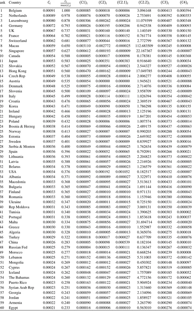
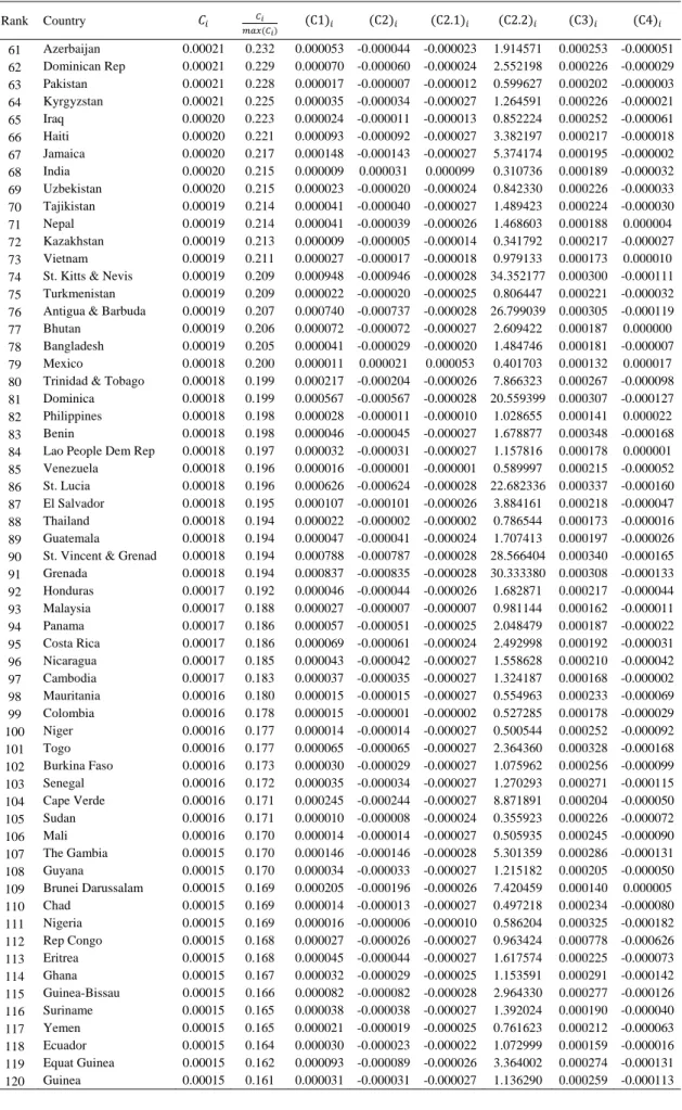
In order to illustrate the method discussed in the previous section, we calculate the centrality level for a group of 171 countries. Using data from World Bank, we consider information on GDP for 2011. Internal and external distances are obtained from CEPII. Thus, the following methodological options are considered: (i) geodesic distances; (ii) external distances between the largest cities; (iii) internal distances calculated as (Mayer and Zignago, 2011). Table 1 shows the aggregate centrality index ( ) for each of these countries.

[Insert Table 1 here]

Let us retain four main results from this evidence. First, there is an accentuated difference between the centrality levels of the most central countries and the remaining ones. In fact, only the sixth first countries exhibit a centrality index above 70% of the maximum value (Belgium). Second, in aggregate terms, it is evident a much central position of the countries of the north hemisphere. Third, Europe clearly shows the most favorable situation in what regards proximity to the markets, with seven countries in the best 10

(and 24 in the best 30) of the index. Fourth, Africa and Oceania show the worst positions in terms of centrality, being penalized in their capacity to reach the markets. The next step of our empirical example is to decompose the aggregate index aiming to verify the sources of centrality/peripherality in each specific case. The evidence is also shown in Table 1. Several interesting conclusions can be highlighted. The central idea to keep in mind is the fact that a high/low centrality level can be the derived from very distinct sources. Regarding component C1 we verify, obviously, that the smallest countries register the highest values, meaning that the same amount of economic activity located in a more confined space corresponds to a better access to that economic activity and therefore a higher level of centrality. A second and very important source of centrality is the internal economic component. Considering, more specifically, the component

C2.1 we verify that the countries with the highest scores are, in this order: USA, China, Japan, Germany, France, UK, and Brazil. This group contains some of the most powerful economic countries, all of them members of the G20. As we emphasize above, component C3 is critical to understand the concept of centrality, indicating the proximity to all the other countries. This proximity has an exclusive geographic dimension. The five countries that benefit the most from their location are from Africa (Republic of Congo and Democratic Republic of Congo) and Europe (Slovakia, Austria, Croatia, and Hungary). Finally, component C4 corresponds to the external economic component representing the degree by which a significant amount of economic activity locates close to the country under study. In this regard, Belgium, Canada, Netherlands, Luxembourg, and Korea constitute the group at the top of the classification.

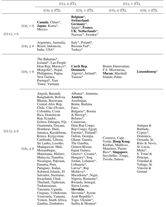
The best way to make clear the crucial idea that the sources of centrality are very different is by providing a classification of the different countries according to the specific combination they show in the main components that contribute to their centrality score. Four criteria are used, leading to a total of 16 possible combinations:

(i) C1 above or below average C1 . The case of C1 C1 occurs for the smallest countries, while C1 C1 for the largest countries.

(ii) C2.1 with a positive or negative value. C2.1 0 occurs when the country capture a proportion of total GDP above that associated with an equal distribution by all countries. In the opposite case, C2.1 takes a negative value.

(iii) C3 above or below average C3 . C3 C3 occurs in the case of the countries that benefit the most from their geographical position, i.e., that, in a pure geographical sense, are closer to the markets. Countries that locate far away from the markets have C3 C3 .

(iv) C4 with a positive or negative value. C4 0 occurs if there is a concentration of economic activity in countries close to the country under consideration. C4 0 corresponds to the case in which the largest part of economic activity is located far from the country considered.

Additionally, in order to establish the association between and the four components mentioned, the names of the countries are presented:

(i) In bold and with an * if 0.75 (see Table 1); (ii) In bold if 0.50 0.75;

(iii) With an * if 0.25

0.50;

(iv) Without any specific mention in the remaining cases. The results from this exercise are presented in Table 2.

[Insert Table 2 here]

While Table 3 explores in a qualitative way the results emerging from the decomposition method discussed, a quantitative analysis is also important, aiming to provide a more comprehensive perspective on the centrality sources. That analysis was already initiated in Table 1 but we can now move forward, exploring those results further (Table 3).

[Insert Table 3 here]

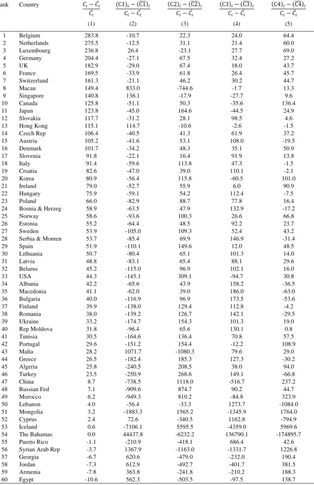
The column (1) of Table 3 compares the centrality level of each country with the mean value in relative terms. The first four countries exhibit a centrality level above 200% of

the mean of the 171 countries. Belgium and Netherlands – the two countries at the top of the ranking – have values corresponding to 283.8% and 275.5% above the mean of . The results also show that the first 16 countries in the centrality ranking present a value that exceeds the mean in more than 100%. The case of Bahamas, 54th _{of the ranking}

corresponds exactly to the mean while 117 countries have with a negative gap vis-à-vis ̅ .

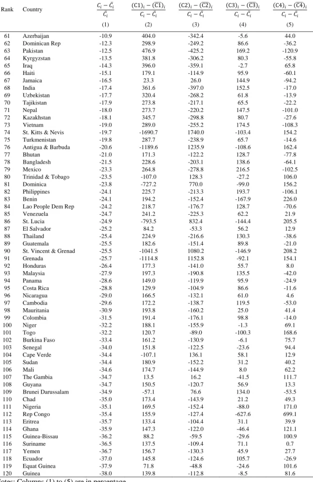
How much of the differentials in the centrality index should be attributed to the differentials founded in each specific component? The answer to this question is provided in columns (2) to (5) of Table 3. Let us consider the case of Luxembourg (ranked 3rd as regards ) as example. The positive gap from the average revealed by this country is due to its favorable situation in C1 , C3 , and C4 . The first is explained by its small dimension in geographical terms, the case of C3 by its central position regarding the remaining countries, namely its proximity to several markets of central Europe and the case of C4 by the fact that some economically important countries are located close to Luxembourg. The advantage in C4 is the most relevant in the explanation of the overall performance of the country in terms of centrality, accounting for 69.0% of the gap. On the negative side, Luxembourg shows an insufficient result regarding the internal economic component C2 . Looking for the results in a broader perspective, we can easily infer the strong heterogeneity among the distinct countries in what concerns the components that contribute the most for their centrality score.

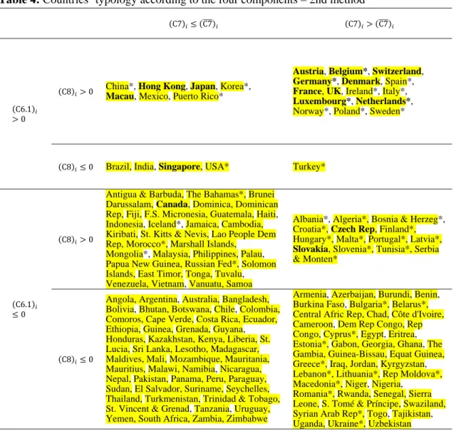
The empirical analysis conducted so far only considered the decomposition that assumes as reference an equal distribution by all countries. However, as we discussed in section 2, it is interesting to contrast the results from this case with the ones emerging from an analysis in which the spatial dimension of each country is taken as reference. This analysis was also developed in this study, following equation (4). The full range of results cannot be presented here due to space restrains but the classification of the countries according with criteria similar to those above discussed (with the necessary adaptation in terms of interpretation) is presented in Table 4.2

[Insert Table 4 here]

In this case, we only consider three components, namely C6.1 , C7 , and C8 . Regarding the classification according with , we follow the procedure already used in Table 2. Of course, the results show significant differences when compared with the first decomposition method above reported. This derives directly from the concept inherent to each one of the decomposition methods proposed in this study (equations (3) and (4)), reinforcing the advantage of their joint consideration.

4. Final Remarks

Based on an adjusted version of a standard index of economic centrality, the main contribution of this paper was the proposal of a decomposition method that allows to retain the influence of: (i) factors that are internal or external to the country under study; (ii) economic and geographic aspects. This is an important issue because very different policy interventions can be executed in order to overcome each specific weakness. Behind the methodological contribution, we provide an empirical illustration considering data for 171 countries. This empirical analysis makes clear that the roots of the centrality level of each country are very different, with positive and negative impacts of both economic and geographical factors. The final centrality score is therefore the net effect of a complex range of causes.

Based on the methodology discussed in this paper, several research avenues can be traced. First, it is important, of course, to extend the empirical exercise in order to improve our knowledge about the level and the sources of economic centrality of the countries. In this context, the analysis over a long-term period is certainly a fruitful way aiming to capture the main historical trends. Second, the existence of studies conducted at regional level for some countries is also useful to deepen our understanding of the phenomenon. Third, some methodological improvements can also be emphasized for future research. Especially important, in our perspective, is the possibility to adjust the decomposition method proposed in this study in order to capture the concept of sectoral centrality. In fact, we may argue that the level of centrality may be very different across sectors,

pointing to the interest of obtaining the centrality level of country i in each sector and studying the correspondent determinants. Still at the sectoral level, we can also conceive an extension of the decomposition method that associate centrality not only with the spatial distribution of the sector but also with the distribution of vertically-linked sectors. Finally, the empirical analysis conducted in the present study should be understood as a preliminary exercise. Its development aimed essentially an illustrative purpose but several refinements (for example regarding the methodological options on the measurement of distance) are welcomed.

References

Anderson, J. and van Wincoop, E. (2003), “Gravity with gravitas: A solution to the border puzzle”, American Economic Review, 93(1), 170-192.

Battersby, B. and Ewing, R. (2005), “International trade performance: The gravity of Australia’s remoteness”, Treasury Working Paper No. 2005-03.

Berthelon, M. and Freund, C. (2008), “On the conservation of distance in international trade”, Journal of International Economics, 75(2), 310-320.

Blainey, G. (1983), The tyranny of distance: How distance shaped Australia’s history, Pan-Macmillan.

Brülhart, M. (2001), “Evolving geographical concentration of European manufacturing industries”, Weltwirtschaftliches Archiv, 137(2), 215-243.

Brülhart, M. (2006), “The fading attraction of central regions: An empirical note on core-periphery gradients in Western Europe”, Spatial Economic Analysis, 1(2), 227-235. Brülhart, M. and Traeger, R. (2005), “An account of geographic concentration patterns in Europe”, Regional Science and Urban Economics, 35(6), 597-624.

Chen, N. (2004), “Intra-national versus international trade in the European Union: Why do national borders matter?”, Journal of International Economics, 63(1), 93-118.

Copus, A. (1999), “Peripherality index for the NUTS III regions of the European Union”, Report for the European Commission, ERDF/FEDER Study, 98, 00-27-130.

Crespo, N. and Fontoura, M. (2006), “Economic centrality, per capita income and human capital – Some results at regional and local level in 275 counties of Portugal”, Regional

and Sectoral Economic Studies, 6(1).

Disdier, A. and Head, K. (2008), “The puzzling persistence of the distance effect on bilateral trade”, The Review of Economics and Statistics, 90(1), 37-48.

Fujita, M., Krugman, P., and Venables, A. (1999), The spatial economy: Cities, regions

and international trade. Cambridge, MA: MIT Press.

Gutiérrez, J. and Urbano, P. (1996), “Accessibility in the European Union: The impact of the Trans-European road network”, Journal of Transport Geography, 4(1), 15-25.

Head, K. and Mayer, T. (2000), “Non-Europe: The magnitude and causes of market fragmentation in the EU”, Weltwirtschaftliches Archiv, 136(2), 284-314.

Head, K. and Mayer, T. (2002), “Illusory border effects: Distance mismeasurement inflates estimates of home bias in trade”, CEPII Working Paper 2002-01.

Head, K. and Mayer, T. (2004), “Market potential and the location of Japanese investment in the European Union”, The Review of Economics and Statistics, 86(4), 959-972.

Head, K. and Mayer, T. (2013), “What separates us? Sources of resistance to globalization”, Canadian Journal of Economics, 46(4), 1196-1231.

Helliwell, J. and Verdier, G. (2001), “Measuring internal trade distances: A new method applied to estimate provincial border effects in Canada”, Canadian Journal of Economics, 34(4), 1024-1041.

Keeble, D., Offord, J., and Walker, S. (1988), “Peripheral regions in a community of twelve Member States”, Report for the European Commission, Brussels.

Keeble, D., Owens, P., and Thompson, C. (1982). “Regional accessibility and economic potential in the European Community”, Regional Studies, 16(6), 419-432.

Krugman, P. (1993), “First nature, second nature, and metropolitan location”, Journal of

Regional Science, 33(2), 129-144.

Linneker, B. (1996), “Road transport infrastructure and regional economic development: The regional development effects of the M25 London Orbital Motorway”, Journal of

Transport Geography, 4(2), 77-92.

Mayer, T. and Zignago, S. (2011). "Notes on CEPII’s distances measures: The GeoDist database", CEPII Working Papers 2011-25.

Melitz, J. (2007), “North, south and distance in the gravity model”, European Economic

Review, 51(4), 971-991.

Melitz, M. (2003), “The impact of trade on intra‐industry reallocations and aggregate industry productivity”, Econometrica, 71(6), 1695-1725.

Nitsch, V. (2000), “National borders and international trade: Evidence from the European Union”, Canadian Journal of Economics, 33(4), 1091-1105.

Ottaviano, G. (2008), “Infrastructure and economic geography: An overview of theory and evidence”, European Investment Bank Papers, 13(2), 8-35.

Redding, S. and Schott, P. (2003), “Distance, skill deepening and development: will peripheral countries ever get rich?”, Journal of Development Economics, 72(2), 515-541. Redding, S. and Venables, A. (2004), “Economic geography and international inequality”, Journal of International Economics, 62(1), 53-82.

Schürmann, C. and Talaat, A. (2000), “Towards a European peripherality index”, Report for General Directorate XVI Regional Policy of the European Commission.

Spiekermann, K. and Neubauer, J. (2002), “European accessibility and peripherality: Concepts, models and indicators”, Nordregio Working Paper No. 2002:9, Nordregio, Stockholm.

Wolf, H. (1997), “Patterns of intra- and inter-state trade”, NBER Working Paper No. 5939.

Wolf, H. (2000), “Intranational home bias in trade”, The Review of Economics and

Table 1: The centrality index and its four components – 1st method Rank Country C1 C2 C2.1 C2.2 C3 C4 1 Belgium 0.00091 1.000 0.000085 0.000018 0.000006 3.096168 0.000413 0.000394 2 Netherlands 0.00089 0.978 0.000076 0.000070 0.000026 2.753691 0.000392 0.000353 3 Luxembourg 0.00080 0.878 0.000306 -0.000262 -0.000024 11.079399 0.000407 0.000348 4 Germany 0.00072 0.793 0.000026 0.000195 0.000206 0.942538 0.000409 0.000093 5 UK 0.00067 0.737 0.000031 0.000160 0.000140 1.140349 0.000330 0.000150 6 France 0.00064 0.702 0.000021 0.000116 0.000152 0.761774 0.000358 0.000145 7 Switzerland 0.00062 0.681 0.000077 0.000044 0.000016 2.772799 0.000367 0.000132 8 Macau 0.00059 0.650 0.003110 -0.002772 -0.000025 112.683509 0.000245 0.000008 9 Singapore 0.00057 0.627 0.000612 -0.000193 -0.000009 22.167367 0.000159 -0.000007 10 Canada 0.00054 0.588 0.000005 0.000017 0.000098 0.178381 0.000145 0.000368 11 Japan 0.00053 0.583 0.000025 0.000351 0.000383 0.916640 0.000121 0.000034 12 Slovakia 0.00052 0.567 0.000070 -0.000054 -0.000021 2.544327 0.000527 -0.000026 13 Hong Kong 0.00051 0.560 0.000470 -0.000162 -0.000009 17.049785 0.000244 -0.000043 14 Czech Rep 0.00049 0.538 0.000055 -0.000028 -0.000014 2.006277 0.000408 0.000055 15 Austria 0.00049 0.535 0.000054 0.000000 0.000000 1.945621 0.000521 -0.000088 16 Denmark 0.00048 0.525 0.000075 -0.000016 -0.000006 2.714076 0.000336 0.000084 17 Slovenia 0.00045 0.500 0.000109 -0.000097 -0.000024 3.958709 0.000452 -0.000009 18 Italy 0.00045 0.499 0.000028 0.000114 0.000111 1.026394 0.000354 -0.000042 19 Croatia 0.00043 0.476 0.000065 -0.000056 -0.000024 2.369519 0.000467 -0.000043 20 Korea 0.00043 0.471 0.000049 0.000090 0.000050 1.786298 0.000135 0.000155 21 Ireland 0.00042 0.466 0.000059 -0.000028 -0.000013 2.125196 0.000263 0.000131 22 Hungary 0.00042 0.458 0.000051 -0.000035 -0.000019 1.847201 0.000454 -0.000053 23 Poland 0.00039 0.432 0.000028 0.000006 0.000006 1.007574 0.000373 -0.000014

24 Bosnia & Herzeg 0.00038 0.414 0.000069 -0.000066 -0.000026 2.489175 0.000437 -0.000063

25 Norway 0.00038 0.413 0.000027 0.000007 0.000007 0.990203 0.000288 0.000054

26 Estonia 0.00037 0.404 0.000073 -0.000069 -0.000026 2.649302 0.000372 -0.000008

27 Sweden 0.00037 0.401 0.000023 0.000007 0.000009 0.839927 0.000319 0.000016

28 Serbia & Monten 0.00036 0.400 0.000049 -0.000044 -0.000025 1.762634 0.000439 -0.000079

29 Spain 0.00036 0.396 0.000022 0.000052 0.000065 0.792091 0.000266 0.000021 30 Lithuania 0.00036 0.393 0.000061 -0.000054 -0.000025 2.204823 0.000373 -0.000022 31 Latvia 0.00035 0.388 0.000061 -0.000057 -0.000026 2.216926 0.000354 -0.000005 32 Belarus 0.00034 0.378 0.000034 -0.000029 -0.000023 1.236579 0.000361 -0.000022 33 USA 0.00034 0.376 0.000005 0.000192 0.001052 0.182517 0.000152 -0.000007 34 Albania 0.00034 0.371 0.000092 -0.000089 -0.000027 3.322971 0.000410 -0.000076 35 Macedonia 0.00033 0.368 0.000097 -0.000095 -0.000027 3.513613 0.000433 -0.000101 36 Bulgaria 0.00033 0.365 0.000047 -0.000041 -0.000024 1.691144 0.000416 -0.000090 37 Finland 0.00033 0.365 0.000027 -0.000010 -0.000010 0.971131 0.000358 -0.000043 38 Romania 0.00033 0.360 0.000032 -0.000018 -0.000016 1.153946 0.000380 -0.000066 39 Ukraine 0.00032 0.347 0.000020 -0.000011 -0.000015 0.725150 0.000331 -0.000024 40 Rep Moldova 0.00031 0.343 0.000085 -0.000083 -0.000027 3.069131 0.000350 -0.000039 41 Tunisia 0.00031 0.340 0.000038 -0.000034 -0.000024 1.390625 0.000303 0.000002 42 Portugal 0.00031 0.338 0.000051 -0.000024 -0.000013 1.853618 0.000243 0.000037 43 Malta 0.00030 0.334 0.000875 -0.000856 -0.000027 31.694714 0.000305 -0.000020 44 Greece 0.00030 0.330 0.000043 -0.000016 -0.000010 1.552987 0.000332 -0.000058 45 Algeria 0.00030 0.328 0.000010 -0.000005 -0.000013 0.365076 0.000275 0.000018 46 Turkey 0.00029 0.322 0.000018 0.000017 0.000027 0.637709 0.000335 -0.000076 47 China 0.00026 0.283 0.000005 0.000098 0.000539 0.182104 0.000145 0.000010 48 Russian Fed 0.00025 0.279 0.000004 0.000015 0.000111 0.136347 0.000267 -0.000032 49 Morocco 0.00025 0.277 0.000018 -0.000014 -0.000021 0.668254 0.000239 0.000008 50 Lebanon 0.00025 0.271 0.000152 -0.000136 -0.000025 5.511003 0.000372 -0.000142 51 Mongolia 0.00024 0.269 0.000012 -0.000012 -0.000027 0.450302 0.000148 0.000097 52 Cyprus 0.00024 0.267 0.000162 -0.000152 -0.000026 5.857821 0.000319 -0.000085 53 Iceland 0.00024 0.262 0.000048 -0.000047 -0.000027 1.757089 0.000185 0.000052 54 The Bahamas 0.00024 0.260 0.000132 -0.000129 -0.000027 4.772156 0.000172 0.000062 55 Puerto Rico 0.00023 0.258 0.000163 -0.000122 -0.000021 5.904924 0.000234 -0.000040

56 Syrian Arab Rep 0.00023 0.251 0.000036 -0.000030 -0.000023 1.313460 0.000369 -0.000148

57 Georgia 0.00022 0.243 0.000059 -0.000057 -0.000027 2.134096 0.000288 -0.000069

58 Jordan 0.00022 0.241 0.000051 -0.000047 -0.000025 1.858927 0.000321 -0.000105

59 Armenia 0.00022 0.240 0.000090 -0.000088 -0.000027 3.263790 0.000290 -0.000074

Table 1 (cont.): The centrality index and its four components – 1st method Rank Country C1 C2 C2.1 C2.2 C3 C4 61 Azerbaijan 0.00021 0.232 0.000053 -0.000044 -0.000023 1.914571 0.000253 -0.000051 62 Dominican Rep 0.00021 0.229 0.000070 -0.000060 -0.000024 2.552198 0.000226 -0.000029 63 Pakistan 0.00021 0.228 0.000017 -0.000007 -0.000012 0.599627 0.000202 -0.000003 64 Kyrgyzstan 0.00021 0.225 0.000035 -0.000034 -0.000027 1.264591 0.000226 -0.000021 65 Iraq 0.00020 0.223 0.000024 -0.000011 -0.000013 0.852224 0.000252 -0.000061 66 Haiti 0.00020 0.221 0.000093 -0.000092 -0.000027 3.382197 0.000217 -0.000018 67 Jamaica 0.00020 0.217 0.000148 -0.000143 -0.000027 5.374174 0.000195 -0.000002 68 India 0.00020 0.215 0.000009 0.000031 0.000099 0.310736 0.000189 -0.000032 69 Uzbekistan 0.00020 0.215 0.000023 -0.000020 -0.000024 0.842330 0.000226 -0.000033 70 Tajikistan 0.00019 0.214 0.000041 -0.000040 -0.000027 1.489423 0.000224 -0.000030 71 Nepal 0.00019 0.214 0.000041 -0.000039 -0.000026 1.468603 0.000188 0.000004 72 Kazakhstan 0.00019 0.213 0.000009 -0.000005 -0.000014 0.341792 0.000217 -0.000027 73 Vietnam 0.00019 0.211 0.000027 -0.000017 -0.000018 0.979133 0.000173 0.000010

74 St. Kitts & Nevis 0.00019 0.209 0.000948 -0.000946 -0.000028 34.352177 0.000300 -0.000111

75 Turkmenistan 0.00019 0.209 0.000022 -0.000020 -0.000025 0.806447 0.000221 -0.000032

76 Antigua & Barbuda 0.00019 0.207 0.000740 -0.000737 -0.000028 26.799039 0.000305 -0.000119

77 Bhutan 0.00019 0.206 0.000072 -0.000072 -0.000027 2.609422 0.000187 0.000000

78 Bangladesh 0.00019 0.205 0.000041 -0.000029 -0.000020 1.484746 0.000181 -0.000007

79 Mexico 0.00018 0.200 0.000011 0.000021 0.000053 0.401703 0.000132 0.000017

80 Trinidad & Tobago 0.00018 0.199 0.000217 -0.000204 -0.000026 7.866323 0.000267 -0.000098

81 Dominica 0.00018 0.199 0.000567 -0.000567 -0.000028 20.559399 0.000307 -0.000127

82 Philippines 0.00018 0.198 0.000028 -0.000011 -0.000010 1.028655 0.000141 0.000022

83 Benin 0.00018 0.198 0.000046 -0.000045 -0.000027 1.678877 0.000348 -0.000168

84 Lao People Dem Rep 0.00018 0.197 0.000032 -0.000031 -0.000027 1.157816 0.000178 0.000001

85 Venezuela 0.00018 0.196 0.000016 -0.000001 -0.000001 0.589997 0.000215 -0.000052

86 St. Lucia 0.00018 0.196 0.000626 -0.000624 -0.000028 22.682336 0.000337 -0.000160

87 El Salvador 0.00018 0.195 0.000107 -0.000101 -0.000026 3.884161 0.000218 -0.000047

88 Thailand 0.00018 0.194 0.000022 -0.000002 -0.000002 0.786544 0.000173 -0.000016

89 Guatemala 0.00018 0.194 0.000047 -0.000041 -0.000024 1.707413 0.000197 -0.000026

90 St. Vincent & Grenad 0.00018 0.194 0.000788 -0.000787 -0.000028 28.566404 0.000340 -0.000165

91 Grenada 0.00018 0.194 0.000837 -0.000835 -0.000028 30.333380 0.000308 -0.000133 92 Honduras 0.00017 0.192 0.000046 -0.000044 -0.000026 1.682871 0.000217 -0.000044 93 Malaysia 0.00017 0.188 0.000027 -0.000007 -0.000007 0.981144 0.000162 -0.000011 94 Panama 0.00017 0.186 0.000057 -0.000051 -0.000025 2.048479 0.000187 -0.000022 95 Costa Rica 0.00017 0.186 0.000069 -0.000061 -0.000024 2.492998 0.000192 -0.000031 96 Nicaragua 0.00017 0.185 0.000043 -0.000042 -0.000027 1.558628 0.000210 -0.000042 97 Cambodia 0.00017 0.183 0.000037 -0.000035 -0.000027 1.324187 0.000168 -0.000002 98 Mauritania 0.00016 0.180 0.000015 -0.000015 -0.000027 0.554963 0.000233 -0.000069 99 Colombia 0.00016 0.178 0.000015 -0.000001 -0.000002 0.527285 0.000178 -0.000029 100 Niger 0.00016 0.177 0.000014 -0.000014 -0.000027 0.500544 0.000252 -0.000092 101 Togo 0.00016 0.177 0.000065 -0.000065 -0.000027 2.364360 0.000328 -0.000168 102 Burkina Faso 0.00016 0.173 0.000030 -0.000029 -0.000027 1.075962 0.000256 -0.000099 103 Senegal 0.00016 0.172 0.000035 -0.000034 -0.000027 1.270293 0.000271 -0.000115 104 Cape Verde 0.00016 0.171 0.000245 -0.000244 -0.000027 8.871891 0.000204 -0.000050 105 Sudan 0.00016 0.171 0.000010 -0.000008 -0.000024 0.355923 0.000226 -0.000072 106 Mali 0.00016 0.170 0.000014 -0.000014 -0.000027 0.505935 0.000245 -0.000090 107 The Gambia 0.00015 0.170 0.000146 -0.000146 -0.000028 5.301359 0.000286 -0.000131 108 Guyana 0.00015 0.170 0.000034 -0.000033 -0.000027 1.215182 0.000205 -0.000050 109 Brunei Darussalam 0.00015 0.169 0.000205 -0.000196 -0.000026 7.420459 0.000140 0.000005 110 Chad 0.00015 0.169 0.000014 -0.000013 -0.000027 0.497218 0.000234 -0.000080 111 Nigeria 0.00015 0.169 0.000016 -0.000006 -0.000010 0.586204 0.000325 -0.000182 112 Rep Congo 0.00015 0.168 0.000027 -0.000026 -0.000027 0.963424 0.000778 -0.000626 113 Eritrea 0.00015 0.168 0.000045 -0.000044 -0.000027 1.617574 0.000225 -0.000073 114 Ghana 0.00015 0.167 0.000032 -0.000029 -0.000025 1.153591 0.000291 -0.000142 115 Guinea-Bissau 0.00015 0.166 0.000082 -0.000082 -0.000028 2.964330 0.000277 -0.000126 116 Suriname 0.00015 0.165 0.000038 -0.000038 -0.000027 1.392024 0.000190 -0.000040 117 Yemen 0.00015 0.165 0.000021 -0.000019 -0.000025 0.761623 0.000212 -0.000063 118 Ecuador 0.00015 0.164 0.000030 -0.000023 -0.000022 1.072999 0.000159 -0.000016 119 Equat Guinea 0.00015 0.162 0.000093 -0.000089 -0.000026 3.364002 0.000274 -0.000131 120 Guinea 0.00015 0.161 0.000031 -0.000031 -0.000027 1.136290 0.000259 -0.000113

Table 1(cont.): The centrality index and its four components – 1st method

Rank Country C1 C2 C2.1 C2.2 C3 C4

121 Dem Rep Congo 0.00015 0.161 0.000010 -0.000010 -0.000026 0.367893 0.000778 -0.000632

122 Uruguay 0.00015 0.161 0.000037 -0.000033 -0.000024 1.342175 0.000145 -0.000004 123 Sierra Leone 0.00015 0.160 0.000057 -0.000057 -0.000027 2.080662 0.000255 -0.000110 124 Côte d'Ivoire 0.00015 0.160 0.000027 -0.000026 -0.000026 0.992180 0.000249 -0.000106 125 Sri Lanka 0.00014 0.158 0.000061 -0.000052 -0.000024 2.199608 0.000156 -0.000021 126 Indonesia 0.00014 0.158 0.000011 0.000013 0.000033 0.405173 0.000132 -0.000013 127 Liberia 0.00014 0.157 0.000047 -0.000046 -0.000027 1.688294 0.000238 -0.000096 128 Cameroon 0.00014 0.156 0.000023 -0.000021 -0.000026 0.817112 0.000264 -0.000123 129 Ethiopia 0.00014 0.154 0.000015 -0.000013 -0.000025 0.530694 0.000215 -0.000076

130 Central Afric Rep 0.00014 0.152 0.000020 -0.000020 -0.000027 0.713825 0.000233 -0.000095

131 S. Tomé & Príncipe 0.00014 0.151 0.000501 -0.000500 -0.000028 18.146463 0.000258 -0.000121

132 Palau 0.00014 0.151 0.000705 -0.000704 -0.000028 25.530890 0.000118 0.000019 133 Gabon 0.00014 0.151 0.000030 -0.000029 -0.000026 1.089013 0.000265 -0.000129 134 Maldives 0.00013 0.148 0.000901 -0.000896 -0.000027 32.637904 0.000156 -0.000027 135 Paraguay 0.00013 0.147 0.000024 -0.000023 -0.000026 0.883416 0.000134 -0.000002 136 Brazil 0.00013 0.144 0.000005 0.000025 0.000127 0.193115 0.000133 -0.000032 137 Uganda 0.00013 0.143 0.000032 -0.000030 -0.000026 1.147592 0.000233 -0.000105 138 Rwanda 0.00013 0.141 0.000096 -0.000094 -0.000027 3.471674 0.000252 -0.000126 139 Peru 0.00013 0.139 0.000014 -0.000007 -0.000014 0.496984 0.000132 -0.000012 140 Kenya 0.00013 0.139 0.000020 -0.000018 -0.000025 0.738122 0.000219 -0.000095 141 Burundi 0.00013 0.138 0.000093 -0.000093 -0.000027 3.377089 0.000246 -0.000122 142 Bolivia 0.00012 0.136 0.000015 -0.000014 -0.000026 0.537544 0.000135 -0.000012 143 Angola 0.00012 0.136 0.000014 -0.000010 -0.000020 0.504603 0.000215 -0.000095 144 Argentina 0.00012 0.135 0.000009 0.000002 0.000005 0.338715 0.000146 -0.000034 145 Seychelles 0.00012 0.130 0.000729 -0.000727 -0.000028 26.413423 0.000166 -0.000049 146 Tanzania 0.00012 0.130 0.000016 -0.000015 -0.000026 0.579554 0.000206 -0.000088 147 F.S Micronesia 0.00012 0.129 0.000585 -0.000584 -0.000028 21.189502 0.000107 0.000010 148 Chile 0.00012 0.129 0.000018 -0.000006 -0.000009 0.647587 0.000117 -0.000012 149 East Timor 0.00012 0.128 0.000127 -0.000127 -0.000028 4.619729 0.000114 0.000002 150 Comoros 0.00011 0.124 0.000360 -0.000360 -0.000028 13.056915 0.000189 -0.000077 151 Malawi 0.00011 0.123 0.000045 -0.000045 -0.000027 1.636818 0.000208 -0.000096 152 Zambia 0.00011 0.123 0.000018 -0.000017 -0.000026 0.649448 0.000211 -0.000099 153 Mauritius 0.00011 0.122 0.000344 -0.000335 -0.000027 12.459012 0.000147 -0.000045 154 Zimbabwe 0.00011 0.121 0.000025 -0.000024 -0.000027 0.901314 0.000210 -0.000100 155 Marshall Islands 0.00011 0.119 0.001156 -0.001155 -0.000028 41.878498 0.000107 0.000001 156 Namibia 0.00011 0.119 0.000017 -0.000017 -0.000027 0.620108 0.000177 -0.000069 157 South Africa 0.00011 0.119 0.000014 -0.000001 -0.000001 0.510113 0.000152 -0.000057

158 Papua New Guinea 0.00011 0.118 0.000023 -0.000022 -0.000027 0.828161 0.000106 0.000000

159 Botswana 0.00011 0.117 0.000020 -0.000019 -0.000027 0.727143 0.000195 -0.000089 160 Swaziland 0.00011 0.116 0.000118 -0.000117 -0.000027 4.275683 0.000219 -0.000114 161 Madagascar 0.00010 0.115 0.000020 -0.000020 -0.000027 0.735353 0.000167 -0.000063 162 Lesotho 0.00010 0.114 0.000089 -0.000089 -0.000027 3.233816 0.000183 -0.000080 163 Mozambique 0.00010 0.114 0.000017 -0.000017 -0.000027 0.629295 0.000214 -0.000112 164 Kiribati 0.00010 0.113 0.000581 -0.000580 -0.000028 21.041219 0.000109 -0.000006 165 Solomon Islands 0.00010 0.112 0.000090 -0.000090 -0.000028 3.264612 0.000108 -0.000007 166 Australia 0.00010 0.111 0.000006 0.000016 0.000077 0.203215 0.000092 -0.000012 167 Samoa 0.00009 0.104 0.000292 -0.000291 -0.000028 10.568623 0.000114 -0.000020 168 Vanuatu 0.00009 0.104 0.000128 -0.000128 -0.000028 4.637063 0.000111 -0.000016 169 Tuvalu 0.00009 0.104 0.003049 -0.003049 -0.000028 110.495263 0.000105 -0.000011 170 Fiji 0.00009 0.100 0.000115 -0.000114 -0.000027 4.161152 0.000107 -0.000018 171 Tonga 0.00009 0.096 0.000568 -0.000568 -0.000028 20.600590 0.000097 -0.000010 Average 0.00024 0.000157 -0.000133 0.000000 5.705117 0.000251 -0.000039      

Table 2: Countries’ typology according to the four components – 1st method

C1 C1 C1 C1

C3 C3 C3 C3 C3 C3 C3 C3

C2.1 0

C4 0 Canada, China*, Japan, Korea*, Mexico Belgium*, Switzerland, Germany*, Spain*, France, UK, Netherlands*, Norway*, Sweden*

C4 0 Argentina, Australia, Brazil, Indonesia, India, USA* Italy*, Poland*, Russian Fed*, Turkey* C2.1 0 C4 0 The Bahamas*, Iceland*, Lao People Dem Rep, Morocco*, Mongolia*, Nepal, Philippines, Papua New Guinea, Portugal*, East Timor, Vietnam Czech Rep, Denmark, Algeria*, Ireland*, Tunisia* Brunei Darussalam, F.S. Micronesia, Macau, Marshall Islands, Palau Luxembourg* C4 0 Angola, Burundi, Bangladesh, Bolivia, Bhutan, Botswana, Central Afric Rep, Chile, Côte d'Ivoire, Colombia, Costa Rica, Dominican Rep, Ecuador, Eritrea, Ethiopia, Fiji, Guatemala, Guyana, Honduras, Haiti, Jamaica, Kazakhstan, Kenya, Kyrgyzstan, Cambodia, Liberia, Sri Lanka, Lesotho, Madagascar, Mali, Mozambique, Mauritania, Malawi, Malaysia, Namibia, Nicaragua, Pakistan, Panama, Peru, Paraguay, Sudan, Solomon Islands, El Salvador, Suriname, Swaziland, Chad, Thailand, Tajikistan, Turkmenistan, Tanzania, Uganda, Uruguay, Uzbekistan, Venezuela, Vanuatu, Yemen, South Africa, Zambia, Zimbabwe Albania*, Armenia, Austria, Azerbaijan, Benin, Burkina Faso, Bulgaria*, Bosnia & Herzeg*, Belarus*, Cameroon, Dem Rep Congo, Rep Congo, Egypt, Estonia*, Finland*, Gabon, Georgia, Ghana, Guinea, The Gambia, Guinea-Bissau, Equat Guinea, Greece*, Croatia*, Hungary*, Iraq, Jordan, Lebanon*, Lithuania*, Latvia*, Rep Moldova*, Macedonia*, Niger, Nigeria, Romania*, Rwanda, Senegal, Sierra Leone, Slovakia, Slovenia*, Syrian Arab Republic*, Togo, Ukraine*, Serbia & Monten*

Comoros, Cape Verde, Hong Kong, Kiribati, Maldives, Mauritius, Puerto Rico*, Singapore, Seychelles, Tonga, Tuvalu, Samoa Antigua & Barbuda, Cyprus*, Dominica, Grenada, St. Kitts & Nevis, St. Lucia, Malta*, S. Tomé & Príncipe, Trinidad & Tobago, St. Vincent & Grenad        

Table 3: Contribution of the four components to the centrality index – 1st method Rank Country ̅ ̅ C1 C1 ̅ C2 C2 ̅ C3 C3 ̅ C4 C4 ̅ (1)  (2) (3) (4) (5)  1 Belgium 283.8 -10.7 22.3 24.0 64.4 2 Netherlands 275.5 -12.5 31.1 21.4 60.0 3 Luxembourg 236.8 26.4 -23.1 27.7 69.0 4 Germany 204.4 -27.1 67.5 32.4 27.2 5 UK 182.9 -29.0 67.4 18.0 43.7 6 France 169.5 -33.9 61.8 26.4 45.7 7 Switzerland 161.3 -21.1 46.2 30.2 44.7 8 Macau 149.4 833.0 -744.6 -1.7 13.3 9 Singapore 140.8 136.1 -17.9 -27.7 9.6 10 Canada 125.8 -51.1 50.3 -35.6 136.4 11 Japan 123.8 -45.0 164.6 -44.5 24.9 12 Slovakia 117.7 -31.2 28.1 98.5 4.6 13 Hong Kong 115.1 114.7 -10.6 -2.6 -1.5 14 Czech Rep 106.4 -40.5 41.3 61.9 37.2 15 Austria 105.2 -41.6 53.1 108.0 -19.5 16 Denmark 101.7 -34.2 48.3 35.1 50.9 17 Slovenia 91.8 -22.1 16.4 91.9 13.8 18 Italy 91.4 -59.6 113.8 47.3 -1.5 19 Croatia 82.6 -47.0 39.0 110.1 -2.1 20 Korea 80.9 -56.4 115.8 -60.5 101.0 21 Ireland 79.0 -52.7 55.9 6.0 90.9 22 Hungary 75.9 -59.1 54.2 112.4 -7.5 23 Poland 66.0 -82.9 88.7 77.8 16.4

24 Bosnia & Herzeg 58.9 -63.5 47.9 132.9 -17.2

25 Norway 58.6 -93.6 100.3 26.6 66.8

26 Estonia 55.2 -64.4 48.5 92.2 23.7

27 Sweden 53.9 -105.0 109.3 52.4 43.2

28 Serbia & Monten 53.7 -85.4 69.9 146.9 -31.4

29 Spain 51.9 -110.1 149.6 12.0 48.5 30 Lithuania 50.7 -80.4 65.1 101.3 14.0 31 Latvia 48.8 -83.1 65.4 88.1 29.6 32 Belarus 45.2 -115.0 96.9 102.1 16.0 33 USA 44.3 -145.1 309.1 -94.7 30.8 34 Albania 42.2 -65.6 43.9 158.2 -36.5 35 Macedonia 41.1 -62.0 39.0 186.0 -63.0 36 Bulgaria 40.0 -116.9 96.9 173.5 -53.6 37 Finland 39.9 -138.0 129.4 112.8 -4.2 38 Romania 38.0 -139.2 126.7 142.1 -29.5 39 Ukraine 33.2 -174.7 154.3 101.3 19.0 40 Rep Moldova 31.8 -96.4 65.6 130.1 0.8 41 Tunisia 30.5 -164.6 136.4 70.8 57.5 42 Portugal 29.6 -151.2 154.4 -12.2 108.9 43 Malta 28.2 1071.7 -1080.3 79.6 29.0 44 Greece 26.5 -182.4 185.3 127.3 -30.2 45 Algeria 25.8 -240.5 208.5 38.0 94.0 46 Turkey 23.5 -250.9 268.6 149.1 -66.8 47 China 8.7 -738.5 1118.0 -516.7 237.2 48 Russian Fed 7.1 -909.6 874.7 90.2 44.7 49 Morocco 6.2 -949.3 810.2 -84.8 323.9 50 Lebanon 4.0 -56.4 -33.3 1273.7 -1084.0 51 Mongolia 3.2 -1883.3 1565.2 -1345.9 1764.0 52 Cyprus 2.4 72.6 -340.5 1162.8 -794.9 53 Iceland 0.6 -7106.1 5595.5 -4359.0 5969.6 54 The Bahamas 0.0 44437.8 -6232.2 136790.1 -174895.7 55 Puerto Rico -1.1 -210.9 -418.1 686.4 42.6

56 Syrian Arab Rep -3.7 1367.9 -1163.0 -1331.7 1226.8

57 Georgia -6.7 620.6 -479.0 -232.0 190.4

58 Jordan -7.3 612.9 -492.7 -401.7 381.5

59 Armenia -7.8 363.8 -241.8 -210.2 188.3

60 Egypt -10.6 562.3 -503.5 -97.5 138.7

Table 3 (cont.): Contribution of the four components to the centrality index – 1st method Rank Country _̅ ̅ C1 C1_̅ C2 C2_̅ C3 C3_̅ C4 C4_̅ (1)  (2) (3) (4) (5)  61 Azerbaijan -10.9 404.0 -342.4 -5.6 44.0 62 Dominican Rep -12.3 298.9 -249.2 86.6 -36.2 63 Pakistan -12.5 476.9 -425.2 169.2 -120.9 64 Kyrgyzstan -13.5 381.8 -306.2 80.3 -55.8 65 Iraq -14.3 396.0 -359.1 -2.7 65.8 66 Haiti -15.1 179.1 -114.9 95.9 -60.1 67 Jamaica -16.5 23.3 26.0 144.9 -94.2 68 India -17.4 361.6 -397.0 152.5 -17.0 69 Uzbekistan -17.7 320.4 -268.2 61.8 -13.9 70 Tajikistan -17.9 273.8 -217.1 65.5 -22.2 71 Nepal -18.0 273.7 -220.2 147.5 -101.0 72 Kazakhstan -18.1 345.7 -298.8 80.7 -27.6 73 Vietnam -19.0 289.0 -255.2 174.5 -108.3

74 St. Kitts & Nevis -19.7 -1690.7 1740.0 -103.4 154.2

75 Turkmenistan -19.8 287.7 -238.9 65.7 -14.6

76 Antigua & Barbuda -20.6 -1189.6 1235.9 -108.6 162.4

77 Bhutan -21.0 171.3 -122.2 128.7 -77.8

78 Bangladesh -21.5 228.6 -203.1 138.6 -64.1

79 Mexico -23.3 264.8 -278.8 216.5 -102.5

80 Trinidad & Tobago -23.5 -107.0 128.3 -27.2 106.0

81 Dominica -23.8 -727.2 770.0 -99.0 156.2

82 Philippines -24.1 225.7 -213.3 193.7 -106.1

83 Benin -24.1 194.2 -152.4 -167.9 226.0

84 Lao People Dem Rep -24.2 218.7 -176.7 128.7 -70.6

85 Venezuela -24.7 241.2 -225.3 62.2 21.9

86 St. Lucia -24.9 -793.5 832.4 -144.4 205.5

87 El Salvador -25.2 84.2 -53.3 56.2 12.9

88 Thailand -25.4 224.9 -216.6 130.3 -38.6

89 Guatemala -25.5 182.6 -151.4 89.8 -21.0

90 St. Vincent & Grenad -25.5 -1041.5 1080.2 -146.9 208.2

91 Grenada -25.7 -1114.8 1152.8 -92.1 154.1 92 Honduras -26.4 177.3 -141.0 55.7 8.0 93 Malaysia -27.9 197.3 -190.8 135.5 -42.0 94 Panama -28.6 149.0 -119.9 95.9 -24.9 95 Costa Rica -28.8 129.9 -104.9 86.6 -11.6 96 Nicaragua -29.0 166.5 -132.1 61.0 4.6 97 Cambodia -29.6 172.2 -138.7 119.5 -53.0 98 Mauritania -30.9 193.8 -160.2 25.0 41.4 99 Colombia -31.5 191.4 -176.1 98.8 -14.0 100 Niger -32.2 188.1 -155.9 -1.3 69.1 101 Togo -32.2 120.7 -89.0 -100.3 168.6 102 Burkina Faso -33.4 161.2 -130.9 -6.1 75.7 103 Senegal -34.0 151.8 -122.5 -23.6 94.4 104 Cape Verde -34.4 -107.1 136.1 58.1 12.9 105 Sudan -34.4 180.9 -152.2 31.2 40.2 106 Mali -34.6 174.7 -144.9 8.0 62.2 107 The Gambia -34.7 13.5 16.2 -41.5 111.7 108 Guyana -34.7 150.5 -120.7 56.9 13.3 109 Brunei Darussalam -34.9 -57.1 76.6 134.0 -53.5 110 Chad -35.0 173.4 -143.9 21.2 49.3 111 Nigeria -35.1 169.5 -152.4 -88.0 171.0 112 Rep Congo -35.4 155.9 -127.4 -627.6 699.1 113 Eritrea -35.7 133.4 -104.4 31.1 39.9 114 Ghana -35.9 147.3 -122.0 -46.4 121.1 115 Guinea-Bissau -36.2 88.2 -59.5 -29.6 100.9 116 Suriname -36.5 137.5 -109.4 71.1 0.7 117 Yemen -36.7 156.7 -130.3 45.9 27.7 118 Ecuador -37.0 145.8 -124.6 105.7 -26.9 119 Equat Guinea -37.9 71.8 -48.8 -24.6 101.6 120 Guinea -38.0 139.8 -112.8 -8.5 81.6

Table 3 (cont.): Contribution of the four components to the centrality index – 1st method Rank Country ̅ ̅ C1 C1 ̅ C2 C2 ̅ C3 C3 ̅ C4 C4 ̅ (1)  (2) (3) (4) (5) 

121 Dem Rep Congo -38.1 163.1 -136.1 -582.9 656.0

122 Uruguay -38.4 132.3 -110.0 116.7 -39.0 123 Sierra Leone -38.5 109.6 -83.0 -4.1 77.5 124 Côte d'Ivoire -38.7 141.7 -116.5 2.3 72.5 125 Sri Lanka -39.2 104.1 -87.1 102.7 -19.7 126 Indonesia -39.3 156.9 -156.6 127.8 -28.1 127 Liberia -39.9 117.2 -91.2 14.0 60.0 128 Cameroon -40.0 142.1 -117.4 -13.1 88.5 129 Ethiopia -40.7 147.8 -123.7 37.5 38.4

130 Central Afric Rep -41.7 139.3 -114.3 18.7 56.3

131 S. Tomé & Príncipe -42.0 -344.4 368.9 -6.5 81.9

132 Palau -42.1 -548.4 572.8 133.6 -58.0 133 Gabon -42.1 127.6 -104.2 -13.7 90.3 134 Maldives -43.2 -725.9 745.3 92.9 -12.3 135 Paraguay -43.7 128.3 -105.8 113.1 -35.5 136 Brazil -44.8 143.1 -147.9 111.9 -7.0 137 Uganda -45.2 117.3 -95.6 17.0 61.3 138 Rwanda -46.0 56.5 -35.3 -0.7 79.5 139 Peru -46.5 130.2 -113.9 108.1 -24.5 140 Kenya -46.6 124.0 -103.2 29.1 50.1 141 Burundi -47.1 57.5 -35.8 4.5 73.8 142 Bolivia -47.7 126.0 -105.0 102.9 -24.0 143 Angola -47.9 126.4 -108.0 32.4 49.3 144 Argentina -48.2 129.7 -117.6 92.7 -4.7 145 Seychelles -50.0 -482.3 501.6 72.2 8.4 146 Tanzania -50.0 119.2 -99.3 38.5 41.5 147 F.S. Micronesia -50.5 -356.9 377.2 120.4 -40.8 148 Chile -50.6 116.4 -105.6 111.9 -22.7 149 East Timor -50.8 24.9 -4.6 114.0 -34.3 150 Comoros -52.6 -162.7 182.2 49.8 30.7 151 Malawi -52.6 90.0 -70.5 35.1 45.4 152 Zambia -52.6 111.8 -92.6 32.6 48.3 153 Mauritius -53.1 -147.9 160.4 82.7 4.7 154 Zimbabwe -53.7 104.2 -85.2 32.8 48.2 155 Marshall Islands -54.2 -776.8 795.7 112.4 -31.3 156 Namibia -54.2 109.1 -90.2 57.8 23.4 157 South Africa -54.4 111.2 -102.4 77.3 14.0

158 Papua New Guinea -54.6 103.9 -85.4 112.1 -30.5

159 Botswana -55.2 104.9 -86.5 43.3 38.3 160 Swaziland -55.6 29.9 -11.9 24.9 57.1 161 Madagascar -55.8 103.7 -85.3 63.6 18.1 162 Lesotho -56.3 51.1 -32.9 51.2 30.6 163 Mozambique -56.4 104.8 -86.7 27.8 54.1 164 Kiribati -56.7 -314.7 332.9 106.3 -24.6 165 Solomon Islands -57.1 49.7 -31.6 105.8 -23.9 166 Australia -57.4 111.5 -108.9 117.3 -19.9 167 Samoa -60.1 -94.2 111.3 96.2 -13.2 168 Vanuatu -60.2 20.7 -3.4 98.8 -16.0 169 Tuvalu -60.2 -2024.5 2041.7 102.4 -19.6 170 Fiji -61.6 29.2 -12.9 98.6 -14.8 171 Tonga -63.0 -275.0 291.2 103.3 -19.4

Notes: Columns (1) to (5) are in percentage.

Table 4: Countries’ typology according to the four components – 2nd method

C7 C7 C7 C7

C6.1 0 

C8 0  China*, Hong Kong, Japan, Korea*,

Macau, Mexico, Puerto Rico*

Austria, Belgium*, Switzerland, Germany*, Denmark, Spain*, France, UK, Ireland*, Italy*, Luxembourg*, Netherlands*, Norway*, Poland*, Sweden*

C8 0 Brazil, India, Singapore, USA* Turkey*

C6.1 0 

C8 0

Antigua & Barbuda, The Bahamas*, Brunei Darussalam, Canada, Dominica, Dominican Rep, Fiji, F.S. Micronesia, Guatemala, Haiti, Indonesia, Iceland*, Jamaica, Cambodia, Kiribati, St. Kitts & Nevis, Lao People Dem Rep, Morocco*, Marshall Islands,

Mongolia*, Malaysia, Philippines, Palau, Papua New Guinea, Russian Fed*, Solomon Islands, East Timor, Tonga, Tuvalu, Venezuela, Vietnam, Vanuatu, Samoa

Albania*, Algeria*, Bosnia & Herzeg*, Croatia*, Czech Rep, Finland*, Hungary*, Malta*, Portugal*, Latvia*, Slovakia, Slovenia*, Tunisia*, Serbia & Monten*

C8 0

Angola, Argentina, Australia, Bangladesh, Bolivia, Bhutan, Botswana, Chile, Colombia, Comoros, Cape Verde, Costa Rica, Ecuador, Ethiopia, Guinea, Grenada, Guyana, Honduras, Kazakhstan, Kenya, Liberia, St. Lucia, Sri Lanka, Lesotho, Madagascar, Maldives, Mali, Mozambique, Mauritania, Mauritius, Malawi, Namibia, Nicaragua, Nepal, Pakistan, Panama, Peru, Paraguay, Sudan, El Salvador, Suriname, Seychelles, Thailand, Turkmenistan, Trinidad & Tobago, St. Vincent & Grenad, Tanzania, Uruguay, Yemen, South Africa, Zambia, Zimbabwe

Armenia, Azerbaijan, Burundi, Benin, Burkina Faso, Bulgaria*, Belarus*, Central Afric Rep, Chad, Côte d'Ivoire, Cameroon, Dem Rep Congo, Rep Congo, Cyprus*, Egypt, Eritrea, Estonia*, Gabon, Georgia, Ghana, The Gambia, Guinea-Bissau, Equat Guinea, Greece*, Iraq, Jordan, Kyrgyzstan, Lebanon*, Lithuania*, Rep Moldova*, Macedonia*, Niger, Nigeria,

Romania*, Rwanda, Senegal, Sierra Leone, S. Tomé & Príncipe, Swaziland, Syrian Arab Rep*, Togo, Tajikistan, Uganda, Ukraine*, Uzbekistan