1
A Work Project presented as part of the requirements for the Award of a Master’s Degree in International Finance from Nova School of Business and Economics
Normal and extreme market betas
David Jin
N. 3142
A Directed Research Project carried out on the Masters in Finance Program, under the supervision of:
Professor Fernando Anjos
2 Abstract
CAPM is one of the first models created to explain returns. However, previous literature shows that the model fails to account correctly for risk. Recent researchers suggest that using downside risk is an improvement over the CAPM. My work generalizes the idea of asymmetric beta using alternative thresholds. For this study, I first replicate previous results to show that indeed downside risk provides an improvement of results, and then construct portfolios to see whether the new extreme betas defined work better than those simple downside / upside betas. However, the new methodology does not improve the downside risk model.
3 Background and Motivation
The first model students come to learn when entering the finance world, is the Capital Asset Pricing Model, known as CAPM. According to this model, returns are explained by a single factor: systematic risk. Therefore, for a beta of one, no excess returns should be generated, as it means perfect correlation with the market. The author goes on to suggest that the only way to improve returns, is to increase its risk exposure. However, this theory is not backed by empirical research that show that CAPM beta does not explain average excess returns as it should. More recently, several studies were conducted for a downside risk perspective. These studies find that substituting the CAPM beta with a downside beta, is an improvement to the previous model, as investors are more concerned with down states of the market. Several authors explain this with a risk aversion preference. In previous literature, different authors suggest different ways of measuring beta. Some define upside and downside betas for periods when the market returns are above or below the mean, some use the risk-free rate as a threshold, while others use a zero-market return to separate the two. My work generalizes the asymmetric beta idea, using alternative thresholds. I assume that if investors care more about negative market periods, they will care even more for extreme negative market periods. Therefore, it is my interest to check on whether extreme betas provide for any improvement to the previous models.
The following sections of this paper are organized as follow: Section II provides an overview of previous literature and findings. Section III briefly describes the data and methodology behind portfolio construction. Section IV presents the results. And Section V concludes this work with a summary, as well as potential issues to be addressed in future literature.
4 Literature Review
One of the first generally accepted models to explain returns in financial literature, is the Capital Asset Pricing Model. Introduced by William F. Sharpe (1946), this model defines expected returns, as a function of a systematic risk. However, researchers have found that this model does not predict returns accurately and is too simple to be applicable to real strategies since it only uses one single risk factor to explain stock returns. Some researchers document different characteristics that systematically affect returns. One of the most well-known studies is the Fama-French Three Factor Model that adds firm size, and book-to-market equity to the market, as their risk factors. Still, traditional portfolio construction models consider only a simple mean-variance approach, underestimating the tail risk and the possibility of large drawdowns. Roy (1952) and Markowitz (1959) soon recognized that investors do not treat downside risk and total risk the same way. These authors proposed a portfolio construction based on semi-variances, which weights upside and downside risk differently. Further research by Estrada (2007) shows that historically, stock returns exhibit an asymmetric distribution, rather than normal distribution, justifying an adjustment for upside and downside risks, instead of using same beta for both positive and negative market periods. The reason behind these new models is because investors dislike downside volatility, much more than they care for upside volatility. Therefore, a semi-variance approach is more useful than variance when distribution of returns is asymmetric. In line with this finding, Hogan and Warren (1974) and Bawa and Lindenberg (1977) also suggested the idea of extending the CAPM model into accounting for the asymmetric risk by developing a model where the regular beta is replaced with a new variable, the downside beta. This beta will measure the systematic downside risk for market downturns. Other authors, such as Kahneman and Tversky (1979) and Gul (1991), suggested different models that include a loss aversion preference to weight the risks. Additionally, Price, Price and Nantell (1982) focus on US stocks to show that historically, the estimates for downside
5
beta, differ systematically from their regular betas. They found that the regular beta fails to estimate the downside beta for low-beta and high-beta stocks correctly, fueling further studies. Some authors however, argue that downside risk focuses only on a particular subset of returns, corresponding to the market periods that meet some certain criteria, which may create biases. Another argument used, is that semi-variance is only useful for reduction of losses, as it looks only at negative periods. Therefore, it is important to further analyze these questions. For example, Pederson and Hwang (2007) perform research for UK equity data and show that even though the downside beta has explanatory power in addition to the CAPM model, the benefits are ‘not large enough to improve asset pricing models significantly’.
The impact of downside risk was also studied on momentum strategies (Dobrynskaya (2014)), which is one of the most known anomalies on the financial markets, previously described by Jegadeesh and Titman (1993). The author shows that for momentum portfolios, the beta asymmetry is monotonically increasing from past losers to past winners, meaning winners minus losers are exposed to extra downside risk but hedge against upside risk, concluding her paper by stating that momentum is not an anomaly anymore. This is a very important paper as it uses beta asymmetry to explain momentum returns. One year later, Ang el Al. (2005) estimates the downside risk premium to be approximately 6% per year for stocks included on the CRSP. Hence, investors weight downside losses more heavily, demanding a higher compensation for bearing with that risk.
However, there are contradictory studies against the linear relationship of risk and return. Baker, Bradley and Wurgler (2010) find a low risk anomaly and explain it with a discouragement in arbitrage activity between stocks with different characteristics. In a follow-up paper, Baker, Bradley and Taliaferro (2013), decompose this anomaly, into a micro and macro component. The micro component refers to the selection of specific stocks, while the macro component refers to the selection of specific industries and countries according to their risk profile. Korn
6
and Kuntz (2015) use S&P500 data from September 1988 to October 2014 to develop strategies that allocates different weights to high-beta and low-beta stocks while constructing indicators that exploit the market-timing component and show that their strategies generate large excess returns and high Sharpe ratios.
Finally, Dobrynskaya (2010) finds that the downside factor applies not only for equities, but also applies for carry trade returns, explaining the high excess returns to these strategies. Lettau et al. (2013) also report that downside risk CAPM explains currency returns, and states that this model can “jointly rationalize the cross section of equity, equity index options, commodity, sovereign bond and currency returns, thus offering a unified risk view of these asset classes”.
Data
For the purpose of this research, data was extracted from the WRDS website. It includes monthly prices, holding period returns, delisted returns and number of shares for all the CRSP stocks. Each stock’s exchange code and share code was also extracted in order to treat the data for a more accurate analysis. The data ranges from December 1925 to December 2016. However, since we use a three-month period for the construction, the analysis will be for a slightly shorter timeframe. For any given month, dividends are accounted for in the stock returns, and in case of delisting, it takes into account the value of the firm at delisting date. The exchange codes were used to filter only stocks traded on the NYSE, AMEX and NASDAQ. The share codes were used to filter for common stocks only, thus excluding features such as depository receipts, REITs, and preferred stocks. The market capitalization was used in the portfolio construction. And finally, the risk-free rate used to calculate excess returns is taken from the Kenneth French data library.
7 Methodology
For this research, several portfolios using different sorts were computed for the analysis. This aggregation of stocks into portfolios is proved to improve the precision of beta estimation by Friend and Blume (1970). This should work because as expected returns and market betas have a linear relationship, if CAPM explains security returns, it should also explain portfolio returns. They justify that working with portfolios, diversifyies away the estimation error. This aggregation routine is now standard in empirical tests and is the base for works such as the Fama and French (1993) model and their factor computation.
As my benchmark, I computed the market returns, using a value-weighted approach on all CRSP firms incorporated in the US and listed either on the NYSE, AMEX or NASDAQ. Additionally, these stocks need to have a share code of 10 or 11 at the beginning of month T, shares, price data and a good return for the same period T. Next, we started computing betas. For its estimation, this paper uses a three-year lookback period, which is proved to be optimal by Groenewold and Fraser (1999) in their research, where they test the more well-known “five-year rule of thumb”. Due to the time horizon considered, intuitively, from one month to another, the changes in beta should be small, unless in cases when the stocks experiences very high volatility. Therefore, I use the returns data for each stock to compute a rolling 36-month beta for any given period T. Note that these calculations are made so that we consider only stocks with a price higher than 5 for the end of T-1, thereby, excluding penny stocks. (Bhootra, 2011). The relevant definition we use to measure risk in this research is the following:
𝛽𝑖𝑡 =
𝑐𝑜𝑣𝑡−36,𝑡−1(𝑟 𝑖, 𝑟𝑚) 𝑣𝑎𝑟(𝑟𝑚)
First, I try to replicate previous downside and upside beta results and try to understand not only if downside beta accounts for average returns better than the CAPM, but also whether portfolios sorted on past downside betas indeed forecast future downside betas. If it does indeed forecast
8
future downside betas, it will provide valuable insights for portfolio allocation purposes. The motivation for this comes from previous literature reported above that justifies higher average returns with an increased exposure to downside risk. Therefore, a portfolio construction and analysis seem to be in order, to check on whether there is any predictive power across downside beta ranks. For this initial analysis, a total of thirty portfolios were created. Ten corresponding to a regular beta sort, ten for the upside beta sort and another ten for the downside beta sort. We denote upside beta, as the beta for periods when the benchmark return is positive, i.e. above zero. The downside beta, on the other hand, is calculated using only periods when the benchmark return was negative. This essentially allows the investor to analyze return patterns for market upswings and downswings. I follow this by creating portfolios with different beta and downside beta values, to further dissect downside betas from urestricted betas and see the impact of the several combinations of these two characteristics. Essentially, I sort stocks into quintiles based on each of those characteristics and intercept each quintile to obtain portfolio values. This results in 25 different portfolios, with different combination of beta and downside beta values. Another approach I implemented to see the impact of downside beta, clear from the regular beta effect, is a double-sorting routine. To do this, first, stocks are allocated into different quintiles, sorted by regular betas. Then, for each quintile we use the downside beta values to allocate each stock that was allocated to each quintile, into new quintiles sorted by downside betas. It will result in 25 portfolios with different regular beta values as well as different downside beta values. Next, the stocks are aggregated, such that we take the average returns for the low downside beta portfolios, for the high downside beta portfolios, and all those in between, regardless of their regular betas. From these sorts I end up with 5 different portfolios, each with similar downside beta, but different regular betas. This will allow me to focus on the effect of pure downside beta. In other words, since the portfolios are aggregated across regular betas, all portfolios will contain stocks with different values for betas, and thus
9
the impact on returns derives solely from this downside beta. For these last few portfolios I choose to work with quintiles rather than deciles for simplicity, since we apply a double sorting routine.
Second, as the contribution of this paper, I construct portfolios sorted on normal beta and extreme-beta and study whether these betas work better than simple downside and upside betas. The normal beta is defined by periods when the market return is under one standard deviation band. Extreme betas are calculated from volatile market periods when the market return is over the average past 36 months plus one standard deviation, and when the market return is under the average minus one standard deviation. By allocating the stocks into quintiles, we create portfolios by sorting each of the betas defined above. For these portfolios, we test both a one and a two standard deviation band to define extreme market conditions. Once again, the motivation for this analysis is to see whether investors place even higher premiums on extreme negative risk and whether these extreme negative periods betas provide any improvements from previous models.
Results
Portfolios sorted on unrestricted betas:
The results obtained were widely consistent with previous literature. For portfolios constructed on unrestricted betas, we can see in Table 1 that across all deciles, the post-formation betas keep their monotonically increasing pattern, and hence, have predictive power. This pattern however is not verified for average returns. When analyzing the bottom and top decile, past betas seem to predict future returns, as we can see the lowest unrestricted beta portfolio has the lowest average return (0.46% per month), whereas the highest unrestricted beta has the highest average return (0.86% per month), which translates into a 5.54% return and 10.28% per year,
10
respectively. This means the difference between top decile and bottom decile is at 4.74% per year, with a beta spread of 1.06 significant with a t-stat of 28.08 (Table 1). For these portfolios, I followed by separating the beta from upside beta and downside beta and plot the relationship of average returns and betas. Graph 1 shows that when considering the regular beta, the equation has slope estimated at 0.0328, meaning that an increase in beta is linked with an increase in average returns, and an intercept estimated at 0.044 (4.4%) which is the alpha. An analysis on upside and downside betas let me conclude that downside betas explain average excess returns of these portfolios better than the regular beta (alpha decreases to 3.97%) while upside betas have less explanatory power (alpha increases to 4.62%). The slopes also tell us a good story. For the upside betas, the slope decreases to 0.0289, meaning the portfolios are less sensitive to positive market periods, while the focus on downside beta increases this slope to 0.0369. This slight increase in the beta coefficient is consistent with previous literature as it means that the average excess returns of the portfolios are more sensitive to market downturns.
Portfolios sorted on upside beta / downside beta:
For these portfolios, I no longer verify a monotonic increase in beta values from bottom to top decile since the post-formation beta decreases from the first to the second decile (Table 2 and 3). However, the same analysis of returns applies. The portfolio constructed on the lowest upside beta has the lowest average return, with 6.73% per year, while the highest upside beta portfolio has average returns of 10.43% annually. The difference between top and bottom decile portfolios lowers to 3.70% after this breakdown (Table 3). When plotting all portfolios looking at regular beta values, the intercept and slope are 0.0378 and 0.0415, respectively. Consistent with previous literature, a focus on upside betas will not explain portfolio returns better, as the alpha will increase to 0.0462, while the slope decreases to 0.0324 (Graph 3).
11
On the other hand, a sort by downside betas will increase the difference between top and bottom deciles. The lowest downside beta portfolio will generate returns of 6.24% versus 11.25% generated by the highest downside beta portfolio which results in a difference of 5.01% annually, with a significant beta spread of 0.74 at a t-stat of 20.18 (Table 2). In this case, looking at the downside beta will result in a decrease in alpha (0.0294 to 0.0272), meaning it explains returns better than regular beta, and an increase in beta (0.0479 to 0.0495) reporting a greater sensitivity to negative market periods (Graph 2). We conclude therefore that using downside betas is a slight improvement from the regular unconditional beta, whereas using only an upside beta approach will yield worse results.
Portfolios from interception of sorts by unrestricted beta and downside beta:
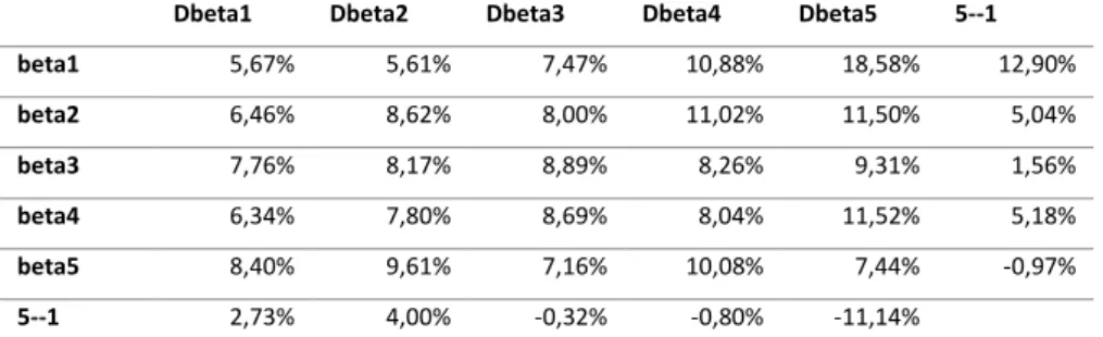
The results from the interception portfolios are quite intriguing. For portfolios with the same beta, if we increase the downside beta, we can note a pattern of increasing returns, consistent with previous literature. Specifically, for the portfolios with the lowest regular beta, sorting by downside betas, results in a major difference between top and bottom quintiles, at 12.90% (Table 4). One explanation may be because the stocks with low regular betas, will have a more stable beta throughout time, therefore, a sort by increasing downside beta will have a clearer impact on returns. This analysis only fails for the portfolio with high regular beta. Unlike the previous portfolios, the reason for this may be because in the high beta portfolios, the beta already accounts for the stocks with the highest downside betas, and therefore an additional sort by increasing downside beta, will not yield any improvement on the results. However, these stocks are naturally much more volatile and harder to predict. When analyzing the average returns for portfolios that increase in beta but hold downside beta constant, the highest downside beta portfolio stands out, as there is a decreasing pattern to be noticed, although not monotonic. The top and bottom quintiles yield 7.44% and 18.58% respectively, with a difference of -11.14% annually (Table 4). Here, it might be the case that for the highest downside beta
12
portfolios, the increase in beta is associated with an increase in upside betas, referring to stocks that are more correlated with positive market movements. Therefore, a higher upside beta would be in fact attractive for investors, who demand a lower premium for these stocks. It might be the case that this kind of breakpoint interception results in a very specific type of stock allocated in each portfolio. However, further analysis should be made to take better conclusions of these patterns.
Portfolios double sorted by unrestricted beta and downside beta:
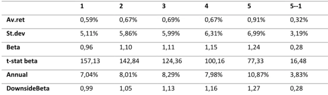
The results yield that the lowest downside beta portfolios, aggregated across regular betas, generate an annual return of 7.04%, while the highest downside beta portfolio generates about 10.87%. The difference between top and bottom quintile portfolios is at 3.83%, with a beta of 0.28 relevant with a t-stat of 16.48 (Table 7). Therefore, downside beta captures risk that is not priced by regular beta. Again, this should be expected because as I stated before, there should be a premium for holding stocks with higher downside risk, over stocks that are less correlated with the market in downturns. Note that the post-formation downside betas through portfolios 1 to 5, have a monotonically increasing pattern. What is important to note is that also their unconditional beta values show the same pattern, which the aggregation across regular betas would not have predicted. Therefore, by doing this, the betas and downside betas of these portfolios are intrinsically linked.
Portfolios sorted normal betas:
For these portfolios, sorted by the normal beta, we can see there is a monotonic increase pattern of the average returns. Annually, the top quintile portfolio generates 10.68% versus 7.72% generated by the bottom quintile portfolio. This puts the difference between top and bottom quintile at 2.96%, with a beta of 0.66 significant with a t-stat of 25.31 (Table 8). For the normal beta, we can also note that there is also a strictly monotonic increase of the post-formation beta,
13
letting us conclude that the normal beta portfolios, have predictive power of future betas and future returns. However, if we dissect the betas between the both extreme positive and extreme negative betas, we reach different conclusions as we did for the unrestricted portfolios when we separated the upside and downside betas. We can see from Graph 5 that these portfolios sorted on normal beta seem to be more sensitive to periods when the market return is below the lower band (beta of 0.0455), and less sensitive to periods when the market is above the higher band (beta of 0.0247), compared to periods when the market returns is between that range (beta of 0.0428). This further proves that negative periods are of more concern for investors. Just like previously for the downside beta, this extreme negative beta does explain cross sectional average excess returns slightly better than the normal beta, as the alpha when using extreme negative betas decreases to 0.0445, from 0.048 observed by using normal betas (Graph 5). However, the validity of the analysis for extreme negative and positive periods is called into question when we see that the number of observations for periods when the market return is below the extreme negative band, is cut to around one tenth of the total number of observations.
Portfolios sorted extreme positive betas and extreme negative betas:
For the extreme positive beta case, this analysis will change. Here it is possible to see that the difference between top and bottom quintile yields a negative average return of -0.92%, with a beta of 0.31 significant with a t-stat of 11.67 (Table 9). Again, this finding is evidence that upside volatility is good and attractive for investors, therefore reporting a negative risk premium for this factor. Reason being that a higher correlation with a growing market gives the investor a higher rate of return, while a higher correlation with a declining market is unattractive for investors because it will cause them to lose money when they need it the most.
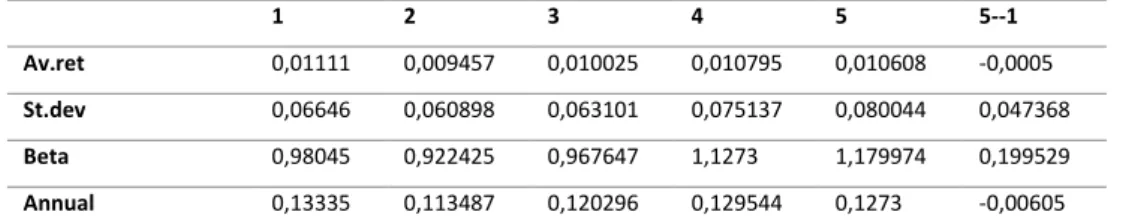
For the downside volatility market, there is no clear pattern that arises from this extreme negative beta sorts. Even though the difference between top and bottom quintile yields a
14
positive average return, it returns only 1.01% on average (Table 10). In fact, the fourth quintile is the portfolio that has the lowest average return, followed by the second quintile. Therefore, there is no consistency in returns using this sorting routine, and no advantage in forming portfolios sorted on extreme negative betas.
Portfolios sorted on normal betas (two standard deviations)
When considering two standard deviations to define extreme moments, the analysis does not change much from then I considered only one standard deviation. The average excess returns and betas both have an increasing pattern. The lowest quintile portfolio yields 7.90% per year, while the top quintile portfolio yields 11.27%. This puts the difference between top and bottom quintile at 3.37% (Table 11), which is an increase from the difference when sorting portfolios on normal beta, as reported above. Again, if we consider only the extreme negative betas of the portfolios, the alpha will decrease from 0.0529 from the new normal beta, to 0.0402, while the alpha increases to 0.0637 for the extreme upside betas. I also observe that average returns are more sensitive to periods when the market return is below the lower band, and less sensitive to periods when the market return is above the higher band (Graph 8).
Portfolios sorted on extreme positive and extreme negative betas (two standard deviations)
For these portfolios I will provide the results in Tables 12 and 13, but will not provide any conclusion on these sorts because the data for more extreme markets will be very limited. During the construction I was able to see that for a more volatile downstate market conditions, only half of the betas were able to be computed, thus affecting the quintile construction and monthly returns. This is even more evident for periods of more volatile upside market conditions. For these portfolios, there is only returns for 124 months, compared to around the 1019 months we analyze. This is because markets do not have very volatile periods for very long, whereas a normal market can be sustained for a very long time. Naturally, this problem
15
was not verified for the new normal betas, as expected, because as we use a two standard deviation band, by construction, more observations will fall into that range.
Conclusion
The purpose of this research was to analyze the impact of different betas, measured by the market past average return and its standard deviation over the same period. To do so we separated this paper in two parts. Part I focuses on previous literature, by breaking down beta into upside and downside beta first and replicating previous findings. The goal was to not only try to understand if downside beta accounts for average returns better than the CAPM, but also whether past-beta sorted portfolios forecast future downside betas and returns. As expected, I obtained results consistent with previous literature that investors place a higher importance on downside beta. I also find that after portfolio construction, if we were to apply a zero-cost investment strategy that goes long the high beta stocks and shorts the low beta stocks, there will be both statistically and economically significant returns generated. This difference is 4.74% for the top minus bottom deciles, sorted by unrestricted beta, decreases to 3.71% for the portfolios sorted on upside beta, and increases slightly to 5.01% for portfolios sorted on downside beta. And thus, concluding that downside beta is a more relevant measure of systematic risk. Part II focuses on the new analysis on normal beta, which I define by being within one standard deviation of returns, and extreme positive and extreme negative betas, defined by when the market return is outside these bands. For these portfolios sorted on normal betas, we note a similar pattern of increasing average returns and the difference between top and bottom quintiles is significant and returns 2.96% annually. I find that these portfolios, are also more sensitive to extreme negative periods, and less sensitive to extreme upside periods. This finding gives further strength that investors care more about the extreme downside periods
16
when compared to extreme upside periods. Again, investors give a bigger importance to extreme market downturns because it is when they need money the most. However, a sort on betas for extreme downside or extreme upside market periods do not produce any improvement in returns. Finally, I redefine the normal beta period using two standard deviation bands instead of one standard deviation. This essentially, increases the number of observations for the normal beta, but further decreases the number of observations for extreme cases. Thus, no conclusion can be made by using extreme market betas as the number of observations for these periods is very limited. For the portfolios sorted on the new normal beta measure however, the difference between top and bottom deciles increases from 2.96% to 3.37% annually.
In short, I find that none of the new measures provides an improvement over the downside risk model that generates a mean spread of 5.01%.
Issues and further research directions
For the purpose of this paper we did not account for several other characteristics that might have an effect on the stocks. For a deeper analysis and understanding, the researcher should take into account several other well-known characteristics such as size, book-to-market, momentum, volatility, coskewness, cokurtosis, liquidity, and others. Another problem across papers is regarding to betas. The beta estimates will differ from the true betas of different companies as this model does not take into account specific events, such as a firm levering up, increasing its risk and true beta. One last consideration is left to be made. Even though stock aggregation into portfolios provides a much easier analysis, Ang, Liu and Schwarz (2017) find that aggregation of stocks does not result into better estimates. Rather, by aggregating them, we are losing relevant information.
I want also to refer to the fact that despite all the support Downside CAPM has gotten, it is not a model consistent with diversification purposes and portfolio theory, as Cheremushkin (2009)
17
finds that semi-variance fails to account for the upside potential returns to hedge against downside returns of another stock.
For future research other methodologies may be applied in order to further analyze this asymmetric beta idea and correct for the missing observations on the extreme market conditions case. It could perhaps, instead of constructing deciles based on periods when the market return is below (above) the average market return minus (plus) one standard deviation, construct them using a symmetric percentile approach. For example, define these extreme conditions as the sensitivity to market returns being below the 20th percentile or above the 80th percentile of the market returns for the past three years.
18 References
Ang, A., Chen, J., & Xing, Y. (2001). “Downside risk and the momentum effect”. NBER Working Paper No. w8643.
Post, T., Van Vliet, P., & Lansdorp, S., (2009). “Sorting Out Downside Beta”. 22nd Australasian Finance and Banking Conference 2009.
Chen, J., Ang, A., & Xing, Y. (2005). “Downside Risk”. NBER Working Paper No. w11824. Cheremushkin, S. (2009). “Why D-CAPM is a Big Mistake? The Incorrectness of the Cosemivariance Statistics”
Dobrynskaya, V. (2010) “Downside Market Risk of Carry Trades”.
Fama, F., & French, R. (2003) “The Capital Asset Pricing Model: Theory and Evidence” CRSP Working Paper No. 550; Tuck Business School Working Paper No. 03-26.
Lettau, M., Maggiori, M., & Weber, M. (2014). “Conditional risk premia in currency markets and other asset classes”. Journal of Financial Economics, Elsevier, vol. 114(2), pages 197-225. Korn, O., & Kuntz, L., (2015) “Low-Beta Investment Strategies”.
Levi, Y., & Welch, I. (2017) “Market-Beta and Downside Risk”.
Ang, A., Chen, J., & Xing, Y. (2002). “Downside Correlation and Expected Stock Returns”. USC Finance & Business Econ. Working Paper No. 01-25.
Post, T., Van Vliet, P. (2004). “Conditional Downside Risk and the CAPM”. ERIM Report Series Reference No. ERS-2004-048-F&A.
Guy, A. (2014). “Upside and Downside Beta Portfolio Construction: A Different Approach to Risk Measurement and Portfolio Construction”.
Groenewald, N., & Fraser, P. (2003). “Forecasting Beta: How Well Does the ‘Five‐Year Rule of Thumb’ Do?”. Journal of Business Finance & Accounting. Volume 27, Issue 7-8, Pages 953-982.
19
Baker, M., Bradley, B., & Taliaferro, R. (2013). “The Low Risk Anomaly: A Decomposition into Micro and Macro Effects”. Financial Analysts Journal, Forthcoming.
Longin, F., & Solnik, B. (1999). “Correlation structure of international equity markets during extremely volatile periods”.
Patton, A., & Timmerann, A. (2008). “Portfolio Sorts and Tests of Cross-Sectional Patterns in Expected Returns”.
Dobrynskaya, V. (2014). “Asymmetric risk of momentum strategies”. Liu, J. (2016). “A novel measure of downside risk and expected returns”.
Galagedera, D., Brooks, R. (2005). “Is Systematic Downside Beta Risk Really Priced? Evidence in Emerging Market Data”.
Estrada, J. (2007). “Mean-Semivariance behaviour: Downside Risk and capital asset pricing”. International Review of Economics and Finance 16 (2007) 169-185.
Abbas, Q., Ayub, U., Sargana, S. & Saeed, S. (2011) “From Regular-Beta CAPM to Downside-Beta CAPM”. European Journal of Social Sciences, Vol. 21, No. 2, pp. 189-203, 2011. Le Bris, D. (2010). “What is a Market Crash?”. Paris December 2010 Finance Meeting EUROFIDAI - AFFI.
Atilgan, Y., Bali, T., Demirtas, K., Ozgur & Gunaydin, A. (2015. “Downside Beta and Equity Returns around the World”. Georgetown McDonough School of Business Research Paper No. 2798580.
Huffman, S., & Moll, C. (2012). “The Impact of Asymmetry on Expected Stock Returns: An Investigation of Alternative Risk Measures”. Algorithmic Finance (2012), 1:2, 79-93.
O’Malley, B. (2013) “A comparison of the forecasting accuracy of the Downside Beta and Beta on the JSE Top 40 for the period 2001-2011”.
Sharpe, W. (1964). “Capital Asset Prices: A Theory of Market Equilibrium under Conditions of Risk”. The Journal of Finance, Vol.19, No.3, pp. 425-442.
20
Fama, E., & French, K. (1993). “Common risk factors in the returns on stocks and bonds”. Journal of Financial Economics, Vol 33, Issue 3, Pages 3-56.
Roy, A. (1952). “Safety first and the holding of assets”. Econometrica, Vol.20, No. 3, pp. 431-449.
Markowitz, H. (1959), “Portfolio Selection: Efficient Diversification of Investments”. New Haven. Yale University Press.
Pedersen, C., & Hwang, S. (2007). “Does downside beta matter in asset pricing?”. Applied Financial Economics, 17:12, 961-978.
Kahneman, D., & A. Tversky. (1979). “Prospect Theory: An Analysis of Decision Under Risk,” Econometrica, 47, 263-291.
Gul, F. (1991). “A Theory of Disappointment Aversion,” Econometrica, 59, 3, 667-686. Jegadeesh, N., & Titman, S. (1993). “Returns to Buying Winners and Selling Losers: Implications for Stock Market Efficiency,” Journal of Finance, 48, 65-91.
Price, K., Price, B., & Nantell, T. J. (1982). “Variance and lower partial moment measures of systematic risk: some analytical and empirical results”. The Journal of Finance, 37(3), 843– 855.
Friend, I., & Blume, M. (1970). “Measurement of Portfolio Performance Under Uncertainty”. The American Economic Review, Vol. 60, No. 4, pp. 561-575.
Ang, A., Liu, J., & Schwarz, K. (2017). “Using Individual Stocks or Portfolios in Tests of Factor Models”. AFA 2009 San Francisco Meetings Paper.
Bhootra, A. (2011). “Are momentum profits driven by the cross-sectional dispersion in expected stock returns?”. Journal of Financial Markets, 14(3), 494-513.
Baker, M., Bradley, B., & Wurgler, J. (2010). “Benchmarks as Limits to Arbitrage: Understanding the Low Volatility Anomaly”. NYU Working Paper No. 2451/29593.
21 Appendix 1 2 3 4 5 6 7 8 9 10 10-1 Av.ret 0,46% 0,55% 0,63% 0,69% 0,76% 0,66% 0,74% 0,67% 0,72% 0,86% 0,39% St.dev 4,66% 4,39% 5,02% 5,49% 6,04% 6,34% 7,20% 7,56% 8,49% 10,18% 8,41% Beta 0,65 0,70 0,86 0,96 1,07 1,13 1,29 1,36 1,50 1,71 1,06 t-stat beta 34,54 48,90 63,59 72,19 77,32 81,28 83,17 86,92 74,36 58,39 28,08 Annual Ret 5,54% 6,57% 7,59% 8,27% 9,15% 7,94% 8,87% 8,04% 8,66% 10,28% 4,74% Upside beta 0,59 0,68 0,90 1,04 1,20 1,21 1,47 1,45 1,65 1,80 1,21 Downside beta 0,78 0,82 0,88 0,95 1,04 1,10 1,20 1,37 1,42 1,64 0,85
Table 1 – Statistics for portfolios sorted on unrestricted betas
1 2 3 4 5 6 7 8 9 10 10-1 Av.ret 0,52% 0,56% 0,63% 0,64% 0,64% 0,73% 0,78% 0,63% 0,72% 0,94% 0,42% St.dev 5,30% 4,68% 5,05% 5,29% 5,66% 5,96% 6,55% 7,11% 7,96% 9,44% 7,24% Beta 0,80 0,78 0,89 0,95 1,01 1,06 1,17 1,25 1,39 1,54 0,73 t-stat beta 41,79 57,30 75,46 83,43 82,61 77,49 82,68 74,59 70,94 52,06 20,18 Annual Ret 6,24% 6,75% 7,55% 7,68% 7,68% 8,71% 9,34% 7,61% 8,60% 11,25% 5,01% Downside beta 0,89 0,85 0,88 0,93 1,01 1,03 1,15 1,26 1,32 1,60 0,70
Table 2 – Statistics for portfolios sorted on downside beta
1 2 3 4 5 6 7 8 9 10 10-1 Av.ret 0,56% 0,61% 0,64% 0,67% 0,66% 0,72% 0,71% 0,68% 0,75% 0,87% 0,31% St.dev 5,76% 5,05% 5,13% 5,20% 5,70% 6,00% 6,45% 6,92% 7,45% 8,72% 6,47% Beta 0,88 0,82 0,87 0,92 1,01 1,07 1,15 1,24 1,32 1,45 0,57 t-stat beta 42,11 50,62 60,12 75,18 76,59 80,51 81,09 82,24 76,02 55,62 16,76 Annual Ret 6,73% 7,31% 7,70% 8,08% 7,88% 8,59% 8,47% 8,17% 8,95% 10,43% 3,70% Upside beta 0,81 0,80 0,87 0,94 1,11 1,10 1,22 1,41 1,41 1,48 0,67
Table 3 – Statistics for portfolios sorted on upside beta
Dbeta1 Dbeta2 Dbeta3 Dbeta4 Dbeta5 5--1 beta1 5,67% 5,61% 7,47% 10,88% 18,58% 12,90% beta2 6,46% 8,62% 8,00% 11,02% 11,50% 5,04% beta3 7,76% 8,17% 8,89% 8,26% 9,31% 1,56% beta4 6,34% 7,80% 8,69% 8,04% 11,52% 5,18% beta5 8,40% 9,61% 7,16% 10,08% 7,44% -0,97% 5--1 2,73% 4,00% -0,32% -0,80% -11,14%
Table 4 – Average returns for each interception of regular and downside beta portfolios
Dbeta1 Dbeta2 Dbeta3 Dbeta4 Dbeta5 beta1 0,67 0,71 0,77 0,86 1,14 beta2 0,98 0,88 0,89 1,01 0,86 beta3 1,13 1,05 1,07 1,18 1,28 beta4 1,23 1,33 1,32 1,29 1,38 beta5 1,15 1,45 1,49 1,47 1,68
22 Dbeta1 Dbeta2 Dbeta3 Dbeta4 Dbeta5
beta1 0,79 0,73 0,85 0,87 0,99 beta2 0,87 0,88 0,91 1,09 0,95 beta3 1,22 1,03 1,06 1,12 1,26 beta4 1,26 1,22 1,22 1,36 1,42 beta5 1,39 1,46 1,30 1,40 1,64
Table 6 – Post-formation downside betas for each interception of regular and downside beta portfolios
1 2 3 4 5 5--1 Av.ret 0,59% 0,67% 0,69% 0,67% 0,91% 0,32% St.dev 5,11% 5,86% 5,99% 6,31% 6,99% 3,19% Beta 0,96 1,10 1,11 1,15 1,24 0,28 t-stat beta 157,13 142,84 124,36 100,16 77,33 16,48 Annual 7,04% 8,01% 8,29% 7,98% 10,87% 3,83% DownsideBeta 0,99 1,05 1,13 1,16 1,27 0,28
Table 7 – Statistics for portfolios double sorted on regular and downside beta and aggregated across regular betas
1 2 3 4 5 5--1 Av.ret 0,64% 0,71% 0,83% 0,86% 0,89% 0,25% St.dev 4,54% 4,58% 5,48% 6,66% 7,70% 5,23% Beta 0,79 0,86 1,06 1,28 1,45 0,66 t-stat beta 54,14 83,34 101,51 95,33 80,57 25,31 Annual 7,72% 8,57% 9,95% 10,31% 10,68% 2,96% +extreme beta 0,65 0,81 1,14 1,65 1,71 1,06 -extreme beta 0,85 0,91 1,03 1,26 1,44 0,60
Table 8 – Statistics for portfolios sorted on normal moments betas
1 2 3 4 5 5--1 Av.ret 0,88% 0,76% 0,76% 0,74% 0,80% -0,08% St.dev 5,28% 4,66% 4,99% 5,51% 6,75% 4,45% Sharpe 0,17 0,16 0,15 0,14 0,12 -0,02 Beta 0,89 0,84 0,92 1,02 1,20 0,31 Annual 10,53% 9,12% 9,15% 8,92% 9,61% -0,92% +extreme betas 0,75 0,77 1,09 1,25 1,40 0,65
Table 9 – Statistics for portfolios sorted on extreme positive market betas
1 2 3 4 5 5--1 Av.ret 0,71% 0,69% 0,78% 0,62% 0,80% 0,08% St.dev 5,03% 4,61% 5,14% 5,69% 7,18% 4,82% Sharpe 0,14 0,15 0,15 0,11 0,11 0,02 Beta 0,89 0,87 0,98 1,08 1,30 0,42 Annual 8,54% 8,23% 9,37% 7,39% 9,55% 1,01% -extremebetas 0,93 0,95 0,97 1,19 1,30 0,37
23 y = 0,0328x + 0,044 0,00% 2,00% 4,00% 6,00% 8,00% 10,00% 12,00% 0,50 1,00 1,50 2,00 Unrestricted betas y = 0,029x + 0,0462 0,00% 2,00% 4,00% 6,00% 8,00% 10,00% 12,00% 0,50 1,00 1,50 2,00 Upside betas y = 0,0369x + 0,0396 0,00% 2,00% 4,00% 6,00% 8,00% 10,00% 12,00% 0,50 0,70 0,90 1,10 1,30 1,50 1,70 Downside betas 1 2 3 4 5 5--1 Av.ret 0,66% 0,72% 0,82% 0,81% 0,94% 0,28% St.dev 4,08% 4,86% 5,84% 6,76% 8,37% 6,18% Beta 0,68 0,92 1,12 1,30 1,56 0,87 t-stat beta 47,58 87,58 97,76 98,79 76,32 31,28 Annual 7,90% 8,61% 9,80% 9,76% 11,27% 3,37% +2extremebeta 0,59 0,94 1,34 1,51 1,94 1,35 -2extremebeta 0,87 0,97 1,08 1,27 1,52 0,65
Table 11 – Statistics for portfolios sorted on normal betas (two standard deviations)
1 2 3 4 5
Av.ret 0,01056 0,01124 0,009635 0,011815 0,009073 -0,003 St.dev 0,07737 0,061087 0,055248 0,079091 0,07587 0,012751 Beta 1,16658 0,938008 0,84272 1,214269 1,135253 -0,02928 Annual 0,12676 0,134878 0,115624 0,14178 0,108879 -0,03596
Table 12 – Statistics for portfolios sorted on extreme positive market betas
1 2 3 4 5 5--1
Av.ret 0,01111 0,009457 0,010025 0,010795 0,010608 -0,0005 St.dev 0,06646 0,060898 0,063101 0,075137 0,080044 0,047368 Beta 0,98045 0,922425 0,967647 1,1273 1,179974 0,199529 Annual 0,13335 0,113487 0,120296 0,129544 0,1273 -0,00605
Table 13 – Statistics for portfolios sorted on extreme positive market betas
24 y = 0,0479x + 0,0294 0,00% 2,00% 4,00% 6,00% 8,00% 10,00% 12,00% 0,50 0,70 0,90 1,10 1,30 1,50 1,70 Unrestricted betas y = 0,0495x + 0,0272 0,00% 2,00% 4,00% 6,00% 8,00% 10,00% 12,00% 0,50 0,70 0,90 1,10 1,30 1,50 1,70 Downside betas y = 0,0415x + 0,0378 0,00% 2,00% 4,00% 6,00% 8,00% 10,00% 12,00% 0,50 0,70 0,90 1,10 1,30 1,50 Unrestricted betas y = 0,0324x + 0,0462 0,00% 2,00% 4,00% 6,00% 8,00% 10,00% 12,00% 0,50 0,70 0,90 1,10 1,30 1,50 1,70 Upside betas y = 0,1249x - 0,0547 0,00% 2,00% 4,00% 6,00% 8,00% 10,00% 12,00% 0,90 1,00 1,10 1,20 1,30 Unrestricted betas y = 0,1216x - 0,0517 0,00% 2,00% 4,00% 6,00% 8,00% 10,00% 12,00% 0,90 1,00 1,10 1,20 1,30 Downside betas y = 0,0428x + 0,048 0,00% 2,00% 4,00% 6,00% 8,00% 10,00% 12,00% 0,50 0,70 0,90 1,10 1,30 1,50 Unrestricted betas y = 0,0247x + 0,065 0,00% 2,00% 4,00% 6,00% 8,00% 10,00% 12,00% 0,50 0,70 0,90 1,10 1,30 1,50 1,70 1,90
Extreme positive market betas
y = 0,0455x + 0,0445 0,00% 2,00% 4,00% 6,00% 8,00% 10,00% 12,00% 0,50 0,70 0,90 1,10 1,30 1,50 Extreme negative market betas
Graph 2 – Plot of average returns vs. Beta and downside beta for portfolios sorted on downside betas.
Graph 3 – Plot of average returns vs. Beta and upside beta for portfolios sorted on upside betas.
Graph 4 – Plot of average returns vs. Beta and downside beta for portfolios double on beta and downside beta.
Graph 5 – Plot of average returns vs. beta, extreme positive market beta and extreme negative market beta for portfolios sorted on normal betas.
25 y = -0,0018x + 0,0964 8,50% 9,00% 9,50% 10,00% 10,50% 11,00% 0,50 0,70 0,90 1,10 1,30 Unrestricted betas y = -0,009x + 0,1041 8,50% 9,00% 9,50% 10,00% 10,50% 11,00% 0,50 0,70 0,90 1,10 1,30 1,50
Extreme positive market betas
y = 0,0184x + 0,0673 0,00% 2,00% 4,00% 6,00% 8,00% 10,00% 12,00% 0,70 0,80 0,90 1,00 1,10 1,20 1,30 1,40 Unrestricted betas y = 0,0051x + 0,0807 0,00% 2,00% 4,00% 6,00% 8,00% 10,00% 12,00% 0,70 0,80 0,90 1,00 1,10 1,20 1,30 1,40
Extreme negative market betas
y = 0,0374x + 0,0529 0,00% 2,00% 4,00% 6,00% 8,00% 10,00% 12,00% 0,50 0,70 0,90 1,10 1,30 1,50 1,70 Unrestricted betas y = 0,0245x + 0,0637 0,00% 2,00% 4,00% 6,00% 8,00% 10,00% 12,00% 0,50 1,00 1,50 2,00 2,50
Extreme positive market betas
y = 0,0477x + 0,0402 0,00% 2,00% 4,00% 6,00% 8,00% 10,00% 12,00% 0,50 0,70 0,90 1,10 1,30 1,50 1,70
Extreme negative market betas
Graph 6 – Plot of average returns vs. Beta and extreme positive market beta for portfolios sorted on extreme positive market betas.
Graph 7 – Plot of average returns vs. Beta and extreme negative market beta for portfolios sorted on extreme negative market betas.
Graph 8 – Plot of average returns vs. beta, extreme positive market beta and extreme negative market beta for portfolios sorted on normal betas (two standard deviations).