Comparison of Different Interpolation Techniques to Map
Temperature in the Southern Region of Eritrea
Mussie G. Tewolde, Teshome A. Beza, Ana Cristina Costa, Marco Painho
Instituto Superior de Estatística e Gestão de Informação, Universidade Nova de Lisboa { [email protected]; [email protected]; [email protected];
INTRODUCTION
Temperature and rainfall vary markedly throughout Eritrea, from hot desert in the east to a mild, subhumid climate in the highlands (Wolfe et al., 2008). Prediction and understanding of the spatial variation of climate data, particularly temperature, is important to many agricultural and economic sectors for planning and management activities (Moral, 2009). This is especially important in Eritrea where agriculture provides 12.4% of the gross domestic product, and 80% of the population are involved in farming and herding (Wolfe et al., 2008).
Several studies have demonstrated that various spatial interpolation techniques perform differently depending on the type of attribute, geometrical configuration of the samples, spatial resolution, world region, etc. (Martínez-Cob, 1996; Goovaerts, 2000; Haberlandt, 2007). Hence, selecting the best interpolation technique for each particular situation is a key factor. The major objective of this study is to assess the spatial variability of annual average temperature in the southern region of Eritrea by comparing different interpolation procedures. The temperature data were interpolated using a deterministic method (Inverse square distance) and three geostatistical methods (Ordinary, Universal and Simple kriging). The performance of the different techniques was compared through error statistics computed using Jackknife cross-validation.
METHODS
Inverse Distance Weighting (IDW) is a (quick) exact deterministic interpolator that requires very few decisions regarding model parameters, because it accounts for distance relationships only. This method assigns weights in an averaging function based on the inverse of the distance (raised to some power) to every data points located within a given search radius centred on the point of estimate. In this study, the most common formula was used by considering a power of two, thus the method is sometimes named Inverse Square Distance.
Kriging is a group of geostatistical techniques used to estimate the value of a random field at an unobserved location using a set of samples from nearby locations. The kriging estimators are variants of the basic linear regression estimator:
[
]
∑
= α α α α−
λ
=
−
) x ( N 1 0 0 0 0)
x
(
m
)
x
(
z
)
x
(
)
x
(
m
)
x
(
*
Z
(1)where λα(x0) is the weight assigned to datum z(xα); m(x0) and m(xα) are the expected values of the random variables Z(x0) and Z(xα); N(x0) is the number of samples closest to the location x0 being estimated.
When developing the kriging equations, the variogram model (inverse function of the spatial covariances) is assumed known. Typically, a mathematical semivariogram model is selected from a small set of authorized ones and is fitted to experimental semivariogram values calculated from data for given angular and distance classes. The most common models are the spherical, exponential and Gaussian models (Goovaerts, 1997; Prudhomme and Reed, 1999). Here, we considered an isotropic exponential model, with the range parameter equal to 16Km and the sill parameter equal to 28.081.
The kriging estimator varies depending on the model adopted for the random function Z(xα) itself, which is usually expressed as
Z(xα) = R(xα) + m(xα), ∀xα (2) where R(xα) is the residual component, and m(xα) is the trend component.
Three kriging variants can be distinguished according to the model considered for the trend m(xα): Simple kriging (SK), Ordinary kriging (OK), and Universal kriging (UK), which is also known as Kriging with a trend model. The m(xα) is assumed known and constant throughout the study area in SK, while OK accounts for local variations of the mean by limiting its domain of stationarity to a local neighbourhood. In UK, the trend component is modelled as a linear combination of functions of the spatial coordinates.
STUDY REGION AND DATA
The study region is located in the southern part of Eritrea (Fig 1). The country is located in the northeastern part of Africa between the latitudes 124°42’ North and 18°2’ North, and the longitudes 36°30’ East and 43°20’ East. The data were obtained from the Ministry of Land, Water and Environment, Water Resource Department (WRD). Average temperature records of 2005 were collected from monitoring stations located in 427 villages of the Southern region of Eritrea (Fig 1). Generally, the area is characterized by mild temperature conditions ranging from 10 to approximately 30 degrees Celsius. However, there are a few areas located in the east with high temperature records. Table 1 lists a few summary statistics of the collected data.
Figure 1: Location of the study region in Eritrea (right) and stations’ locations (left).
Table 1: Summary statistics of the temperature records
Sample statistics Value
Minimum 9.8°C Maximum 34.9°C Mean 23.03°C Median 23.30°C Standard deviation 5.31°C Variance 28.15 Kurtosis −0.67 Skewness −0.02
RESULTS AND DISCUSSION
The temperature maps (Fig. 2) were produced using the Geostatistical Analyst extension of ArcGIS© 9.3, while the variography analyses required for kriging was performed using the geoMS© – Geostatistical Modelling Software.
Figure 2: Annual temperature maps obtained using different interpolators: Inverse distance weighting
(IDW), Simple kriging (SK), Ordinary kriging (OK), Universal kriging (UK).
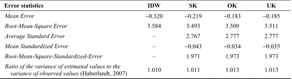
The error statistics of the different interpolation methods reveal that all techniques have a similar performance (Table 2). IDW is slightly less accurate and more biased than the kriging methods (as expected). However, in future studies, a demanding variogram analysis can be avoided by choosing the IDW approach. Hence, temperature data of other years can be easily and quickly interpolated using the IDW technique.
Table 2: Error statistics based on cross-validation for different interpolators
Error statistics IDW SK OK UK
Mean Error −0.320 −0.219 −0.183 −0.185
Root-Mean-Square Error 3.584 3.493 3.509 3.511
Average Standard Error – 2.767 2.777 2.777
Mean Standardized Error – −0.043 −0.034 −0.035
Root-Mean-Square-Standardized-Error – 1.971 1.973 1.973
Ratio of the variance of estimated values to the
variance of observed values (Haberlandt, 2007) 1.010 1.011 1.013 1.013
Using elevation data in the estimation process is likely to be beneficial, especially in mountainous areas (Vicente-Serrano et al., 2003). Accordingly, other techniques that make use of secondary information, such as Cokriging, should be evaluated in future studies if the stations’ altitude data is available.
REFERENCES
Goovaerts P., Geostatistics for Natural Resources Evaluation, Applied Geostatistics Series, Oxford University Press, 1997.
Goovaerts P., Geostatistical approaches for incorporating elevation into the spatial interpolation of rainfall, J. Hydrol. 228: 113-129, 2000.
Haberlandt U., Geostatistical interpolation of hourly precipitation from rain gauges and radar for a large-scale extreme rainfall event, J. Hydrol. 332: 144-157, 2007.
Martínez-Cob A., Multivariate geostatistical analysis of evapotranspiration and precipitation in mountainous terrain, J. Hydrol. 174: 19-35, 1996.
Moral, F. J., Comparison of different geostatistical approaches to map climate variables: application to precipitation, Int. J. Climatol. DOI: 10.1002/joc.1913, 2009.
Prudhomme C., Reed D. W., Mapping extreme rainfall in a mountainous region using geostatistical techniques: a case study in Scotland, Int. J. Climatol. 19(12): 1337-1356, 1999.
Vicente-Serrano S. M., Saz-Sánchez M. A., Cuadrat J. M., Comparative analysis of interpolation methods in the middle Ebro Valley (Spain): application to annual precipitation and temperature, Climate Research 24(2): 161-180, 2003.
Wolfe E. C., Tesfai T., Cook B., Tesfay E., Bowman A., “Forages for agricultural production and catchment protection in Eritrea”. In: M. Unkovich (Ed.), Global Issues, Paddock Action:
Proceedings of the 14th Australian Agronomy Conference, Adelaide, South Australia,