Development of an analysis pipeline for human microelectrode recordings in Parkinson’s disease

(1)

Instituto Politécnico de Lisboa

Instituto Superior de Engenharia de Lisboa

Escola Superior de Tecnologia da Saúde de Lisboa

Development of an analysis pipeline for human

microelectrode recordings in Parkinson’s Disease

Sara Fernández Abalde

Thesis to obtain the Master Degree in Biomedical Engineering

Supervisors: Gonçalo Caetano Marques (ISEL) Marcelo Mendonça (Fundação Champalimaud)

Examination Committee

Chairperson: João Costa, PhD

Members of the Committee: André Caetano, MD João Sousa, PhD

Marcelo Mendonça, MD

(2)

(3)

Development of an analysis pipeline for human microelectrode

recordings in Parkinson’s Disease

Sara Fernández Abalde

This work was performed at Neurobiology of Action Lab in Champalimaud Center for the Unknown, led by Rui Costa, DVM, PhD under the direct supervision of Marcelo Mendonça, MD in the scope of the Master Thesis in Biomedical Engineering of ISEL-Instituto Superior de Engenharia de Lisboa and ESTeSL- Escola Superior de Tecnologia da Saúde de Lisboa.

(4)

(5)

Acknowledgments

I want to thank my supervisors Marcelo and Gonçalo for their advice, knowledge, patience, help and different perspectives during this whole work.

Thank you to Cecilia Calado for all the given opportunities, availability and information since the first year of the master degree.

I would like to thank Rui Costa for the opportunity of joining the Neurobiology of Action Lab in Champalimaud Center for the Unknown. Special acknowledgments to all people who is part of the Costa lab and this inspiring workplace. Your science is awesome and you motivated me, inspired me and triggered my interest in neuroscience research. Also I want to thank especially Ricardo Matias for his help. Moreover, I would like to thank Albino Oliveira-Maia and the Neuropsychiatry Unit of the Champalimaud Foundation for your attention, help and for inviting me to learn with you all during your meetings.

I want to acknowledge all people in CHLO Movements Disorders Surgery Group (Raquel Barbosa, Alexandra Seromenho-Santos, Pedro Pires, Carla Reizinho and Paulo Bugalho) for their amazing work helping people, which made possible this project.

Finally, thanks to my family and Torgny, since all of this couldn’t have been possible without your support.

(6)

(7)

Abstract

Background:

Deep brain stimulation is a common treatment for advanced Parkinson’s Disease (PD). Intra-operative microelectrode recordings (MER) along preplanned trajectories are often used for ac-curate identification of subthalamic nucleus (STN), a common target for deep brain stimula-tion (DBS) in PD. However, this identificastimula-tion is performed manually and can be difficult in regions of transition. Misidentification may lead to suboptimal location of the DBS lead and inadequate clinical outcomes.

Methods:

A tool for unsupervised analysis and spike-sorting of human MER signals with feature extrac-tion was developed. We also trained and tested a hybrid unsupervised/supervised machine learn-ing approach that uses extracted MER time, frequency and noise properties for high-accuracy identification of STN. Lastly, we compared neurophysiological characteristics of different STN functional segments.

Results:

We obtained a classification accuracy of 96.28 ± 3.15 % (30 trajectories, 5 patients) for individual STN-DBS surgery MER using an approach of "leave one subject out" validation with support vector machine classifier, all features based on time and frequency domain and human expert labels.

The unsupervised sorting approach allowed us to sort a total of 357 STN neurons in 5 sub-jects. Dividing the STN in a dorsal, probably motor region, and a ventral, probably non-motor portion, we’ve found a higher burst rate (median (interquartile range) of 1.8 (1.5) vs 1.15 (0.05) bursts/s, p=0.001) and firing rate (median (interquartile range) of 21.4 (16.85) vs. 15.3 (14.33), p=0.013) of dorsal STN neurons among other features. Ongoing work will refine these results using anatomical gold standard through lead trajectory reconstruction, fused with an STN func-tional subdivision atlas.

Conclusions:

(8)

provided good preliminary results in STN classification. In line with the literature, we were able to find preliminary activity differences in functionally segregated STN segments. This tool is fast and generalizable for other brain regions. Ongoing work using patient’s anatomy can further validate its’ usefulness in optimizing electrode placement and research purposes.

Keywords

Microelectrode Recordings (MER); Deep Brain Stimulation (DBS); Parkinson’s Disease (PD); Subthalamic Nucleus (STN); Support Vector Machines (SVM)

(9)

Resumo

A Estimulação Cerebral Profunda é um técnica utilizada para o tratamento dos sintomas motores da Doença de Parkinson com recurso a estimulação eléctrica intracraniana. Um dos alvos mais frequentemente utilizados para o tratamento é o núcleo subtalâmico e uma colocação precisa dos eléctrodos na região correcta é fulcral para o sucesso terapêutico e minimização de efeitos secundários.

Esta cirurgia faz-se com recurso a estereotaxia e monitorização intra-operatória. Previamente à cirurgia, as coordenadas do alvo são estabelecidas e é definido o núcleo subtalâmico utilizando imagens pré-operatórias de ressonância magnética e de tomografia computadorizada do doente. Intra-operatoriamente são utilizados registos de microeléctrodos a diferentes profundidades em trajetórias pré-definidas para verificar as coordenadas estabelecidas e identificar -pela actividade eléctrica- a localização dos eléctrodos no cérebro. No entanto, a identificação do núcleo subta-lâmico com registos de microeléctrodos é frequentemente realizada por inspeção visual, e pode ser difícil em regiões de transição. Erros na identificação podem levar a um posicionamento subóptimo dos elétrodos e a um mau resultado clínico.

O correcto posicionamento do eléctrodo final de estimulação na porção sensoriomotora do núcleo subtalâmico está relacionado com os melhores resultados clínicos de acordo com a lite-ratura. No entanto não é possível identificar claramente esta subdivisão com base a inspecção visual dos registos.

O objetivo do presente estudo é o desenvolvimento de ferramentas para análise de registos de microeléctrodos em diferentes áreas do cérebro e identificação do núcleo subtalâmico, e da porção sensoriomotora, em doentes com Doença de Parkinson submetidos a estimulação cerebral profunda.

Métodos

Foram desenvolvidas ferramentas para análise do sinal, spike sorting e extração de caracte-rísticas por processamento não supervisionado de registos de microeléctrodos humanos.

As características relativas ao domínio do tempo e frequência foram obtidas para cada sinal através de medidas estatísticas (média, mediana e desvio padrão) dos registos fracionados em segmentos sobrepostos, para minimizar os efeitos do ruído. As características relacionadas com a

(10)

atividade neuronal foram também extraídas após deteção e identificação dos diferentes neurónios em cada registo de forma não supervisionada.

A localização dos diferentes registos ao longo do trajecto foi realizada por um especialista através de inspeção visual aleatória de todos os sinais. As características extraídas nas regiões do núcleo subtalâmico foram comparadas com as registadas fora de esta área.

Posteriormente, uma abordagem híbrida de classificação utilizando métodos de aprendizagem automática -machine learning- foi treinada e testada para identificação dos registos localizados no núcleo subtalâmico utilizando as características extraídas baseadas no domínio do tempo e frequência.

Para comparar as sub-regiões funcionais do núcleo subtalâmico, utilizaram-se os sinais identi-ficados em esta região e dividiram-se estas profundidades etiquetadas pelo especialista como nú-cleo subtalâmico na porção mais dorsal (que terá maior probabilidade de ser motora) e outra ven-tral (que terá maior probabilidade de ser não motora). Utilizando esta subdivisão, compararam-se as características neurofisiológicas relativas às diferentes sub-regiões funcionais com testes estatísticos.

Conhecendo as limitações da classificação por inspecção visual, desenvolveu-se uma meto-dologia para refinamento das localizações dos diferentes registos baseada na reconstrução da trajetória dos eléctrodos implantados, utilizando imagens pre- e pos- operatórias. Esta recons-trução foi sobreposta a um atlas contendo as subdivisões funcionais do núcleo subtalâmico. Os resultados preliminares desta aplicação num sujeito, permitiram mostrar uma classificação mais realista destas sub-regiões na identificação da área motora vs. não motora (límbica e associativa).

Resultados

Foram identificadas várias características significativamente diferentes no domínio do tempo e frequência, entre os sinais classificados como pertencentes ao Núcleo Subtalámico e os sinais não-pertencentes. Estas diferenças permitiram o desenvolvimento de classificadores do tipo de máquinas de vectores de suporte, utilizando as localizações dos diferentes registos tendo como base a classificação baseada em inspecção visual por um especialista.

Utilizando os sinais de maior certeza de classificação, obteve-se uma precisão de classificação do núcleo subtalâmico de 96,18 ± 3,15 % (para 30 trajetórias, 5 pacientes) usando uma abor-dagem de validação cruzada de “deixar um sujeito fora"com máquina de vectores de suporte linear. Este modelo de validação garante que os dados relativos aos doentes utilizados para trei-nar o modelo não foram usados posteriormente para testar o mesmo. Utilizando todos os sinais considerados como núcleo subtalâmico independentemente do nível de certeza, obteve-se uma classificação de 84,32 ± 5,75 %.

A ferramenta não supervisionada para spike sorting permitiu a identificação de um total de 357 neurónios do núcleo subtalâmico identificado com a máxima certeza em 5 doentes (155 registos de microeléctrodos de 10 segundos de duração) e 521 neurónios foram extraídos de 420

(11)

sinais localizados fora do núcleo subtalâmico. Utilizando segmentos de 10 segundos livres de artefactos, identificamos 258 neurónios em 116 sinais do núcleo subtalâmico e 329 neurónios em 228 registos de não-Subtalámico. Foram encontradas diferenças significativas em em 13 das 15 características analisadas comparando STN com não-STN.

As subregiões funcionais do núcleo subtalâmico (dorsal vs. ventral) foram comparadas quanto às caracteristicas de tempo, frequência e actividade neuronal. Encontraram-se diferenças signi-ficativas em 6 características extraídas dos sinais sem artefactos, consistentes com a literatura e também em uma característica de frequência. Em linha com o descrito previamente, encontra-mos um burts rate mais elevado na subdivisão dorsal em relação à ventral (mediana (amplitude interquartil) of 1.8(1.5) vs 1.15(0.05) bursts/s, p=0.001) e um firing rate mais alto (mediana (amplitude interquartil) of 21.4(16.85) vs. 15.3(14.33), p=0.013) entre outras características.

Os resultados preliminares da análise de sinal refinado por imagem num sujeito, mostraram uma alta accuracy do expert na classificação de sinais STN/não-STN comparados com imagem (>85%). Apesar de neste sujeito não se obterem diferenças significativas entre regiões nas ca-racterísticas extraídas, esta analise mostrou que divisão heurística dorsal/ventral era insuficiente para proceder à analise apropriada.

Conclusões

Foi desenvolvida uma ferramenta para análise de registo de microeléctrodos em humanos e para extração de características no domínio do tempo e frequência, que forneceu bons resultados na classificação do núcleo subtalâmico utilizando a identificação da localização de cada registo por um especialista.

A análise e extração de características relativas à atividade neuronal foi realizada por uma ferramenta não supervisionada, que foi desenvolvida combinando algoritmos existentes e que pode ser generalizável a registos em outras regiões ou outro tipo de registos. Esta ferramenta permitiu a identificação de características que permitem diferenciar os sinais colhidos no núcleo subtalâmico dos identificados fora de esta região.

De acordo com a literatura, fomos capazes de identificar diferenças em segmentos funcional-mente segregados do núcleo subtalâmico. O trabalho em curso, com refinação anatómica, vai-nos permitir avaliar a sua utilidade em optimizar o posicionamento dos elétrodos, podendo também ser utilizado para fins de investigação.

Palavras chave

Estimulação cerebral profunda; Doença de Parkinson; núcleo subtalâmico; registos de microeléc-trodos intraoperatórios; máquinas de vector de suporte

(12)

(13)

List of Figures

1.1 Circuity between basal ganglia motor structures in "normal" condition and PD . 3

1.2 Basal ganglia-thalamo-cortical circuitry in STN-DBS. . . 4

1.3 Subthalamic Nucleus and functional subdivisions . . . 5

1.4 Stereotactic frame and fiducial points. . . 6

1.5 Localization of intraoperative microelectrode recordings channels and segments of acquisitions at different depths. . . 7

1.6 DBS basic implanted components. . . 7

3.1 Segments of microelectrode recording (MER) shown for expert labelling. . . 12

3.2 Subdivision of STN-expert identified MER. . . 13

3.3 Normalization of CT to the MNI space. . . 14

3.4 Subcortical refinement on normalized images and location of masks. . . 15

3.5 Lead reconstruction interface based on patient’s images. . . 15

3.6 Axial view of STN subdivisions with reconstructed electrodes. . . 15

3.7 Filtered signal with elliptical band pass filter overlapped to raw MER. . . 16

3.8 Detection of artifacts in filtered signal. . . 17

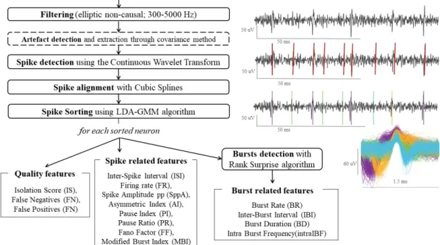
3.9 Workflow for MER analysis and extraction of time and frequency related features. 18 3.10 Workflow process of spike related features. . . 19

3.11 Spike train of detected spike events on the clean filtered signal. . . 20

3.12 Detected spikes in filtered MER after spike detection and sorting and their respec-tive overlapped waveforms. . . 21

3.13 Cross-validation iterations for leave one subject out approach . . . 24

4.1 Quality measures for the spike sorting results in segments free of artifacts. . . 32

4.2 Reconstruction of electrode’s trajectory based on patient’s imagiology. . . 37

5.1 Comparison of spike sorting performances . . . 42

D.1 Random Permutation tests between STN subdivisions for spike related features using 10 second filtered segments. . . 65

(16)

D.2 Random Permutation tests between STN subdivisions for spike related features using 10 second filtered segments free of artifacts. . . 66

(17)

List of Tables

3.1 Confusion matrix and related performance measures. . . 25

4.1 Characteristics of subjects, recording duration and MER depths. . . 27

4.2 Results of expert based classification of MER by visual inspection. . . 28

4.3 Time related features statistic results for MER filtered segments. . . 29

4.4 Statistics results of frequency related features for MER filtered segments. . . 30

4.5 Spike related statistical results for segments free of artifacts . . . 31

4.6 Classification results with 10-cross validation for STN maximum certainty. . . 33

4.7 Classification results with 10-cross validation for all STN labels. . . 33

4.8 Classification results for STN maximum certainty using 2 principal components (PCs) and 10-cross validation. . . 34

4.9 Classification results for STN maximum certainty using 4 PCs and 10-cross vali-dation. . . 35

4.10 Estimated accuracy percentage for leave-one-subject-out validation using STN maximum certainty. . . 35

4.11 Estimated accuracy percentage for leave-one-subject-out validation using all STN-MER. . . 36

4.12 Spike related features for artifact-free segments in STN subdivisions. . . 37

4.13 Results of labelling based on imagiology and expert visual inspection for one patient. 38 4.14 Confusion matrix for STN identification based on expert labels with certainty higher than 50% vs. anatomical gold standard. . . 39

4.15 Confusion matrix for STN identification based on all expert labels vs. anatomical gold standard. . . 39

B.1 Time and frequency related eatures for MER filtered segments free-of artifacts. . 58

B.2 Statistical results of spike related features in filtered MER to compare STN and non STN regions. . . 59

B.3 Statistical results of spike related features of fitered artifact-free MER with isola-tion score higher than 0.5. . . 60

(18)

C.1 Classification results using 2 PCs and 10-cross validation for all STN labels. . . . 61 C.2 Classification results using 4 PCs and 10-cross validation for all STN labels. . . . 62 D.1 Results of time and frequency related features for STN subdivisions based on

expert labels. . . 63 D.2 Statistic results of spike related features for STN subdivisions in filtered free of

artifact segments. . . 64 D.3 Statistical results of time and frequency features for STN subdivisions refined with

lead reconstruction. . . 67 D.4 Statistical results of spike related features for STN subdivisions refined with lead

(19)

Acronyms

AC anterior commisure AI assimetry index

ANTs Advanced Normalization Tools AP action potential BA basal ganglia BI burst index BR burst rate CF crest factor CT computed tomography CV cross validation

cvISI coefficient of variation of interspike interval CWT continuous wavelet transform

DARTEL Diffeomorphic Anatomical Registration Through Exponentiated Lie algebra DA dopamine

DBS deep brain stimulation

DICOM Digital Imaging and Communications in Medicine dSTN dorsal subthalamic nucleus

FF fano factor FN false negative

(20)

FP false positive FR firing rate

GMM gaussian mixture model GPe external Globus Pallidus GPi internal Globus Pallidus ISI interspike interval

IS isolation score

LDA linear discriminant analysis MAVS mean absolute value slope MAV mean absolute value

MBI modified burst index

MC Mel-frequency cepstral coefficients mdnBD median burst duration

mdnFRQ median frequency

mdnIBF median intraburst frequency mdnIBI median interburst interval mdnISI median interspike interval MER microelectrode recording mFRQ mean frequency

MNI Montreal Neurological Institute MRI magnetic resonance imaging PCA principal components analysis PC posterior commisure

PCs principal components PD Parkinson’s Disease

(21)

PI pause index PR pause ratio

PaCER Precise and Convenient Electrode Reconstruction for Deep Brain Stimulation RMS root mean square

RSA Rank Surprise algorithm SDN standard deviation of noise SF spectral flux

SNc Substantia Nigra pars compacta SPC spectral centroid

SPM12 Statistical Parametric Mapping 12 stdISI standard deviation of interspike interval STN subthalamic nucleus

SVM support vector machine SppA spike peak-to-peak amplitude TE Teager energy

TN true negatives TP true positives VAR variance

vSTN ventral subthalamic nucleus WL waveform of curve length ZC zero crossings

(22)

(23)

Chapter 1

Introduction

Deep Brain Stimulation (DBS) is a common treatment for advanced Parkinson’s Disease (PD). In this therapeutic technique, a small pair of electrodes is implanted surgically in a target area (subthalamic nucleus (STN) or the pars interna of Globus Pallidus (GPi)) to reverse motor symptoms through its stimulation.

During surgery, clinicians decide the final electrodes position based on different and com-plementary approaches: 1) target coordinates are defined prior to surgery based on patient’s pre-operative magnetic resonance imaging (MRI) and computed tomography (CT) imaging. 2) During surgery, intra-operative microelectrode recordings (MER) along the trajectory to the target are visually inspected, and borders of STN identified. 3) Afterwards, final lead position is reviewed through therapeutic and side effects assessment by intra-operative stimulation.

In STN-DBS, a proper placement of the final electrode and particularly stimulation within sensorimotor STN is related with the best clinical results. However, identification of this region on regular MRI is impossible and MER-based features that can distinguish clearly this region remain to be clarified.

In this study, we contribute to the development of clinical-decision support tools for target identification in STN-DBS, through computational analysis using intraoperative MER. Objec-tives are explained in depth in chapter 2, but theoretical background regarding Parkinson’s Dis-ease and STN-DBS is presented in the following section in order to provide better understanding of the problem and purpose of our study.

1.1 Parkinson’s Disease

Parkinson’s Disease is the second most common neurodegenerative disease worldwide. It is a chronic and progressive disease and its annual incidence is estimated 15 per 100,000 people ac-cording to Tysnes and Storstein (2017). Its prevalence increases with age with 1 % of population

(24)

over 60 years old suffering from PD. Genetic factors are thought to be involved in all patients but 5–10% of the cases are thought to be monogenetic (caused by mutation in a single gene).

Although its cause is unknown in most cases, several environmental factors are related with increased risk of PD (Tysnes & Storstein, 2017). Previous studies also present higher incidence rate of PD in men than women (Wooten, Currie, Bovbjerg, Lee, & Patrie, 2004).

1.1.1 Symptomatology

Parkinson’s Disease symptomatology is characterized by both motor and non-motor character-istics. These symptoms vary between patients and progression of the disease, which are usually mild at early stages (Hughes, Daniel, Kilford, & Lees, 1992; Gelb, Oliver, & Gilman, 1999).

Motor symptoms, also known as cardinal manifestations, are tremor, bradykinesia (slowness of movement), rigidity (muscle stiffness), akinesia (loss or impairment of the power of voluntary movement) and hypokinesia (decreased bodily movement) (Gelb et al., 1999). Other symptoms that may be present on PD patients are such as postural instability (trouble with balance and falls), dyskinesia (abnormal involuntary movements as jerking, fidgeting, twisting and turning movements), freezing of gait (temporary hesitation of walking, as being stuck in place), shuffling gait (dragging the feet), sialorrhea (excessive drooling, increased salivation and swallowing issues) or hypophonia (soft or muffled speech) (Hughes et al., 1992; Bartels & Leenders, 2009).

In addition to cardinal symptoms, also non-motor characteristics are common and diverse in PD. Depression, dementia, cognitive dysfunction and/or sleep disorders occur frequently. Fa-tigue, sexual problems, loss of sense of smell/taste or psychotic symptoms are more non-motor symptoms that could be present in some PD patients (Maiti, Manna, & Dunbar, 2017; Gelb et al., 1999).

1.1.2 Mechanism underlying PD symptoms

The basal ganglia (BA) are a group of interconnected subcortical structures that play an impor-tant function in motor control but also have non-motor roles in executive functions, behaviour or emotions. Subthalamic nucleus (STN), Substantia Nigra pars compacta (SNc), internal Globus Pallidus (GPi), external Globus Pallidus (GPe) and striatum (with both caudate nucleus and putamen) are the main nuclei in the basal ganglia (Fahn, Jankovic, & Hallett, 2011).

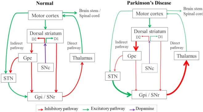
In order to control execution of movements, motor information is modulated by the com-bination of a net excitatory (direct) and inhibitory (indirect) pathway, through basal ganglia structures and cortex, as a closed circuit illustrated in figure 1.1 (left).

Parkinson’s Disease is characterized by progressive degeneration of neurons in SNc, decreasing the secretion of dopamine (DA), an essential brain monoamine which regulates the excitability

(25)

of striatal neurons. Effects of loss of DA lead to alterations in neuronal activity resulting in difficulties for movement control and reflect both in indirect and direct pathways, as represented with thinner arrows in the Parkinson’s circuitry on figure 1.1. Consequently, GPi is hyper-activated and highly increases inhibition signals in the thalamus, finally inhibiting the output to motor cortex and consequently reducing the control of voluntary movements (Maiti et al., 2017).

Figure 1.1: Circuity between basal ganglia-thalamo-cortical motor structures with simplified inhibitory and excitatory connections, in red and green respectively. The left panel indicates the “normal” state, and the right shows the overall changes in activity that have been associated with Parkinson’s Disease. Dopamine from SNc is represented in purple. Thickness of each arrow is representative (directly) with its activity. For simplicity some connections have been omitted from this diagram.

1.1.3 Treatments for Parkinson’s Disease

Different therapies are currently available for the treatment of motor symptoms in PD. At the present, both medication and surgery are the most frequently used therapies to treat PD symptoms, but new promising treatments are emerging and being studied such as stem cell transplantation or gene therapy (Maiti et al., 2017).

During early stages of PD treatment, medication typically is the best option to control motor symptoms. The most commonly used drug is Levodopa (L-dopa) which is a dopaminergic drug that replaces dopaminergic loss associated with SNc degeneration. Nevertheless, since increment of dopamine occurs in other brain regions beyond the basal ganglia, it may generate adverse effects, specially in long-term treatments, such as motor fluctuations or dyskinesias.

(26)

For patients with motor symptoms refractory to medication, different therapeutic approaches can be tried. Surgical approaches include deep brain stimulation and lesion surgery. Lesion surgeries for PD are known as pallidotomy and thalamotomy referring to the respective surgically lesioned part: globus pallidus or thalamus. Motor symptoms decrease with these procedures. It is proposed that the lesions reverse the elevated inhibitory neural activity of these structures. Nevertheless, since lesion surgery is irreversible and lesions in adjacent areas may occur, electrical neuro-stimulation surgery (Deep Brain Stimulation) is a good alternative and currently most commonly used for PD.

1.2 Deep Brain Stimulation

Deep Brain Stimulation (DBS) is a surgical treatment for refractory movement disorders, such as PD, dystonia or tremor. A target area of the brain is stimulated through surgically-implanted electrodes to reverse motor symptoms by inducing neuronal activity alterations.

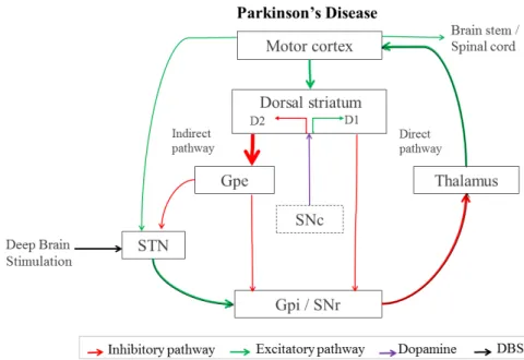
Figure 1.2: Basal ganglia-thalamo-cortical circuitry in Parkinson’s Disease with alterations induced by STN-DBS in both inhibitory and excitatory pathways. Connecting pathways inhibitory (in red), excitatory (in green) and DA from SNc is represented in purple. Thickness of each arrow is representative (directly) with its activity.

Up to 20% of PD patients are considered suitable candidates for Deep Brain Stimulation (DBS), commonly patients in an advanced stage of the disease, with motor fluctuations, and preferentially without psychiatric illnesses (Wagle Shukla & Okun, 2014).

Different proposals on the mechanism underlying STN-DBS were set based on the known basal ganglia circuitry, figure 1.1. However, it still remains fully unclear what mechanisms underlie

(27)

STN-DBS. As illustrated in the basal ganglia neural network in figure 1.2, artificial stimulation in the hyper-activated STN may provoke an inhibition of its firing rate that activates the GPi, consequently inhibiting the thalamus and improving movement control from motor cortex (Maiti et al., 2017; Gradinaru, Mogri, Thompson, Henderson, & Deisseroth, 2009; Negida et al., 2018). The subthalamic nucleus is divided into three functional regions: sensorimotor, limbic and associative, which are located in dorsolateral, anteroventral and medial territories respectively as shown in figure 1.3, and it is part of a bigger functional structure called the basal ganglia as mentioned before. Previous studies suggest that precise positioning of the electrode and stimulation within the sensorimotor part of the STN is of major importance for optimal results and to avoid side effects like mania (Castrioto, Lhommée, Moro, & Krack, 2014; Wodarg et al., 2012; Johnsen, Sunde, Mogensen, & Østergaard, 2010). However, identification of sensorimo-tor STN region based on 1.5 Tesla MRI images is impossible and still unclear based on MER characteristics.

Figure 1.3: Subthalamic Nucleus with functional subdivisions: motor dorsolateral (red), associative medial (blue) and limbic ventro-lateral (yellow) STN. Adapted from Accolla’s atlas.

1.2.1 DBS procedure

Previously to surgery and stereotactic frame implantation, pre-operative MRI is acquired in order to subsequently plan the lead trajectory based on the patient’s anatomy. Pre-implantation contrast-enhanced computed tomography (CT) is performed to the patient, after installation of the stereotactic frame similar to the one in figure 1.4 (right), which displays a reference scale through its ferromagnetic materials.

Estimation of STN target coordinates is based on both CT and MRI pre-operative images co-registered and its STN localization in relation to its fiducial points, anterior commisure (AC) and posterior commisure (PC), as illustrated in 1.4 (left). For both hemispheres (one at a time), different trajectories and strategies are discussed and visualized to achieve the best trajectory based on merged images in both three views (sagital, coronal, axial) and also as probe view, which facilitates avoiding problematic trajectories. The best electrode’s trajectory avoids white matter, critical cerebral tissue, veins or other conflict points.

(28)

Figure 1.4: Fiducial points identified in coronal view anatomic image (left). Stereotactic frame. From Leksell, Elekta.

Once target coordinates are selected, surgery is performed one hemisphere at a time. Stereo-tactic frame is configured according to the target coordinates and after burr hole trepanations, electrodes are connected and implanted into the brain according to the fixed coordinates in the frame.

Registration of microelectrode recordings (MER) is subsequently performed, acquiring neu-ronal activity at different controlled depths along the trajectory to the planned target, as il-lustrated in figure 1.5. Differences in the signal are discernible between different regions of the recorded brain, as neurons present different patterns of spontaneous discharge (Starr, 2002). Recordings used in this study were acquired using 3 channels -central, lateral and anterior- as represented in figure 1.5A. Although up to 5 electrodes (concentrically distributed) are available to use for each lead, they are not commonly used to reduce the risk of complications.

Acquisitions of MER start when electrodes are positioned one centimeter above the planned target, as illustrated in figure 1.5C, and recordings are acquired at different depths simultaneously for all parallel channels. According to the acquired signals and based on intraoperative visual inspection, the region of the brain in which the recording electrode is located, is identified in a table for each recording point. After registration in the different depths and storage for off-line analysis, a reconstruction of the shape of the target is estimated using MER annotations and possible definitive target coordinates are determined/refined.

Intraoperative stimulation is then executed in order to refine the final localization of lead based on therapeutic and side effects assessment. Different estimated points of interest are stimulated through inserted macro-electrodes with gradual variations of both intensities and frequency. Once stimulation induced side effects, such as eye or muscle contractions, are assessed and the best position is determined, definitive electrode is implanted.

The second part of surgery includes the implementation of the neurostimulator with the bat-tery in the patient and its connection to the electrodes as illustrated in figure 1.6 from Medtronic

(29)

Figure 1.5: Position of the channels for intraoperative microelectrode recordings (A). Trajectory of the lead to STN with subdivisions and GPi in green, GPe in blue and thalamus in yellow. Lateral and anterior channels illustrated as grey lines (B). MER signals recorded through the trajectory with center, lateral and anterior electrodes. Recordings presumably from STN are identified within the grey box. Segments of MERs (500 ms duration) with central channel at each depth along the trajectory with central electrode, starting recordings from 10 mm above target to 3.5 mm under (C).

(2007). Both rechargeable and not rechargeable stimulators are available on the market for DBS. Rechargeable batteries may last between 9 and 25 years whereas non-rechargeable batteries may need to be replaced in 3 to 5 years depending on the patient and stimulation parameters (Hariz, 2017).

Figure 1.6: Illustration of basic implanted components of the DBS System Components: lead, extension, neurostimulator and pocket adaptor. From Medtronic.

(30)

(31)

Chapter 2

Objectives

Clinical-support tools for identification of the target area in DBS are necessary in the field. As mentioned before, positioning the final electrodes in the precise location has a vital role in obtaining the best therapeutic results. However, this decision depends on the expertise of the intra-operative evaluation performed by the neurologist, making it a time-consuming and subjective process.

In this study we intend to contribute to the development of computational tools that can assist target identification in STN-DBS. We split our objective into four main tasks:

1. Identification of features based on time and frequency domain to distinguish STN from non-STN intraoperative MER. Development of an unbiased unsupervised tool for extraction of these MER features through loading, preprocessing and analysis, but easily adaptable for other types of signals and regions.

2. Development of an automatic approach for spike sorting and signal analysis of human brain MER. Through this tool, features related with neuronal activity are studied to find relevant characteristics for STN identification. We aim to construct this tool generalizable to other brain regions and unsupervised through the adjustment of existing algorithms to our approach.

3. Development of a hybrid unsupervised/supervised machine learning classification approach that uses extracted MER features based on time and frequency domain for high-accuracy identification of STN.

4. Identification of features that distinguish sensorimotor subdivision of STN vs. limbic and associative using extracted features from both previously constructed tools. This approach can be optimized using individual patient lead trajectory localization reconstruction based on imagiology, fused with an STN functional subdivision atlas.

(32)

(33)

Chapter 3

Methods

In the present chapter, we describe the dataset used in the analysis. Then, procedures for labelling each MER regarding its position within the target area of the brain are detailed followed by the pre-processing approaches for MER to clean the signals. Methods for extraction of features, both directly from signal and from neuro-physiological information, are described in sections 3.5 and 3.4.

3.1 Microelectrode recordings (MER) dataset

Our database was collected from 5 PD patients undergoing bilateral STN-DBS. Three registry electrodes were used in each hemisphere and the lateral and anterior channels were positioned 2 mm from the central one (impedance of each microelectrode is 1 MΩ ± 20% at 1000 Hz). Recordings started 10 mm above the estimated target and ended approximately 3.5 mm after, thus signals were acquired at around 23 different depths in each channel, as shown in figure 1.5. Acquisitions were obtained through a MER system (Medtronic, Minnesota, MN, USA), sampled at 24 kHz per channel, filtered (band-pass filtering, 0.5-5 kHz) and amplified (with total gain of 1000), previously to their storage. Signal was recorded during 10 seconds for 3 patients, and 30 seconds for 2 patients and analysis were performed on 10 seconds duration MER segments.

3.2 Localization of MER position

Labelling each MER of our dataset regarding its position is important to effectively identify fea-tures distinguishing STN and non-STN MER and to construct the automatic classifier. Therefore, different approaches are explored for labelling MER regarding its location within the target, both further explained in the following sections.

(34)

Expert based classification was used in previous studies using 1) intraoperative annotations based on visual inspection during recording phase of DBS surgery, 2) off-line MER labelling or 3) other expert-based approaches (Cagnan et al., 2011; He, 2009; Bakštein et al., 2015). Nevertheless, expert classification as STN vs. non-STN based on visual inspection may be biased by previous geometric knowledge of the MER trajectories and/or estimated target area. Therefore, we approached this issue trying to reduce the bias with offline labelling of MER segments using random order.

Ongoing work is refining the labelling, making it based on lead trajectory localization recon-struction using individual patient imagiology, fused with an STN functional subdivision atlas. Gold-standard classification could be obtained through this approach and it allows us to com-pare physiological neurons properties in motor/non-motor STN and it is further explained in section 3.2.2.

3.2.1 Expert-based classification

Labels regarding each signal’s position within the brain (STN/non-STN) were identified through visual inspection by an expert as previously referenced. In order to facilitate visualization and labelling of all signals and to preserve the classification unbiased to knowledge about MER depths, a customized script in Matlab was programmed.

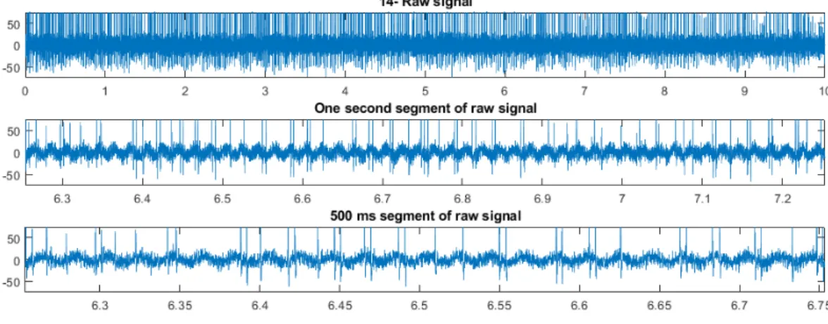
Figure 3.1: Segments of MERs (1 s and 500 ms duration) and raw signal shown for classification by the expert through visual inspection.

This script first shuffles all signals in the dataset and it plots in random order one signal at a time. The whole signal and two enlarged segments (1 second and 500 milliseconds duration, randomly chosen from the raw signal) are presented for classification, as shown in figure 3.1 for each signal in the dataset. Then, the expert is asked to identify the current signal as STN (1), not-STN (2) or try again (3). If any signal is classified as try again for the first time, it is shown again until the third attempt, when it is classified as unclear (3). Additionally for each signal

(35)

classified as STN, the expert is asked to set its value of certainty of its localization from 1 (very unclear) to 5 (high certainty), which gives an idea of the confidence of each classification for further analysis.

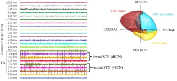
However, labelling subterritories of STN based on visual inspection is not an optimal option since differences are not clearly known or visually recognizable on MER. Accordingly, to explore if preliminary differences may be present between STN subregions, this subdivision is manually defined on the consecutive previously labelled MER. Previously defined STN recordings were split in two parts: dorsal and ventral STN, for the shallower and deeper depths labelled as STN respectively as illustrated in figure 3.2. Additionally, MER classified as STN located between both deep and shallow regions are discarded, resulting in labels for both dorsal and ventral regions, with a higher probability of being motor and non-motor STN respectively.

Figure 3.2: Segments of MER at different depths with STN expert identification and its subdivision on dorsal and ventral STN.

3.2.2 Anatomically-based classification

Reconstruction of trajectory localization for each lead presents a gold-standard approach, since it is based on both pre-operative and post-operative patient’s imagiology fused to an atlas of STN functional subterritories. Ongoing analysis to localize MER based on the reconstructed electrode tip and its trajectory with patient’s image processing was performed with LeadDBS, a Matlab toolbox [http://www.lead-dbs.org; (Horn & Kühn, 2015)]. Along with Slicer3D [https://www.slicer.org/], used to import all provided Digital Imaging and Communications in Medicine (DICOM) images into Nifti, which is the default file format in the used packages. Nifti stands for Neuroimaging Informatics Technology Initiative and it is a medical image file format created to simplify post-processing analysis (Larobina & Murino, 2014).

(36)

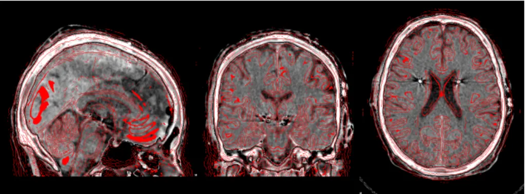
First, registration of all pre- and post-operative images is performed, which consists in the geometric alignment of these images between each other through transformations to allow their fusion. Therefore and through Lead DBS, MRI images are coregistered using Statistical Para-metric Mapping 12 (SPM12) method [http://www.fil.ion.ucl.ac.uk/spm/software/spm12/], whereas post-operative contrast-enhanced CT image was coregistered to preoperative MRI im-ages with Advanced Normalization Tools (ANTs) [http://stnava.github.io/ANTs/].

Figure 3.3: Normalization of post-operative CT to the MNI2009b space, previously registered to pre-operative MRIs.

Normalization is then performed to transform the previous volumes to a known space in which we will superpose an atlas. Consequently, all volumes are normalized to standard stereotactic MNI space (ICBM152 2009b non-linear asymmetric) using Diffeomorphic Anatomical Registra-tion Through Exponentiated Lie algebra (DARTEL) implemented in SPM12 (Friston, Ashburner, Kiebel, Nichols, & Penny, 2006).

After coregistration and normalization, subcortical refinement of previous transforms is per-formed to correct brainshift, which may happen during surgery when the skull is opened and air gets inside, moving the brain in respect to the skull. We applied this process through Lead-DBS using specific masks from Schönecker, Kupsch, Kühn, Schneider, and Hoffmann (2009) in 2 patients, to estimate a transform for refinement of the overlapping in subcortical regions, as illustrated in figure 3.4.

In order to obtain electrode’s location and trajectory, reconstruction is manually supervised assessed with pre-reconstruction through Precise and Convenient Electrode Reconstruction for Deep Brain Stimulation (PaCER) method and Acolla’s STN subterritories atlas (Accolla et al., 2014; Husch, Petersen, Gemmar, Goncalves, & Hertel, 2018), as illustrated in figure 3.5.

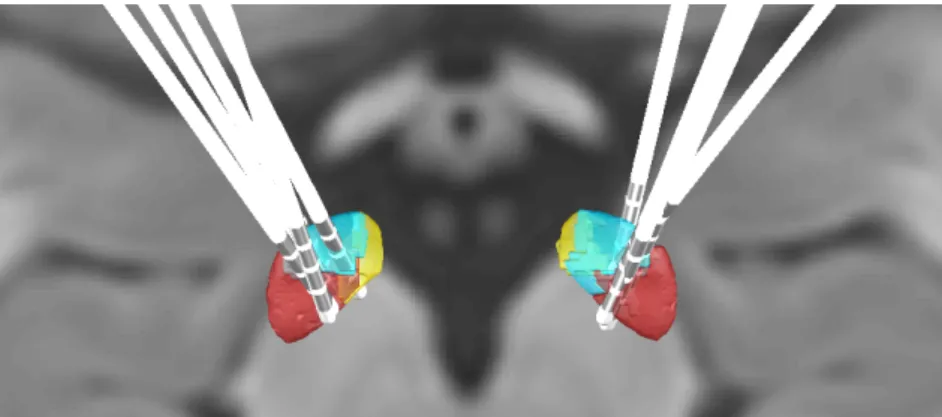
Once definitive coordinates of electrode are located, MER localizer tool in LeadDBS is used to determinate locations along the trajectory in the selected channels in relation to the STN-subdivisions atlas, as shown in figure 4.2 where each yellow ball represents the location of each introduced recording site. This step is currently ongoing, therefore only data from patient 4 (which presented the majority of STN located MER according to the expert labelling) is presented in the results for STN subterritories refinement, in section 4.5. However, all patient’s trajectories

(37)

Figure 3.4: Application area for masks (Schönecker et al., 2009) (left) and results of subcortical refine-ment on normalized images (right).

Figure 3.5: Lead reconstruction interface with Lead DBS using PaCER.

have been reconstructed, as illustrated in figure 3.6.

Figure 3.6: Axial view of STN subdivisions with reconstructed electrodes based on each patient’s images through Lead DBS.

(38)

3.3 MER filtering and artifact detection

Noisy signals are present in MER dataset with different types of artifacts. According to Bakštein et al. (2017), noise in MER may affect more than 25% of the recording length and can arise due to a number of factors such as mechanical movement manifested by high power signal peaks, electromagnetic interference such as the 50 Hz interference from the power grid, low-frequency interferences (<50 Hz) and "irritated neurons" with high spiking activity. Consequently, pre-processing these signals is an important step to avoid errors in the extracted features and obtain better accuracy results in classification.

Figure 3.7: Filtered signal (150 ms) with elliptical band pass filter (green) overlapped to raw MER (grey) presenting low-frequency interference.

Filtering the signal is our first step in this pre-processing part, since it can smooth out high-frequency fluctuations and/or remove periodic trends of a specific frequency from data. Therefore, we filter the data using an elliptic band-pass filter between 300 and 5000 Hz. Elliptic filter was chosen after visual inspection of different types of filters (Butterworth and Chebyshev type II) and its effects on spike detection, since it keeps waveforms of firing neurons unaltered (Quiroga, 2009). Implemented filter of order 4 is set to 0.6 decibels (dB) of peak-to-peak ripple and 60 dB of attenuation and it is performed with zero-phase digital filtering in order to preserve time features. Nevertheless, all parameters can be easily modified in our tool and code for testing other types of filters is implemented.

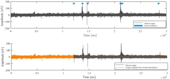
In addition to the filtering, we reviewed previous approaches for MER artifact removal litera-ture and visually inspected their performances on our dataset (O’Shea & Shenoy, 2017; Bakštein et al., 2017, 2015; Grubhoffer, 2016). Best observed approach for artifact detection was found using the autocorrelation-based method as implemented by Bakštein et al. (2015), but this algo-rithm was actually previously developed by Aboy and Falkenberg (2006). We adapted Bakštein et al.’s open-source code to extract the longest consecutive clean segment from signal used for

(39)

extraction of neuronal activity features, as illustrated in figure 3.8.

Figure 3.8: Artifacts detection. Filtered signal with detected noisy segments in blue (Top). Longest clean segment free of detected artifacts in orange (Bottom).

3.4 Extraction of features related with time, frequency and noise

As previously described, differences between raw signals along the trajectory to target are dis-cernible through visual inspection. Therefore signal characteristics calculated through compu-tational analysis might reflect these variations. In line with this, features related with time, frequency and noise are extracted from filtered MER to find features for distinguishing STN from non-STN recordings.

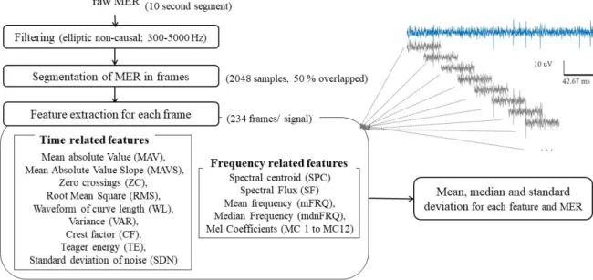
In order to identify STN, custom Matlab code was developed for MER analysis. After setting input parameters, the analysis was done in an unsupervised way, following steps presented in figure 3.9. Each raw signal is first filtered as explained in section 3.3 followed by artifact detection, in order to obtain segments free of artifacts.

Filtered signal is divided in smaller segments with Hanning windows of 2048 samples over-lapped 50% (1024 samples), resulting in more than 230 segments for each used segment for analysis of 10 second (sampled at 24 kHz). Characteristics are computed for all frames indepen-dently and then statistics (mean, median and standard deviation) are stored for each MER using all segment’s values. This division in frames should provide a more robust approach for signals with noisy segments or high variability within the same signal vs. extraction of characteristics from the whole signal.

(40)

Figure 3.9: Workflow for MER analysis and extraction of time and frequency related features.

value (MAV), mean absolute value slope (MAVS), zero crossings (ZC), root mean square (RMS), waveform of curve length (WL), Teager energy (TE), variance (VAR) crest factor (CF). In relation to noise, an estimation of the standard deviation of noise (SDN) was obtained ac-cording to Dolan, Martens, Schuurman, and Bour (2009). Features related with frequency do-main are: spectral centroid (SPC), spectral flux (SF), mean frequency (mFRQ), median fre-quency (mdnFRQ) and 12 Mel-frefre-quency cepstral coefficients (MC). We selected this set of features related with time and frequency based on a preliminary study through the related liter-ature for STN identification, MER analysis and typical feliter-atures used in other signal processing fields such as sound processing (e.g. Mel Coefficients) and further definitions of these features are presented in appendix A.

3.5 Features related with neuronal activity

Microelectrodes register neuronal activity, part of which consists on action potentials (APs), spikes generated from neurons in the nearest region of the electrode tip. Because there are dif-ferent structures with difdif-ferent functional and cellular density across the lead trajectory, MER of the brain show different neuronal activity. In addition, activity of more than one different neuron near the recording tip can be registered, but spikes from the same neuron present similar shapes and amplitudes in each MER. Consequently, prior to the spike-related features quantification, identification of the different neurons from each recording is important to obtain reliable features. Action potentials of the different neurons are detected from the MER as spiking events by a process known as spike detection, further explained in section 3.5.1. After storage and

(41)

alignment of the detected spikes to their maximum, different neurons are separated in different clusters, process detailed in section 3.5.3 and known as spike sorting. Extraction of their features is implemented lastly, once neurons are sorted and detected from each MER. This sequence of steps for signal processing and neuronal characteristics is illustrated in the diagram in figure 3.10.

Figure 3.10: Workflow process for neuronal activity analysis and extraction of spike related features.

3.5.1 Spike detection

In this process, firing neurons are detected as spike events from the filtered signal. The chosen algorithm is Spike Detection with Continuous Wavelet Transform (Nenadic & Burdick, 2005). This algorithm uses the continuous wavelet transform (CWT) combined with information about the typical interval duration of APs to identify these spiking events. Biorthogonal family was used with this algorithm, though it can be used with other types of wavelets, but this family presents bi-phasic phase which is similar to the brain’s action potentials and when translated and scaled, a bank of approximately matched filters for APs identification along the signal is formed.

Nenadic and Burdick’s algorithm (2005) was chosen instead of threshold detection, the most commonly used method in related studies, since it presented better performance with an un-supervised approach on the number of detected spikes, particularly in noisy signals. This may be due to the fact that this method is less affected by the high variability of amplitudes and background noise between all signals and more stable for unsupervised analysis.

(42)

Figure 3.11: Spike train of detected spike events (red) on the clean filtered signal (grey).

3.5.2 Spike alignment

Once spikes are detected, further analysis is needed to store the spikes and sort them according to their neuron of origin, since as mentioned before detected spikes from one signal are probably provoked by more than one different neuron. Nevertheless, the maximum local value of the spike segment could appear on different samples and this miss-alignment may affect the spike sorting process. Therefore, previously to their sorting, a segment of 22 samples before the sample of the detected spike to 26 samples after is stored. Afterwards, cubic spline interpolation is performed to interpolate a curve with 10 times as many points which goes through the same original samples of the spike segment. Then, spikes segments are aligned to their local maximum and extrapolation is performed and the segment is cropped to 1.5 ms (16 samples before the maximum, 20 samples after) and stored for further analysis.

3.5.3 Spike sorting

Detected firing events within the same signal may be originated from more than one different neuron. Consequently, it is important to correctly identify their origin to avoid misclassifications and errors in the spike related features. Spike sorting consists in grouping the detected spikes into clusters based on the similarity of their waveforms.

Since we aim to develop an unsupervised tool for neurophysiological features extraction based on MER, we research the spike sorting literature to find a suitable algorithm to adapt to our anal-ysis tool. Our spike sorting is performed with linear discriminant analanal-ysis (LDA), gaussian mix-ture model (GMM) and outlier detection, through an available algorithm and implemented code in Matlab from Keshtkaran and Yang (2017). This method performs clustering with subspace

(43)

learning using LDA, which is a linear transformation technique commonly used for dimensionality reduction, to extract most discriminative features from the spike waveforms. Automatic initial estimation of the number of the clusters is based on GMM, a clustering models that adapts to spherical clusters and facilitates implementation of outlier detection, as explained by the authors.

Figure 3.12: Detected spikes in filtered MER after spike detection and sorting (top) and their respective overlapped waveforms (bottom).

To address the quality of each cluster in an objective and standardized way, different related measures are extracted through existing algorithms. Regarding the isolation quality for each cluster, isolation score (IS) is quantified as explained in Joshua, Elias, Levine, and Bergman (2007). This score measures the overlap between the noise and the spike clusters. Also with the same algorithm, an estimation of the proportion of false positive (FP) and false negative (FN) classification errors is obtained.

3.5.4 Spike related features extraction

Different groups of characteristics were studied from the related literature on the field to select features that could provide relevant information for distinguishing STN and non-STN MER. We’ve extracted features related with the periodicity of each spike train, which is a binary vector with 1 where each neuron’s spike event occurs. Features related with the bursting activity for each spike train were also calculated among other spike characteristics. In total, 15 spike related features were extracted through custom Matlab code and also 3 quality measures as explained before. Spike related features are presented following, but further definitions of these features are available in appendix A.

Quantification of the variability of the increments of a spike train is measured through the fano factor (FF), calculated according to the literature (Kuebler & Thivierge, 2014). Median values of spike peak-to-peak amplitude (SppA) are also stored as measurements of spikes events

(44)

amplitude, and firing rate (FR) is extracted as a measure of the number of spikes per unit. A group of features is based on periodicity of the spike trains, specifically related with the interspike interval (ISI). These features are pause index (PI), pause ratio (PR), assimetry in-dex (AI), median interspike interval (mdnISI), standard deviation of interspike interval (stdISI) and coefficient of variation of interspike interval (cvISI). Features for an estimation of burst-ing activity directly obtained from ISI are modified burst index (MBI) and burst index (BI) (Rajpurohit, Danish, Hargreaves, & Wong, 2015).

Nevertheless, characteristics related with bursting neurons are further calculated after bursts are previously detected through the Rank Surprise algorithm (RSA), which is again based on ISI for detecting bursts (Gourévitch & Eggermont, 2007). Extracted features from bursting neurons are: burst rate (BR), median interburst interval (mdnIBI), median burst duration (mdnBD), median intraburst frequency (mdnIBF).

3.6 Statistics

Statistical comparison of STN and non-STN regions based on MER features was computed through different statistical approaches. Considering independent signals, Student’s T-test, a parametric test, was performed in samples with size equal or bigger than 30 or otherwise when following a normal distribution, according to Lilliefors test combined with visual inspection of histograms. Non-parametric Mann Whitney U test, also known as Wilcoxon rank sum test, was used in non-normal distributed features when the sample size is less than 30. Results were considered statistically significant for an α value equal to 0.05.

Random Permutations test (also known as randomization test) was also used to compare features across STN motor vs. non-motor in spike related features to verify the results obtained through the previous method. It is a non-parametric test which doesn’t make assumptions about the data through the permutations of the values. Therefore, data from both samples was shuffled 100000 times, creating a reference distribution for the difference in means between the two samples, which is the observed value. Features are considered statistically different across compared regions if the observed value lies outside the confidence intervals of the reference distribution (again for α = 0.05).

3.7 Classification with Machine Learning

Automatic identification of the signals recorded in the interest area was performed through classification with machine learning techniques. We’ve used previously extracted features related with time and frequency combined with the information of the electrode’s localization along the trajectory. Classification consists in the categorization of an observation to a class or group

(45)

based on previous extracted features or characteristics and their respective labels through pattern recognition machine learning models.

This is a supervised approach since the algorithm needs to learn with a known set of labelled data in order to make predictions. Nevertheless, feature extraction and reduction is performed in an unsupervised manner.

Improvement in accuracy is found when the volume of training data is increased. Before training the model, the classification algorithm is projected and selected through exploration of prediction accuracy measurements. Once the selected algorithm is trained, test data is classified with the trained model and validation is performed to test the performance of our classifier and its capability of generalization.

Multiple models are available for classification of data such as decision trees, discriminant analysis, nearest neighbour classifiers, logistic regression classifiers or support vector machines among others. Since our data has two classes (STN and non-STN) and a set of features with no categorical values and due to its versatility through the use of different kernel functions, support vector machine (SVM) was chosen for the classification procedure as explained in next section, which uses a subset of points in the decision function, reducing memory usage, although further analysis are planned with different models as future work.

3.7.1 Support Vector Machine

Support vector machine classifies data into different classes by finding a hyperplane in an N-dimensional space (where N is the number of features) with the largest margin to separate both classes. Support vector are the data points that are closest to the hyperplane and influence its position and orientation, since the margin to maximize refers to the distance between the hyperplane and the support vectors (Cortes & Vapnik, 1995).

Data points from different classes may be separable linearly with the hyperplane, which is the SVM approach by definition. Nevertheless, if data is linearly non-separable, non-linear alterna-tives of SVM are available through the use of kernel functions. Data points are transformed to a higher dimension in order to separate classes using a hyperplane. Further information regarding SVM and kernels is available in literature (Hu, 2000; Cortes & Vapnik, 1995).

In the present study, 4 kernel functions are trained and tested along with the linear approach: quadratic, cubic, and 3 types of gaussian kernel (fine, medium and coarse), also known as radial basis function.

3.7.2 Cross validation

Standard approach for prediction of accuracy of the trained model is cross-validation and in par-ticular k-fold cross validation is commonly used. This procedure consists on randomly splitting

(46)

our data in a number of folds (k), then for each fold, the model is trained using the out-of-fold observations and tested with the present fold. Evaluation of the classifier performance is mea-sured through an estimated average test error with the results over all folds. Validation using 10-cross validation (CV) was performed through the Classification Learner App in Matlab, to explore algorithm’s performance and visualize features in a fast and simple way.

Nevertheless, as explained in Little et al. (2017), the correct methodology for validation of a classifier with patient’s observations is leave-one-subject out cross validation to ensure that features from patient for test has never seen the trained model. Leave-one-out cross validation is a specific case of k-fold validation where k is equal to the number of observations. Additionally, in our approach of leave-one-subject-out cross-validation, folds are not randomly chosen, but defined by patient identification. Therefore, for each iteration or validation, one patient is excluded from the training data and used for testing the trained model, as illustrated in figure 3.13. Since this approach is not available on the Classification Learner app, we trained, tested and validated our classifier through custom code for preparation of data, classification and error estimation.

Figure 3.13: Cross-validation iterations for leave one subject out approach

3.7.3 Feature reduction

To reduce the dimension of the sample, feature reduction is performed through principal com-ponents analysis (PCA) combined with SVM as in previous studies (Guo et al., 2016; Sahak, Mansor, Lee, Yassin, & Zabidi, 2010). Original features are projected into a linear space of lower dimensionality, defined by the PCA principal components (PCs). Since this PCs are orthogonal to each other, redundant information and correlation from the original features is discarded.

(47)

3.7.4 Classification performance measurements

Evaluation of classification performance is assessed through four indicators: accuracy, specificity, sensitivity and precision.These indicators are calculated based on the prediction values from the confusion matrix for each model as indicated in figure 3.1, where true positives (TP) is the number of true positive predictions, false positive (FP) the incorrect positive prediction and true negatives (TN) and false negative (FN) are consequently the correct and incorrect negative predictions. Accuracy represents the proportion of the number of correct predictions, whereas sensitivity or recall and specificity represent the proportions of positives (STN) and negatives (not-STN) correctly classified, respectively. Additionally, precision is the portion of correctly classified as positives from all positives.

Table 3.1: Confusion matrix and its evaluation measures, where TP represents the number of true positives, FN as false negatives, FP is false positives and TN true negatives.

Target

Confusion matrix Positive Negative

Model Positive TP FN Sensitivity TP/(TP+FN) Negative FP TN Specificity TN/(TN+FP)

Precision

(48)

(49)

Chapter 4

Results

In the present chapter results are presented following the same order as the stated objectives, except for section 4.1 which first presents characteristics of our set of MER and their expert-based classification as STN or not.

4.1 MER dataset

Our set of MER is composed by 702 intraoperative MER during STN-DBS, from 5 patients, each with 2 hemispheres and 3 channels or electrodes recording simultaneously and in parallel through its trajectory, which changes depending on the patient as illustrated in table 4.1, between 21 to 27 depths for each hemisphere.

Table 4.1: Characteristics of subjects, recording duration and number of MER depths. UPDRS III represents the motor evaluation of Unified PD Rating Scale for each subject, scored through a structured neurological examination (range between 0 and 108). Gender indicated as female (F) and male (M).

Age at surgery (years) Disease duration at surgery (years) UPDRS III score

Intraoperative MER characteristics

Patient Gender Duration

(seconds)

Depths along trajectory to target

Right Hemisphere Left Hemisphere

1 M 61 10 66 30 21 21

2 M 67 12 83 10 25 24

3 M 54 13 36 10 27 25

4 M 67 10 57 30 22 23

5 F 37 5 32 10 24 23

4.1.1 Expert labels and STN subdivision

Identification of MER localizations was performed based on visual inspection of the randomized dataset by an expert as explained in section 3.2.1. STN was identified in 285 recordings in

(50)

our dataset of 705 MER signals and detailed results and certainty of STN classification are illustrated in table 4.2. Number of STN vs. non-STN labels and certainty of MER classification as STN varies between patients, e.g. 38 recordings were labelled with the maximum certainty levels (>95%) in patient 4, whereas in patient 3 no MER was identified as STN maximum certainty. This may be due to multiple reasons: differences in trajectories between patients and hemispheres, the electrode is actually not recording along the STN with the chosen trajectory or miss-classifications in the visual inspection labelling, which could be further explored with the gold-standard approach.

Table 4.2: Results of expert based classification of MER by visual inspection. Number and percentages of MER labelled as STN, not-STN and total per patient and for all patients. Number of recordings for each certainty level labelled as STN.

Number of MER non-STN STN Certainty Total Total <25% 25-50% 50-75% 75-95% >95% All patients 705 420 (59.6%) 285 (40.4%) 70 60 36 66 53 Patient 1 126 (17.9%) 58 (46.0%) 68 (54.0%) 10 14 16 19 9 Patient 2 147 (20.9%) 122 (83.0%) 25 (17.0%) 9 4 5 5 2 Patient 3 156 (22.1%) 113 (72.4%) 43 (27.6%) 14 25 3 1 0 Patient 4 135 (19.1%) 39 (28.9%) 96 (71.1%) 14 9 6 29 38 Patient 5 141 (20.0%) 88 (62.4%) 53 (37.6%) 23 8 6 12 4

The following results were computed considering STN-MER when the certainty level set is higher than 50%, and discarding signals with the lowest certainty levels. Therefore, 155 record-ings are considered from the STN, which represents approximately 22% of the whole sample, almost 55% of the total recordings initially labelled as STN.

Regarding STN subdivisions (dorsal vs. ventral) manually defined on STN labelled for the results in section 4.5, we visualized these 155 STN-labelled recordings with maximum certainty and divide them in relation to its depth. Consequently 73 signals were considered as dorsal subthalamic nucleus (dSTN) and 74 as ventral subthalamic nucleus (vSTN), excluding 8 MER spatially located in the presumed frontier between dSTN and vSTN according to their depth.

4.2 Features related with time and frequency

Differences in extracted features were studied for distinguishing STN from non-STN MER from our dataset through our developed code.

To automatize the process of feature extraction with previous loading and preprocessing of MER, Matlab code was developed which can be generalizable for other types of recordings. Since our approach computes features from each signal based on small segments of the signal, we expected artifacts not to influence very significantly our results. Therefore, first analysis of extracted features for distinguishing STN and non-STN recordings using this tool was performed