Climate change policy in Brazil and Mexico: Results from the MIT
EPPA model
Claudia Octaviano
a,⁎
, Sergey Paltsev
a, Angelo Costa Gurgel
a,ba
Joint Program on the Science and Policy of Global Change, Massachusetts Institute of Technology, USA bSao Paulo School of Economics, Fundacao Getulio Vargas, Sao Paulo, Brazil
a b s t r a c t
a r t i c l e i n f o
Article history: Received 26 August 2014
Received in revised form 23 March 2015 Accepted 13 April 2015
Available online 22 April 2015
JEL classification: C61 D58 Q43 Keywords: Climate policy Brazil Mexico General equilibrium Land use Biofuels
Based on an in-depth analysis of results from the MIT Economic Projection and Policy Analysis (EPPA) model of climate policies for Brazil and Mexico, we demonstrate that commitments by Mexico and Brazil for 2020—made during the UN climate meetings in Copenhagen and Cancun—are reachable, but they come at different costs for each country. Wefind that Brazil's commitments will be met through reduced deforestation, and at no additional cost; however, Mexico's pledges will cost 4 billion US dollars in terms of reduced GDP in 2020. We explore short-and long-term implications of several policy scenarios after 2020, considering current policy debates in both countries. The comparative analysis of these two economies underscores the need for climate policy designed for the specific characteristics of each country, accounting for variables such as natural resources and current eco-nomic structure. Our results also suggest that both Brazil and Mexico may face other environmental and econom-ic impacts from stringent global climate poleconom-icies, affecting variables such as the value of energy resources in international trade.
© 2015 The Authors. Published by Elsevier B.V. This is an open access article under the CC BY-NC-ND license (http://creativecommons.org/licenses/by-nc-nd/4.0/).
1. Introduction
In the context of climate change mitigation policy, larger developing countries will play an important role in future long-term international agreements. Brazil and Mexico are both upper-middle income coun-tries, with higher income per capita—$11,690 and $9940 US dollars, respectively—than the average in Latin America ($9314 US dollars) (WB, 2014). There are 200.4 million people in Brazil, and 120.8 million people in Mexico (UN, 2013); together, they account for 55% of the Latin American population. In 2012, with GDPs of $2.25 trillion (Brazil) and $1.18 trillion (Mexico), together they represented 62% of the Latin American economy (WB, 2014). As the biggest economies in Latin America, Brazil and Mexico play a central role in climate change mitiga-tion, and have been under significant international pressure to enhance mitigation action. Both have actively participated in international miti-gation efforts under the UN Framework Convention on Climate Change (UN, 2009, 2010), as well as in other policy forums such as the G8+5 Climate Change Dialogue. While Brazil and Mexico's emissions are not among the largest in the world, their contributions to GHG emission
mitigation are extremely important for several reasons. To reach reduc-tions substantial enough to eliminate the worst potential consequences of future climate change, all countries must participate in mitigation ef-forts (IPCC, 2014); Brazil and Mexico are key leaders among middle-income countries, and can help to engage the developing world in cli-mate negotiation processes.
In 2005, Brazil and Mexico emitted 2032 and 667 million tonnes (Mt) of CO2e respectively (MME and EPE, 2013; SEMARNAT, 2013).1
By 2010, Brazil had reduced emissions by 39%, to 1246 million tonnes CO2e (6.8 tonnes per capita) with 2.2 tonnes CO2per capita from energy
alone. A recent deforestation control policy contributed to this change—land-use emissions dropped sharply, resulting in a net emission reduction despite the continued upward trend of industrial and agricultural emissions. In the same period, Mexico's emissions in-creased by 12%, to 748 million tonnes CO2e (6.1 tonnes per capita)
with 3.8 tonnes CO2per capita emissions just from energy.
Brazil and Mexico are both signatories of the UNFCCC and its Kyoto Protocol, and as active members of the ongoing UN climate negotiations, they have both implemented national strategies for climate change
⁎ Corresponding author at: Joint Program on the Science and Policy of Global Change, 77 Massachusetts Ave., Cambridge, MA 02139, USA. Tel.: +1 617 253 7492.
E-mail addresses:[email protected](C. Octaviano),[email protected](S. Paltsev),
[email protected](A.C. Gurgel).
1
Thesefigures include emissions from fossil fuel use, other industrial emissions and land use change.
http://dx.doi.org/10.1016/j.eneco.2015.04.007
mitigation. Key strategies implemented by Brazil include deforestation control programs and policies targeting the development of renewable energy. Mexico has also made remarkable progress using strategies in-cluding the implementation of a carbon tax, programs promoting re-newable energy and energy efficiency, and deforestation control strategies.2
As UNFCCC members prepare their positions and policies for the post-Kyoto world, studies that provide insights regarding comparative mitigation efforts between peer countries are likely to be useful during climate negotiations. The goal of this paper is to compare options for GHG reductions in Brazil and Mexico, and to explore similarities and dif-ferences in their potential approaches to climate change mitigation. We seek to understand if a global“one-size-fits-all” policy (e.g., identical carbon price or emission reduction percentages) can be justified, or if the countries should focus on their own strategies for emission mitiga-tion. We use the MIT Economic Projection and Policy Analysis (EPPA) model (Paltsev et al., 2005), a global energy-economic computable gen-eral equilibrium (CGE) model developed at the MIT Joint Program on the Science and Policy of Global Change. The scenarios were developed by the Latin America Modeling Project and the Integrated Climate Modeling and Capacity Building Project in Latin America (LAMP/ CLIMACAP) described in detail invan der Zwaan et al. (2016a)in this Special Issue. In this paper we mostly focus on the results from the EPPA model and provide some comparisons with the other model par-ticipated in the LAMP/CLIMACAP project.
We focus on the dynamics of emission trends, analyze resulting en-ergy choices and explain the macroeconomic costs in climate policy sce-narios. The paper is organized as follows.Section 2describes the EPPA model.Section 3provides an overview of the reference scenario, detail-ing the emissions, energy and electricity mix in the business-as-usual case, and describing some of the key differences in energy structures af-fecting policy costs.Section 4presents the results of several climate pol-icy scenarios.Section 5concludes.
2. The MIT EPPA model
The EPPA model is a multi-region, multi-sector recursive dynamic representation of the global economy (Paltsev et al., 2005). The GTAP data set provides the base information on the input–output structure for regional economies, including bilateral tradeflows (Dimaranan and McDougall, 2002; Hertel, 1997). We aggregate the data into 16 regions and 21 sectors. The base year for the model is 2005, based on the calibra-tion of the GTAP data for 2004, and from 2005 the model solves at 5-year intervals. We also further calibrate the data for 2010 as described later.
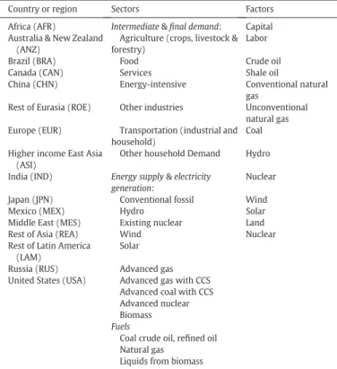
Table 1presents the countries (or regions) represented in the model, broadly identifying Intermediate and Final Demand sectors and Energy Supply and Conversion sectors. Energy Supply and Conversion sectors are modeled in sufficient detail to identify fuels and technologies with different GHG emissions and to represent both fossil and non-fossil ad-vanced technologies. There are 16 geographical regions represented ex-plicitly in the model, including 8 major countries (Brazil, Mexico, USA, Japan, Canada, China, India and Russia) and 8 regional aggregations of other countries. For the CLIMACAP/LAMP modeling exercise, all regions were modeled as specified in EPPA, but in this paper we only report re-sults for Brazil and Mexico.
The production structure for electricity is the most detailed of all sec-tors, and captures technological changes that will be important to track under climate policy (Fig. 1). The top-level nests allow different treat-ments for traditional and advanced generation technologies (conven-tional fossil, nuclear, and hydro, natural gas and coal CCS, IGCC, advanced combined cycle technologies, bioelectricity, wind and solar).
Most of the advanced technologies enter as perfect substitutes for existing technologies (i.e., the elasticity of substitution is infinite), ex-cept for renewable energy technologies, which have a special treatment in the model. We represent two types of penetration for wind and solar technologies. At low levels of penetration, generic wind and solar tech-nologies are modeled as producing an imperfect substitute of electricity, reflecting diurnal and seasonal variability and intermittency. At large-scale penetration, we allow wind and solar to enter as perfect substi-tutes, but require a back-up generating unit either from natural gas or biomass. We introduce these as“hybrid” technologies, as wind and solar technologies will require additional capacity to overcome inter-mittency issues before they can be competitive under climate policy. Biomass use—where a liquid fuel is produced and assumed to be a per-fect substitute for refined oil—is included both in electricity generation and transport.
The deployment of advanced technologies is endogenous to the model. Advanced technologies, such as cellulosic biofuel or wind and solar technologies, enter the market when they become cost competi-tive with existing technologies. Technologies are ranked according to their levelized cost of electricity (EIA, 2014), plus additional integration costs for wind and solar (Morris et al., 2010). When a carbon price ex-ists, low carbon technologies are introduced as explained by
McFarland et al. (2004). Initially, afixed factor is required to represent costs of deployment (e.g. institutional costs, learning costs) for new technologies that—while competitive—require some time to penetrate into the market. Thefixed-factor supply grows each period as a function of deployment until it becomes non-binding, allowing for large-scale deployment of the new technology. A complete description of the nesting structure of electricity generation in the EPPA model can be found inPaltsev et al. (2005);Morris et al. (2010)andMcFarland et al. (2004).Fig. 1depicts the production structure for electricity generation with the details for wind electricity.3The synthetic coal gas industry
2A detailed discussion of both regulatory and policy progress in these countries can be found inGovernment of Brazil (2008);SEMARNAT (2014); Lucena et al. (2014); Veysey et al. (2014);Nachmany et al. (2014);Margulis and Dubeux. (2011);da Motta et al. (2011);Galindo (2009).
Table 1
EPPA model details.
Country or region Sectors Factors Africa (AFR) Intermediate &final demand: Capital Australia & New Zealand
(ANZ)
Agriculture (crops, livestock & forestry)
Labor
Brazil (BRA) Food Crude oil
Canada (CAN) Services Shale oil
China (CHN) Energy-intensive Conventional natural gas
Rest of Eurasia (ROE) Other industries Unconventional natural gas Europe (EUR) Transportation (industrial and
household)
Coal
Higher income East Asia (ASI)
Other household Demand Hydro
India (IND) Energy supply & electricity generation:
Nuclear
Japan (JPN) Conventional fossil Wind
Mexico (MEX) Hydro Solar
Middle East (MES) Existing nuclear Land Rest of Asia (REA) Wind Nuclear Rest of Latin America
(LAM)
Solar
Russia (RUS) Advanced gas United States (USA) Advanced gas with CCS
Advanced coal with CCS Advanced nuclear Biomass Fuels
Coal crude oil, refined oil Natural gas
Liquids from biomass
3
A similar structure exists for other advanced technologies such as solar, gas CCS, coal CCS and advanced nuclear; however, each technology differs in its input (i.e. CCS will have specified shares for the costs of capturing CO2).
produces a perfect substitute for natural gas. The oil shale industry pro-duces a perfect substitute for refined oil.
Note: Thefigure depicts only windgas technology in the lower levels, as an example of hybrid technologies. For the structure of fossil, nuclear, hydro, wind and solar seePaltsev et al. (2005), for the structure of Ad-vanced Nuclear and Fossil technologies seeMcFarland et al. (2004), and for the structure of WindBio seeMorris et al. (2010).
Regarding land use, we explicitly model land conversion for different economic uses. Each land type is a resource that, after each year of pro-duction, may be converted to another type or abandoned to a non-use category. A land transformation production function converts land from one use to another by combining land with other inputs (Gurgel et al., 2007). In the general equilibrium framework, consistency across conversions is necessary for both the physical units and the economic value. In land type conversion (between cropland, pastureland and managed forest), we assume that 1 ha of any land type converts to 1 ha of any other type, and that converted land takes on the region's av-erage productivity level for the new land type. Additionally, we assume that the marginal conversion cost of land from one type to another is equal to the difference in value of the types.
The model includes representation of CO2and non-CO2(CH4, N2O,
HFCs, PFCs and SF6) greenhouse gas emission abatement, and calculates
reductions from gas-specific control measures as well as those occurring as a byproduct of actions directed at CO2. More detail on how abatement
costs are represented for these substances is provided inHyman et al. (2003).
Future scenarios are driven by economic growth (resulting from sav-ings and investments) and by exogenously specified productivity im-provement in labor, energy, and land. Demand for goods produced from each sector increases as GDP and income grow; stocks of limited resources (e.g. coal, oil and natural gas) deplete with use, driving pro-duction to higher cost grades; sectors that use renewable resources (e.g. land) compete for the availableflow of services from them, gener-ating rents. Combined with policy and other constraints, these drivers change the relative economics of different technologies over time and across scenarios, as advanced technologies only enter the market when they become cost-competitive.
When emission constraints on certain countries, gases, or sectors are imposed in a CGE model such as EPPA, the model calculates a shadow value of the constraint—interpretable as a price that would be obtained under an allowance market that developed under a cap-and-trade
system. The solution algorithm of the EPPA modelfinds least-cost re-ductions for each gas in each sector, and if emissions trading is allowed it equilibrates the prices using Global Warming Potential (GWP) weights.4This set of conditions, often referred to as what and where flexibility, usually leads to least-cost abatement. Without these condi-tions, abatement costs will vary among sources. This variation would impact the estimated welfare cost, because abatement would be least-cost within a sector or region or for a specific gas, but would not be equilibrated among them.
For the CLIMACAP/LAMP modeling exercise, we adjusted the EPPA model in the following ways. Flex-fuel vehicles for Brazil are included, allowing for substitution between gasoline–ethanol blend and pure eth-anol. To reflect current fleet trends in Brazil, we increase the share of flex fuel vehicles—in 2013 the share of flex fuel cars estimated by EPE was 57% (EPE, 2013), so in our model we start withflex fuel cars at 30% in 2005, increase to 95% by 2065, and stay constant thereafter. We also included bioelectricity production from sugarcane bagasse, which was calibrated for a total generation of 0.07 EJ in 2010. We pa-rameterized the model so that this type of energy represents around 3–4% of the power mix in our reference scenario in 2010. We updated population trends based on UN data (UN, 2013), as well as GDP growth and electricity sector fuel use through 2010 (IEA, 2013; WB, 2014). In 2005, EPPA estimates a total of 2208 million tonnes CO2e in Brazil, but
the National Emissions Inventory of Brazil reported 2032. Given Brazil's high reduction of emissions from deforestation policy, we ad-justed EPPA trends to match the 2010 inventory data; with this adjust-ment, for 2010 EPPA estimates Brazil's 2010 CO2e emissions at
1210 million tonnes. For Mexico, 2005 EPPA's estimate of 710 million tonnes CO2e emissions is higher than the 667 million tonnes of CO2e
re-ported in Mexico's national inventory. These deviations are a result of energy-sector emissions in EPPA being higher than observed values.
Scenarios modeled for the CLIMACAP/LAMP exercise are presented inTable 2and detailed in the following sections. In the Scenario 1a (Core Baseline) we include climate and energy policies enacted prior to 2010, including deforestation control policies in Brazil, the EU ETS and biofuel requirements in the US and EU, as well as the current
4
Global warming potential (GWP) measures the radiative forcing of atmospheric con-centrations of different gases, allowing for an aggregation of emissions of gases with differ-ent lifetimes and heat-trapping characteristics into a single metric (CO2e).
Fig. 1. Nesting structure of electricity generation.Thefigure depicts only windgas technology in the lower levels, as an example of hybrid technologies. For the structure of fossil, nuclear, hydro, wind and solar see (Paltsev et al., 2005), for the structure of Advanced Nuclear and Fossil technologies see (McFarland et al., 2004), and for the structure of WindBio see (Morris et al., 2010).
policies to incentivize the use of biofuels in Brazil. In the Scenario 1b (Policy Baseline) we also include the Copenhagen pledges enacted after 2010. For our modeling exercise we considered Brazil and Mexico pledges explicitly—a 36.1%–38.9% reduction for Brazil and a 30% reduction for Mexico by 2020. For Brazil, we account for emission reductions from the existing deforestation policy, and base our projec-tions of energy use in 2020 on its National Energy Plan (EPE, 2013); for Mexico, we allow the model to reach least-cost reductions; for the Rest of Latin America, we consider a 13% reduction (in all GHGs) for 2020; and for the Rest of the World, we allow an increase of 12% for CO2and 9% for other GHGs.5In addition to the Scenario 1a (Core
Base-line) and Scenario (Policy BaseBase-line), we model a combination of carbon taxes and emissions constraints. For Scenarios 2a–2g, the same policy is imposed on all regions of the world, including Brazil and Mexico. For the CLIMACAP/LAMP exercise, emission trading across sectors with-in a region is always allowed, but trade across regions is partially limit-ed: trade between Latin American countries and trade between non-Latin American countries is allowed, but non-Latin American countries do not trade with non-Latin American countries. This was done to ensure comparability across regional and global models that participate in the exercise.
3. Overview of the core baseline scenario
This section presents an overview of the EPPA model estimates for the Scenario 1a (Core Baseline),6where we only include climate and
energy policies enacted prior to 2010. As we discuss later, the climate policy costs and emissions abatement potentials for Brazil and Mexico are related to each country's current energy mix and natural resources. Vast hydropower resources and large, productive land areas lead Brazil to rely on hydropower and to develop their bio-energy sector; in addition, high energy prices during the oil shock in the 1970's triggered diversi fica-tion of the energy mix to reduce foreign oil dependence. As a result, just 62% of Brazil's primary energy comes from fossil fuel sources. In contrast, Mexico—endowed with substantial oil resources—developed a significant petroleum industry and positioned itself as a prominent oil exporting country. While Mexico's renewable energy resources are abundant, the low cost of oil has led to a preference for fossil energy, and 98% of Mexico's primary energy is from fossil fuel.
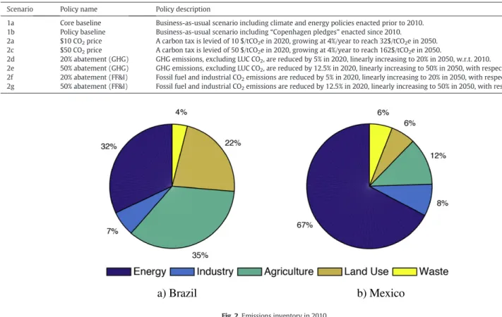
These starting positions result in two very different initial break-downs of GHG emissions.Fig. 2shows the reference emissions by sector for both countries. As shown, the share of energy related emissions is much higher in Mexico than in Brazil (67% vs. 32%), but land-use emis-sions are lower in Mexico than in Brazil (6% vs. 22%). Industrial sectors contribute with similar shares of emissions in both countries (8% and 7%, respectively).
In our Scenario 1a (Core Baseline), without policies to price carbon, electricity mixes reflect the economics of different technologies and their capacity to provide baseload, intermediate and peak power during the year, as well as local resources availability and proximity to energy markets. Our Scenario 1a (Core Baseline) results for primary energy are shown inFig. 3. EPPA estimates a total primary energy supply of 10.1 EJ in Brazil and 6.7 EJ in Mexico for 2010 (IEA data in 2010 for Brazil is 10.3 EJ and 7.4 EJ for Mexico (IEA, 2014a,e)).7
Table 2
LAMP/CLIMACAP scenario description.
Scenario Policy name Policy description
1a Core baseline Business-as-usual scenario including climate and energy policies enacted prior to 2010. 1b Policy baseline Business-as-usual scenario including“Copenhagen pledges” enacted since 2010.
2a $10 CO2price A carbon tax is levied of 10 $/tCO2e in 2020, growing at 4%/year to reach 32$/tCO2e in 2050. 2c $50 CO2price A carbon tax is levied of 50 $/tCO2e in 2020, growing at 4%/year to reach 162$/tCO2e in 2050.
2d 20% abatement (GHG) GHG emissions, excluding LUC CO2, are reduced by 5% in 2020, linearly increasing to 20% in 2050, w.r.t. 2010.
2e 50% abatement (GHG) GHG emissions, excluding LUC CO2, are reduced by 12.5% in 2020, linearly increasing to 50% in 2050, with respect to 2010. 2f 20% abatement (FF&I) Fossil fuel and industrial CO2emissions are reduced by 5% in 2020, linearly increasing to 20% in 2050, with respect to 2010. 2g 50% abatement (FF&I) Fossil fuel and industrial CO2emissions are reduced by 12.5% in 2020, linearly increasing to 50% in 2050, with respect to 2010.
5
For modeling purposes, we follow the CLIMACAP/LAMP Scenario protocol where the pledges were summarized in aggregate emission reductions for different regions in Sce-nario 1b (Policy baseline). The detailed Copenhagen pledges (UN, 2009) for each country can be found athttp://unfccc.int/meetings/copenhagen_dec_2009/items/5262.php.
6
A comparison of base year data and baseline trajectories are presented in this Special Issue, where the EPPA model outputs are benchmarked against IEA, UN and other data for the base year and for the projections from other models (van Ruijven et al., 2015).
a) Brazil
b) Mexico
Fig. 2. Emissions inventory in 2010.
7
The difference stems from an underestimation of biomass and geothermal energy, which are not disaggregated in the GTAP database.
In Brazil's 2010 primary energy mix, EPPA estimates a substantial contribution from hydro energy—1.6 EJ, or about 13%—and additional contributions from natural gas, coal and nuclear in shares of 9%, 5% and 1%, respectively. Our modeling results for 2010 agree with the IEA data (IEA, 2014a).8EPPA also estimates that Brazil relies heavily on oil and biomass for energy uses, with oil at 5 EJ and biomass at 2.5 EJ,9or 40% and 31% of total primary energy, respectively.
Since development of hydropower is limited by total resource availability, other energy sources start growing at a faster pace in the future projections of energy use. We calibrate EPPA to consider maximum total hydro resource potential for all basins in Brazil based on the National Energy Plan 2030 resource assessment (EPE, 2007). In the Amazon and Tocantins/Araguaia regions, we only consider hydro resource that could be developed without significant environmental impacts. Our results show that by 2050 Brazil will significantly increase use of natural gas, oil and biomass, with the renewable hydro and biomass covering 31% of energy needs. CLIMACAP/LAMP models project varying primary energy mixes—some models show higher use of coal (MESSAGE model) or biomass (POLES model) (van Ruijven et al., 2015).
In Mexico, fossil fuels supplied over 97% of energy in 2010, dominat-ing the primary energy mix. EPPA estimates oil use at 3.6 EJ, natural gas at 2.6 EJ and coal at 0.3 EJ. Hydro and nuclear account for 0.13 EJ and 0.6 EJ, or 2% and 1%, respectively. Again, the EPPA model numbers for 2010 are very close to the IEA statistics (IEA, 2014e). Considering that most of Mexico's economic hydropower potential has already been tapped in the baseline year, we project that Mexico will continue to rely almost entirely on fossil resources for its energy needs, with some increase in natural gas and oil use. In the absence of policy interventions, no other energy sources are expected to increase significantly. For Mexico, all CLIMACAP/LAMP models agree that fossil energy will domi-nate the mix in the Scenario 1a (Core Baseline) and only one model (POLES) projects solar resource deployment by 2050 (van Ruijven et al., 2015).
3.1. Electricity
Brazil starts with a cleaner electricity mix than Mexico. EPPA esti-mates that hydro energy supplies 79% of Brazil's electricity in 2010, followed by natural gas (9%), biofuels (5%), nuclear (3%), oil (2%) and wind and coal (1% each).10In contrast, fossil fuels comprise the majority
of Mexico's 2010 electricity mix, with natural gas (55%), coal (10%) and oil (9%), accounting for 74% of the mix. Other sources of electricity in-clude hydropower (17%), nuclear (8%) and biomass (1%).11
Fig. 4shows our projections for both countries' electricity mix up to 2050. Brazil continues to rely on hydropower, developing the potential of the North and Amazon basins; natural gas also increases, becoming a lower-cost resource due to reserves and discoveries of the pre-salt oil and gasfields. Mexico makes a rapid transition to natural gas technolo-gies, driven by lower-cost natural gas in North American markets and domestic policies allowing expansion of infrastructure for the extraction and distribution of natural gas.
3.2. Final energy use: industry, transportation and residential and commercial
In 2010, EPPA estimatesfinal energy use of 8.9 EJ for Brazil, and 4.9 EJ for Mexico. In 2050,final energy use grows in all sectors of both econo-mies, as shown inFig. 5, with industry and transportation consuming a majority of allfinal energy—77% in Brazil and 53% in Mexico. This result is based on the relative shares of the sectors in the base year, their ener-gy intensity, fuel andfleet mix, and improvements in energy efficiency. Energy efficiency improvements are driven by two major factors: price-and income-induced efficiency improvements and non-price induced technological changes, both are parameterized to historic responses as described inPaltsev et al. (2005),Webster et al. (2008)andChen et al. (2015).
3.3. Emission trends
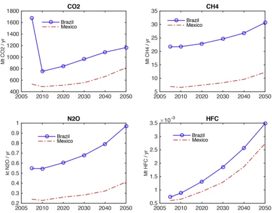
The resulting emission trends for Brazil and Mexico are shown in
Fig. 6. We show results for the trends projected by EPPA for 2050. It should be noted that deforestation control programs were put in place that caused Brazil's land-use emissions to decrease by 80% between 2005 and 2010. We impose a policy constraint on land-use emissions to reflect these regulations. Both countries' emission trajectories ended at almost the same level for CO2; however, compared to
Mexico, Brazil emits 3.5 times the amount of methane and twice the amount of nitrous oxide. The difference in non-CO2emissions can be
ex-plained by the greater amount of agriculture and cattle-raising econom-ic activities in Brazil.
Fig. 7shows the contribution of CO2emissions from combustion
pro-cesses and land-use change (to 2050)—an important distinction for mit-igation strategies. We assume that Brazil's successful deforestation control programs continue throughout the modeling period. Although
a) Brazil
b) Mexico
Fig. 3. Primary energy (Scenario 1a (Core Baseline)).
8
EPPA estimates 0.9 EJ (1 EJ real data) of natural gas, 0.5 EJ (0.6 EJ real data) and 0.1 EJ (0.2 EJ real data) of nuclear. In relative terms, the participation of the resources is the same in the EPPA model than in real data.
9 It is worth noting that the IEA reporting for biomass includes waste use for energy pur-poses, while EPPA includes only biofuels.
10
IEA data for 2010 for Brazil shows 78% hydro, 7% natural gas, 6% biofuels, 3% oil, 2% coal, and 0.4% wind (IEA, 2014b).
11
IEA data for Mexico for 2010 shows 52% gas, 16% oil, 12% coal, 14% hydro, 2% nuclear, 2% geothermal and 1% biomass (IEA, 2014f).
Fig. 6. Emissions trends for CO2(fossil and land use), methane, nitrous dioxide and F-gases (Scenario 1a (Core Baseline)).
a) Brazil
b) Mexico
Fig. 5. Final energy use by sector Scenario 1a (Core Baseline)).
a) Brazil
b) Mexico
significant levels of deforestation control enforcement are still needed to avoid the high levels of deforestation previously experienced in Brazil,12as 60% of its total area is still under natural vegetation we be-lieve a low and constant level of deforestation is a reasonable conserva-tive assumption.
4. Policy scenarios
Following the CLIMACAP/LAMP scenario protocol, we modeled seven policies: 1) Scenario 1b (Policy baseline): the Copenhagen climate mitigation pledges; 2) Scenario 2a ($10 CO2price): a carbon tax of $10/
tCO2e, starting in 2020 and increasing by 4% each year; 3) Scenario 2c
($50 CO2price): a carbon tax of $50/tCO2e, starting in 2020 and
increas-ing by 4% each year; 4) Scenario 2d (20% abatement (GHG)): a total emissions cap, reducing CO2e from 2010 levels 5% by 2020, 10% by
2030, 15% by 2040 and 20% from 2050 onwards; 5) Scenario 2e (50% abatement (GHG)): a stringent total emissions cap, reducing CO2e from
2010 levels 12.5% by 2020, 25% by 2030, 37.5% by 2040, and 50% from 2050 onwards; 6) Scenario 2f (20% abatement (FF&I)): a cap on CO2
emissions only, following the same reductions of Scenario 2d; and 7) Scenario 2 g (50% abatement (FF&I)): a cap on CO2emissions only,
fol-lowing the same reductions of Scenario 2e (SeeTable 2).13
We consider the Copenhagen pledges—voluntary commitments to reduce emissions by 2020—from both Brazil and Mexico. Brazil commit-ted to reductions of 36–39% from its business-as-usual (BAU) projection of 3236 Mt CO2e (MCTI, 2013), aiming for 1977–2068 Mt CO2e (a
reduction of 1168–1259 Mt CO2e) by 2020 (MCTI, 2013).14By 2010,
Brazil's emissions were already down to 1246 Mt CO2e—well below
the target (MCTI, 2013). If land-use emissions are kept under control, then even with very rapid growth in fossil and industrial emissions, Brazil will be well below the official Copenhagen target for its total emissions. Our estimate for Brazil's new business-as-usual (including reductions from 2005 to 2010) is around 1400 Mt CO2e in 2020—still
well below the Copenhagen target. We still require the industry to re-duce its emissions according to Brazil's sectoral specifications in the Co-penhagen pledges—a small requirement relative to Brazil's total emissions. Brazil has no further announcements of policy targets be-yond 2020; therefore, after 2020 we allow Brazil emissions to grow ac-cording to the Scenario 1b (Policy baseline).
Mexico has pledged to reduce CO2e emissions from its
business-as-usual scenario projection of 882 Mt CO2e (SEMARNAT, 2012) to about
620 Mt CO2e—about 30%. In the EPPA model, Mexico's 2005 emissions
correspond to the official data of about 700 Mt CO2e. However, unlike
the official business-as-usual estimates, we project a switch from coal and fuel oil to natural gas generation—an assumption supported by ac-tual changes in Mexico's energy sector, driven by imports of relatively cheap natural gas from the USA (IEA, 2013; Paltsev et al., 2011). As a re-sult, our business-as-usual projections place Mexico's 2020 emissions lower than the official projections—at about the same level as 2005 emissions. Therefore, in our projections Mexico starts out closer to its Copenhagen target than in the official estimate.
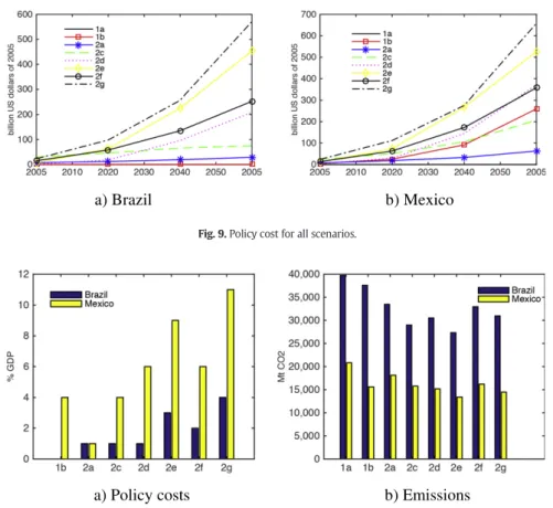
Fig. 8shows total emission trajectories in CO2e for each scenario,
andFig. 9shows the associated policy cost (measured as GDP loss in 2005 US dollars15). To facilitate policy comparison, inFig. 10we show total cumulative emissions and cost for each scenario. From the total
a) Fossil and Industry
b) Land Use
Fig. 7. CO2emissions Scenario 1a (Core Baseline)).
12Policies to reduce deforestation even further are not designed in Brazil yet and despite some discussion about“zero deforestation” in the country, there is no agreement about such target or its political feasibility.
13
Scenarios 2f and 2g were specified to provide a comparison with energy system only models.
14
The official business-as-usual projections do not consider emission reductions that oc-curred between 2005 and 2010.
15 We report all monetary results in 2005 US dollars, unless specified otherwise.
a) Brazil
b) Mexico
emissions trajectories, we see that both countries' Copenhagen pledges require very different mitigation efforts. In our Scenario 1a (Core Base-line), Brazil will require almost no additional mitigation, as the emis-sions reduction from deforestation control has already occurred.16For Mexico, our modeling results suggest that current policies implemented are aligned to reach the Copenhagen pledges by 2020, and the policy cost could be in the order of 4 billion US dollars in that year.
Our analysis shows the differences between two distinctive policy instruments: carbon taxes and emissions quantity constraints. Key con-siderations for new policies are cost totals and timing, and the total cost and timing of each policy can change depending on the prices and con-straints imposed each decade, as explained inTable 2.17
Brazil and Mexico both see similar results in Scenario 2a ($10 CO2
price), which resulted in slower reduction atfirst, but ultimately a great-er emissions reduction in the end. Brazil and Mexico also show similar results in Scenario 2c ($50 CO2price) and Scenario 2d (20% abatement
(GHG)). Total cumulative emissions are comparable, as are the total pol-icy costs (as shown inFig. 10b). However, a key difference between Scenarios 2c and 2d is that these costs occur at different points in time (seeFig. 9a and b). For Brazil, Scenario 2c has a higher total economic cost than Scenario 2d in 2020, but by 2050 their relative costs are re-versed. Scenario 2c requires more abatement early on, but once new technologies are in place as a result of the tax, lower costs are incurred at the end of the period. Scenario 2d has a lower cost early on, but the
relatively relaxed cap delays technology deployment, increasing later costs and ultimately requiring additional abatement from all sectors. We observe these same dynamics in Mexico, although to a much lesser extent.
All scenarios imply increased GDP losses from 2020 to 2050, ranging from 1–11% for Mexico and 0–4% for Brazil (Fig. 10a). For both countries, policy costs are the highest in Scenario 2e (50% abatement (GHG)) and Scenario 2 g (50% abatement (FF&I)).
It is worth comparing the carbon prices resulting from emissions caps. For example, in Scenario 2e (50% abatement (GHG)), carbon prices for 2020, 2030 and 2050 in Brazil are $9/tCO2e, $74/tCO2e, and $386/
tCO2e, respectively. The corresponding prices in Mexico are $17/tCO2e,
$101/tCO2e, and $437/tCO2e. In Scenario 2c ($50 CO2price), both
coun-tries have a tax that is equivalent to $50/tCO2e in 2020 and reaching
$162/tCO2e in 2050. For the cap Scenarios 2d, 2e, 2f and 2 g, lower
car-bon prices in the initial periods lead to higher prices in the later periods in comparison to the tax Scenarios 2a and 2c.
Our results suggest that even Scenario 2a ($10/tCO2e tax), the
lowest-cost policy, could have a significant impact on total emissions trajectories. Compared to the Scenario 1a (Core Baseline), Scenario 2a ($10/tCO2e tax) reduces total cumulative emissions by 25% in Brazil
and 28% in Mexico. In contrast, Scenario 2e (CO2e cap, 50% by 2050)
re-duces total cumulative emissions the most—by 50% in Brazil and 60% in Mexico—but also costs 10 and 7 times more for Brazil and Mexico, re-spectively. The cumulative costs of Scenario 2c ($50/tCO2e tax) are
about 4 times higher than Scenario 2a ($10/tCO2e tax).18
In the following sections we describe some of the changes occurring in each scenario in terms of energy use, technology deployment in rele-vant sectors and land-use changes.
16
Brazil reduced deforestation from an average of 2.6 million ha in the period 2000 to 2005 to less than 0.7 million ha after 2010. This policy was incorporated in the Brazilian Copenhagen pledges in 2009 and confirmed by Law 12.187, The National Plan on Climate Policy, enacted in December 2009 (WRI, 2010). Policies to reduce deforestation even fur-ther are not designed in Brazil yet and despite some discussion about“zero deforestation” in the country, there is no agreement about such target or its political feasibility.
17
In this exercise we have not accounted for cost inter-temporal discounting (consider-ing different discount rate factors), which is someth(consider-ing that policy makers could take into account.
18
Policy costs vary widely among models in the CLIMACAP/LAMP exercise; for a discus-sion of macroeconomic impacts seeSummerton et al. (2015).
a) Policy costs
b) Emissions
Fig. 10. Cumulative policy costs and emissions for all scenarios (2010–2050).
a) Brazil
b) Mexico
4.1. Energy consumption and energy efficiency
Brazil and Mexico have several options for emission reductions: to use existing lower-carbon technology, to deploy new low-carbon tech-nologies into their production processes andfinal energy use, and in-creases in energy efficiency. In addition to exogenously specified energy efficiency improvements, EPPA models the price-induced and income-induced energy efficiency improvements that lead to a substan-tial demand response resulting from policy implementation. Demand response is parameterized based on historic responses to energy price
increases (Webster et al., 2008). The resulting energy consumption is af-fected both by demand and supply responses.
For example, in Scenario 2a ($10/tCO2e tax),final energy use in 2050
decreases by 9% in both Mexico and Brazil, compared to the Scenario 1a (Core Baseline). In Scenario 2c ($50/tCO2e tax), the corresponding
num-bers are 27% for Mexico and 22% for Brazil. Comparing these responses from the EPPA model to the other models in the CLIMACAP/LAMP exer-cise, one can notice that there are two types of the model responses in this respect: those that calculate energy efficiency improvements and demand responses, and those with relatively inelastic demand. For
a) Brazil
b) Mexico
Fig. 11. Mitigation in the electricity sector.
example, in Scenario 2c ($50/tCO2e tax), the more responsive IMAGE,
Phoenix, GCAM and LEAP-UNAM models show a 15%–35% reduction infinal energy use for Mexico and Brazil, while the relatively inelastic TIAM-ECN, POLES, and MESSAGE models show a reduction of 4–8% for Brazil and 5–14% for Mexico (Lucena et al., 2015; Veysey et al., 2015). Driven by energy efficiency improvements and other factors mentioned above, energy intensity of GDP also decreases in response to these pol-icy changes. EPPA results show that by 2050, energy intensity decreases from baseline in both Scenario 2a ($10/tCO2e tax), 7% in Mexico, and 8%
in Brazil, and Scenario 2c ($50/tCO2e tax), 22% in Mexico and 20% in
Brazil.
4.2. Low-carbon electricity technologies deployment
As shown inFig. 11, in the Scenario 2d (20% abatement (GHG)) and Scenario 2e (50% abatement (GHG)), Brazil continues to use its hydropow-er, adding natural gas, biomass and more wind. Since Brazil has a clean electricity mix to start with, it is harder to reduce carbon emissions
Fig. 14. Mitigation in the Mexican industrial sector. Fig. 13. Energy use in the Brazilian industrial sector.
from electricity sector in Brazil, but there is substantial mitigation poten-tial from agriculture, and existing low-carbon technologies can be brought into the energy mix. Due to high capital requirements and sunk costs of old projects, Brazil's hydropower is not as responsive to carbon pricing as other generation technologies. When economy-wide emission constraint is imposed in Brazil, wefind that the most economic option is to mitigate in the agricultural sector. In contrast, Mexico's most economic option is to deploy new advanced technologies, such as natural gas and coal with CCS.
The models in the CLIMACAP/LAMP exercise present a large range of the results regarding technology deployment. However, all models agree that in a comparison of Scenario 2e (50% abatement (GHG)) to Scenario 1a (Core Baseline), Brazil's fossil energy use decreases, and Mexico will deploy natural gas with CCS. Most models agree that Brazil will substantially expand biomass, wind and solar use, and that Mexico will deploy substantial biomass generation or expand use of other renewables (Lucena et al., 2015; Veysey et al., 2015).
While we focus in the 2050 horizon in this paper, in the CLIMACAP/ LAMP scenarios we estimated results up to 2100. We found other tech-nologies playing a significant role later in the period, as population and
economic trends increasingly require more energy despite the emis-sions cap. The electric power sector boosts its zero-carbon technologies in the second half of the century. Wind and solar technologies increase penetration in the second half of the century in all scenarios. There are two sets of reasons for this relatively late penetration compared to other CLIMACAP/LAMP models (seevan der Zwaan et al. (2016a)). First, our model considers the costs of replacing existing infrastructure in the different regions (some models do not fully internalize the costs of vintaged capital), as well as institutional costs that slow the penetra-tion of new technologies in the model (as a funcpenetra-tion of installed capacity in the previous period). Second, to account for reliability constraints, the intermittent nature of renewables in our model is taken care of by im-posing a requirement of full back-up capacity for large-scale penetration of renewables, either with natural gas turbines or bioelectricity plants.
Thus, in Mexico wefirst see a transition towards natural gas technol-ogies, which are competitive both because of low natural gas prices in the region and because they are dispatchable technologies. The model then progresses to the deployment of wind and solar generation as those technologies become competitive.19
The deployment of low-carbon electricity technologies is of great in-terest for policy makers; however, several uncertainties arise regarding future technology costs. For example, innovation and deployment of re-newable energy technologies around the world could rapidly decrease the costs of solar and wind energy. The International Energy Agency es-timates a learning rate for these technologies in the order of 5% for bio-mass, geothermal and onshore wind, 18% for solar PV and 10% for CSP (IEA, 2014c). The US Energy Information Administration studies also project future cost reductions both in renewables and in CCS technolo-gies. EPPA's electricity cost assumptions are based onEIA (2014). Technology costs are reduced over time for all technologies based on
19 More detailed studies are needed to better incorporate the operational constraints of power systems with large-scale penetration of renewables, and the need forflexibility op-tions such as storage technologies and transmission and distribution networks that will be needed to increase the current systemflexibility (Octaviano et al., 2015).
Fig. 16. Oil net exports (Scenario 1a (Core Baseline) and Scenario 2g (50% abatement (FF&I))). Fig. 15. Energy use in the transportation sector.
the EIA projections.EIA (2014)reports that the levelized cost of solar electricity in 2040 is still more than 40% higher than natural gas with CCS; thus, the EPPA model installs more natural gas than solar in Mexico. Similar results regarding the economics of current solar tech-nologies are found byFrank (2014). Wind energy has a competitive levelized cost of electricity, but once we account for intermittency costs, wind also penetrates slowly. Given the uncertainties regarding technology costs and potential deployment under carbon policy, we be-lieve that there could be value in portfolio diversification. EPPA does not deploy renewables at scale during thefirst decades of climate policy im-plementation (2020–2050), but the large-scale deployment of renew-ables needed for deep decarbonization (2050–2100) could justify policies for early technology deployment to prepare the energy transi-tion, such as those currently under consideration by the Mexican gov-ernment (SENER, 2013).
Storing CO2with CCS technologies at scale imposes a technological
challenge (Herzog, 2001) and the storage capacity and rate of deploy-ment must be taken into consideration, including the developdeploy-ment of adequate regulatory frameworks and incentives to avoid potential leak-age issues (i.e., high penalties and standards for site construction). The largest cumulative amount of stored carbon from CCS technology is about 4 Gt CO2by 2050 in Scenario 2e (50% abatement (GHG)). The
Mex-ican government has started the development of a National Strategy for CO2Carbon Capture and Storage (SENER, 2014) and the mapping of
po-tential sites and storage capacity (SENER/CFE, 2014) with a preliminary estimate of the total carbon storage theoretical potential of 111 Gt CO2.
4.3. Land-use changes
Careful analysis of policy-driven land-use changes is of the utmost importance in the region. While agriculture contributed with 5% and 3% of total GDP of Brazil and Mexico in 2010, the population working on this sector is 17% in Brazil and 13% in Mexico (WB, 2014). Much of the economically vulnerable population, including poor households and indigenous communities, depend on this activity. Thus, the conse-quences of policy on farmers and communities in Brazil and Mexico are of special concern. In addition to providing important ecosystem services (e.g. carbon sequestration), the forests and other ecosystems in Brazil and Mexico provide critical biodiversity—both Brazil and Mexico are among the 17 megadiverse countries of the world (Groombridge, 1994). In the past, economic growth has driven an ex-pansion of agriculture and pasture at the expense of forests and other ecosystems. EPPA provides a high-level analysis of economic incentives that will drive land conversion under different scenarios.Fig. 12shows EPPA model estimates for land uses in Brazil and Mexico as a result of expected land conversion in the Scenario 1a (Core Baseline).
For our baseline scenario, we consider the policies that Brazil and Mexico have already implemented to reduce deforestation. For Brazil, without additional policy efforts, total land-use emissions are set to
maintain 2010 levels, but total cropland still expands from 8 to 22% due to increasing food demand and biofuels production. This expansion comes from conversion of other arable land (6%) and forests (8%). Pas-ture also expands from 17% to 19%, at the expense of forests. Mexico has implemented policies to slow deforestation rates, but they are still high. Without further policy efforts, Mexico's cropland expansion will come at the expense of forests and other arable land. Forest cover in Mexico is projected to decrease from 38% of the total land area in 2010 to 28% by 2050.20
4.4. Industry and transport
Brazil's industrial use of electricity, liquids, natural gas and coal in-creases over time in the Scenario 1a (Core Baseline). In all policy scenar-ios their use is lower than in the Scenario 1a (Core Baseline) (Fig. 13). In Mexico, industrial use of electricity, natural gas and liquids is growing over time in the Scenario 1a, while coal use is slightly reduced after 2020 due to natural gas substitution (Fig. 14).
In the policy scenarios, coal, electricity, and natural gas use de-creases, while liquid use increases. The reason for these small increases in liquid use in the policy scenarios is the drop in the domestic price of oil sub-products that enter as feedstock inputs to production in the pro-cesses of chemical and petrochemical industries.
In both countries, the transportation sector increases energy use over time in the Scenario 1a (Core Baseline). As shown inFig. 15, the more stringent emission reduction scenarios lead to substantial de-creases in energy use. Scenario 2e (50% abatement (GHG)) reduces transportation energy use by 30% for Brazil and 34% for Mexico. These percentages increase to almost 50% in Scenario 2 g (50% abatement (FF&I)). For Brazil, the two tax scenarios increase bioenergy production, while the two cap scenarios decrease it; for Mexico, biofuel production increases in all scenarios, but remains relatively small given low flex-fuelfleet in the country.
These results underscore the relevance of the transportation sector in mitigation, and the need for alternatives to efficiently reduce its ener-gy use (e.g., morefleet flexibility, public transportation or cleaner tech-nologies such as public and private modes of electric transportation). Further research in this area is recommended to evaluate the cost-effectiveness of different transportation modes in Brazil and Mexico with the goal of reducing GHG emissions—this may aid policy makers in focusing policy efforts.
4.5. Energy trade
In this section, we briefly provide some context on energy trade in both countries and explore some alternatives for oil production devel-opment in Brazil and natural gas imports in Mexico. Both Mexico and
20
For a comparison to land use results from other models seeCalvin et al. (2016-in this issue). Fig. 18. Brazil's net imports.
Brazil are currently experiencing profound changes in their oil and gas sectors, although the two differ in the state of development of their petroleum industries. Mexico has been exporting oil since the 1970's; its main oilfields appear to have reached maturity, and some fields show a substantial decay in production. This situation has resulted in a major energy reform to canalize private investment in order to revitalize oil production. Brazil is not quite self-sufficient in terms of oil (BP, 2014b; IEA, 2013), though analysts and policy makers in Brazil expect future oil exports, following developments in deep water sites (BP, 2014a; IEA, 2014d, 2013).
Uncertainties surround the future development of the oil industry in both countries, but we project that both will be able to revitalize their oil industries if the resources are developed adequately and with needed investment. To account for potential technological challenges, for Brazil, we consider two variations of the Scenario 1a (Core Baseline) with different rates of resource development. As presented inFig. 16, our modeling results suggest that Mexico could increase its exports above 2 million barrels per day (Mbd) from 2020 to 2050, and Brazil could export between 0.9 and 1.3 Mbd for the same period. In both cases, our estimates of potential production levels for 2020 are in corre-spondence with the estimates by IEA (IEA, 2014d). Without climate pol-icy, oil exports peak in the 2030's for both countries. If new oilfields in Brazil are developed at a slower pace (Core Baseline—slow oil develop-ment), then oil exports start declining as domestic production is used to meet fast-growing domestic oil demand; and by 2040 Brazil becomes a net importer of oil once again.
Oil exports are reduced when climate policy is implemented because explicit or implicit carbon price makes oil more expensive for con-sumers, which results in reduced demand for oil. In addition, there is some economic contraction that leads to a reduction in overall demand as well. For example, Scenario 2 g (50% abatement (FF&I)) results in re-duced oil exports of 13% for Mexico and 47% for Brazil (relative to Core
Baseline - fast oil development). Under Scenario 2 g (50% abatement (FF&I)), oil exports peak in 2030 for Mexico and in 2020 for Brazil.
In addition to oil export dynamics, wefind that Brazil increases bio-fuel exports in all scenarios, particularly under the tax scenarios; how-ever, even in Scenario 2 g (50% abatement (FF&I)) Brazil's biofuel exports are only about 0.2 EJ, indicating that biofuels are not likely to play a major role in Brazil's energy exports (Fig. 17). In the Scenario 1a (Core Baseline), both countries are net importers of refined oil prod-ucts and coal (except for Brazil in 2030, which is affected by our as-sumption of fast oil development), as shown inFigs. 18 and 19. For all policy scenarios, Brazil reduces its coal imports. Brazil also increases its imports of refined oil products, particularly in 2050, when domestic demand is substantially higher than national oil production. For Mexico, coal imports are generally low (below 0.01 EJ in most scenarios), but they increase in some scenarios as a result of an increased coal use in the power sector (with CCS technologies).
Natural gas is of strategic importance for Mexico—it is expected to meet most of the power sector energy demand, and it also plays a major role for industrial use (seeSections 4.2 and 4.4). Thus, we detail our modeling assumptions for natural gas and provide the reference sta-tistics regarding natural gas trade in Mexico as a benchmark for our modeling results. In 2010, domestic demand for natural gas in Mexico was 6341 million cubic feet per day (mmcfd) and production was 5004 mmcfdm, resulting in net imports21of 1337 (SENER, 2013). De-mand and production estimates in EPPA are 10% higher than historical figures in 2010, with the same level of imports. The Mexican govern-ment estimates that, by 2027, Mexico will reach production of 6848 mmcfd (the EPPA estimate for 2025 is 6721). By 2050, EPPA estimates Mexico's domestic production of natural gas to be
a) Coal
b) Refined Oil Products
Fig. 19. Mexico's net imports.
21
Total imports were 1458 mmcfd, exports 83 mmcfd, and a statistical difference of 38 mmcfd.
12,552 mmcfd, requiring additional imports of 2117 mmcfd to satisfy demand in that year. In order to keep imports below this level (between 14 and 20% of total demand) domestic production in the country needs to maintain a fast-paced growth to match demand (Fig. 20). If invest-ments in domestic natural gas resources and infrastructure are not ad-equate, Mexico could meet its natural gas demand with imports rather than domestic production.22
Climate policy in Mexico reduces both domestic production and con-sumption of natural gas. As the policy is implemented globally, natural gas price in the USA (a major exporter of natural gas to Mexico) is re-duced, which makes it un-economic to develop more costly resources both in the USA and Mexico. Our modeling results show that in Scenario 2 g (50% abatement (FF&I)), Mexico's natural gas imports decrease by 48% from the Scenario 1a (Core Baseline) by 2050.
It is worth mentioning that without investments in oil and gas, Mexico and Brazil could substantially increase their imports of both re-sources. Due to the previously discussed technological and institutional uncertainties, the risks involved in the development of these resources should be considered when crafting climate policy, along with the po-tential co-benefits (e.g. reduced fuel imports) and interactions with other policies addressing energy security matters. Brazil can rely in its hydropower resources for electricity generation; Mexico, on the other hand, will have to heavily rely on imports of natural gas if local re-sources remain difficult to tap. In addition, if energy investment into oil exploration and exploitation is not timely, or if the results are unsuc-cessful for technical reasons, oil imports will be necessary to satisfy growing demand for transportation and industrial uses.
5. Conclusions
We have evaluated climate policy options and their implications for the two largest Latin American economies: Brazil and Mexico. Wefind that there are substantial differences between the impacts on economy and energy systems in these two countries. The dominant low-carbon technologies are hydropower, wind and biomass for Brazil, and carbon capture and storage, hydropower and nuclear in Mexico. Meeting sub-stantial emission reduction targets requires large-scale changes in their energy systems—in the most stringent policy scenario (a 50% re-duction of all GHGs by 2050 relative to 2010 levels), both countries fully decarbonize electricity. The cost of reaching ambitious reduction targets also differs—from 2020 to 2050, GDP losses range from 4 to 11% for Mexico and 0–4% for Brazil.
GHG emission reduction requires substantial changes in energy, ag-riculture and land use practices. An analysis that encompasses energy and other economic sectors—such as the one we present using the MIT EPPA model—is valuable to investigate the full mitigation potential of the Latin American countries. For instance, when climate policy covers only fossil fuel and industrial emissions, costs are 33% higher in Brazil and 22% higher in Mexico compared to a policy design that covers all economic sectors. This result confirms that economy-wide emission trading mechanisms could substantially reduce mitigation costs. We find a large mitigation potential could be realized in these two countries for the period 2010–2050, in the order of 12.4 Gt CO2e cumulative
emis-sions reduction in Brazil and 7.4 Gt CO2e cumulative emissions
reduc-tion in Mexico.
Due to the global nature of GHG impacts, a successful agreement to limit climate change requires global participation. Mitigation by even the largest emitters alone would not solve the problem (Paltsev et al., 2012)—actions are needed from all emitters. Brazil and Mexico have taken what they consider to be nationally appropriate mitigation actions—Brazil has already decreased emissions below its Copenhagen
pledges, and Mexico has implemented policies that are consistent with its 30% emissions reduction goal. Going forward, extensive discus-sions remain regarding their future contributions to mitigation. So far, international climate negotiations face the challenge offinding a “fair” scheme for each individual country's contributions to global GHG emis-sion reduction. There are numerous proposals for burden sharing (IPCC, 2014) that calculate equal percentages, equal marginal cost or same car-bon price among the countries. Studies have shown that a global carcar-bon tax or cap-and-trade system is an efficient way to reduce emissions; however, recent approaches (discussed at the UN conferences in Copen-hagen (UN, 2009) and Cancun (UN, 2010)) focus on national plans that differ from country to country. The results of our study justify the Co-penhagen–Cancun approach.
For Brazil and Mexico, we found that because of differences in ener-gy and land use emissions sources, same carbon prices and emission caps lead to very different policy costs—specifically, cumulative costs in Mexico are about twice as high as those in Brazil. Another difference is that the largest share of Mexico's GHG emissions comes from energy, while in Brazil agricultural activities are responsible for the largest share. Therefore, a policy that targets only energy emissions would not affect the largest sources of emissions in Brazil. Energy efficiency plays an important role in mitigation scenarios for both countries, and energy and electricity uses are reduced in all policy scenarios relative to a no-policy scenario. In all climate policy scenarios, Brazil continues to rely on hydropower with some additional electricity from wind, bio-mass and natural gas, particularly in Scenario 2e (50% abatement (GHG)) and Scenario 2g (50% abatement (FF&I)), while Mexico employs CCS substantially on fossil-based generation. Land-use emissions policies are important to consider in both countries; especially in Brazil, land-use policies change the total economic costs of different energy policies, as discussed byGurgel and Paltsev (2014). In this study, we assumed that current policies to control deforestation would be kept in place. We underscore the importance of these deforestation policies (which should not be confused with a no-policy world). Without strict control, high rates of deforestation could occur in Brazil and Mexico, with detri-mental impacts on climate change and regional ecosystems. Brazil's de-forestation emissions reduction policy should be maintained; Mexico should use Brazil's example to reduce its land use emissions.
Our study confirms that climate policies proposed in Copenhagen and Cancun by Brazil and Mexico are solid steps in the right direction, and that further mitigation actions should be considered in light of dif-ferentiated costs across countries, their starting position, and differing national capacities. Though many challenges lie ahead in the process of further GHG mitigation in Mexico and Brazil, continuing to develop strategies tailored tofit each country's energy and land use composition is a plan that should be maintained. We nevertheless underscore the need for all national strategies to add up to the UNFCCC goals of climate stabilization to prevent dangerous anthropogenic interference with the Earth's climate. Our study illustrates the difficulties underlining the dis-cussions of burden sharing with developing countries, given different economic structures and emissions profiles. Even among countries that share similar levels of development, and that have agreed to start mitigation action, moving towards deep mitigation implies different costs and benefits that need to be considered through national lenses. Acknowledgments
The authors gratefully acknowledge thefinancial support for this work provided by the Mario Molina Center, the National Council for Sci-ence and Technology of Mexico (CONACYT) and the National Council for Research of Brazil (CNPq). Thanks are due to Jamie Bartholomay for her help with the manuscript preparation and three anonymous reviewers for their useful suggestions. The MIT Emissions Prediction and Policy Analysis (EPPA) model is supported by a consortium of government, in-dustry, and foundations sponsors of the MIT Joint Program on the Science and Policy of Global Change, including the U.S. Department of
22Currently, Mexico has been experiencing acute infrastructure bottlenecks that have increased the imports of natural gas. In 2010, about 47% of the imports were identified by the Ministry of Energy as“logistic-imports” meaning those required due to lack of pipe-lines and other infrastructure to use local resources (SENER (2013)).
views of the European Union or the U.S. government. References
BP, 2014a. BP Energy Outlook 2035. BP (http://www.bp.com/en/global/corporate/about-bp/ energy-economics/energy-outlook/country-and-regional-insights/brazil-insights.html). BP, 2014b. Statistical Review of World Energy 2014. BP (http://www.bp.com/en/global/
corporate/about-bp/energy-economics/statistical-review-of-world-energy.html). Calvin, K., Beach, R., Gurgel, A., Labriet, M., Rodriguez, A.M.L., 2016.Agriculture, forestry, and
other land-use emissions in Latin America. Energy Econ. 56, 615–624 (in this issue).
Chen, H., Paltsev, S., Reilly, J., Morris, J., Babiker, M., 2015.The MIT EPPA6 Model: Econom-ic Growth, Energy Use, and Food Consumption. Report: No. 278. MIT Joint Program on the Science and Policy of Global Change, Cambridge, MA.
Da Motta, R.S., Hargrave, J., Luedemann, G., Gutierrez, M.B.S., 2011.Climate Change in Brazil Economic, Social and Regulatory Aspects. Institute for Applied Economic Research.
Dimaranan, B., McDougall, R., 2002.Global Trade, Assistance, and Production: The GTAP 5. Center for Global Trade Analysis, Purdue University, West Lafayette, Indiana.
EIA, 2014.Levelized Cost and Levelized Avoided Cost of New Generation Resources in the Annual Energy Outlook 2014. US Energy Information Administration.
EPE, 2007.Plano Nacional de Energia 2030. Chapter 3. Geracao Hidrelectrica. Empresa de Pesquisa Energetica.
EPE, 2013. Plano Decenal de Expansa˜o de Energia 2022. Empresa de Pesquisa Energe'tica (http://www.epe.gov.br).
Frank, C.R., 2014.The Net Benefit of Low and No-Carbon Electricity Technologies. The Brookings Institution.
Galindo, L.M., 2009.La economıa del cambio climatico en Mexico. SHCP/SEMARNAT.
Government of Brazil, 2008.National Plan on Climate Change Brazil (Executive Summary). Interministerial Committee on Climate Change (Vol. Decree No. 6263 of November 21, 2007).
Groombridge, B. e, 1994.Biodiversity Data Sourcebook. WCMC Biodiversity Series No 1. World Conservation Monitor Centre. The World Conservation Union, United Nations Environment Programme, World Wide Fund for Nature. World Conservation Press.
Gurgel, A.C., Paltsev, S., 2014.Costs of reducing GHG emissions in Brazil. Clim. Pol. 14 (2), 209–223.
Gurgel, A., Reilly, J., Paltsev, S., 2007.Potential land use implications of a global biofuels industry. J. Agric. Food Ind. Organ. 5 (2), 1–34.
Hertel, T., 1997.Global Trade Analysis: Modeling and Applications. Cambridge University Press, Cambridge, UK, Cambridge University.
Herzog, H., 2001.What future for carbon capture and sequestration? Environ. Sci. Technol. 35 (7), 148A–153A.
Hyman, R., Reilly, J., Babiker, M., Masin, A.V.D., Jacoby, H., 2003.Modeling non-CO2
green-house gas abatement. Environ. Model. Assess. 8 (3), 175–186.
IEA, 2013.World Energy Outlook 2013. International Energy Agency.
IEA, 2014a.Brazil: Balances for 2010. International Energy Agency.
IEA, 2014b.Brazil: Electricity and Heat for 2010. International Energy Agency.
IEA, 2014c.IEA World Energy Investment Outlook 2014: Annex A. Investment Tables. In-ternational Energy Agency.
IEA, 2014d.Mexico: Balances for 2010. International Energy Agency.
IEA, 2014e.Mexico: Electricity and Heat for 2010. International Energy Agency.
IEA, 2014f.Medium-Term Oil Market Report 2014. Market Analysis and Forecasts to 2019.
IPCC, 2014.Climate Change 2014: Mitigation of Climate Change. Cambridge University Press, Cambridge, United Kingdom and New York, NY, USA.
Lucena, A.F.P., Clarke, L., Schaeffer, R., Szklo, A., Rochedo, P.R.R., Daenzer, K., Gurgel, A., Kitous, A., Kober, T., 2016.Climate policy scenarios in Brazil: a multi-model compar-ison for energy. Energy Econ. 56, 564–574 (in this issue).
Margulis, S., Dubeux., C.B.S., 2011.The Economics of Climate Change in Brazil. Costs and Opportunities. FEAUSP.
McFarland, J.R., Reilly, J.M., Herzog, H.J., 2004.Representing energy technologies in top-down economic models using bottom-up information. Energy Econ. 26 (4), 685–707.
Octaviano, C., Ignacio, P., Reilly, J., 2015.The value of electricity storage: a hybrid modeling approach. MIT Joint Program on the Science and Policy of Global Change (Report).
Paltsev, S., Reilly, J., Jacoby, H., Eckhaus, R., McFarland, J., Saforim, M., Asadoorian, M., Babiker, M., 2005.The MIT Emission Prediction and Policy Analysis (EPPA) model: ver-sion 4. Report: No. 125. MIT Joint Program on the Science and Policy of Global Change, Cambridge, MA.
Paltsev, S., Jacoby, H., Reilly, J., Ejaz, Q.J., O'Sullivan, F., Morris, J., Rausch, S., Winchester, N., Kragha, O., 2011.The future of U.S. natural gas production, use, and trade. Energy Pol-icy 39 (9), 5309–5321.
Paltsev, S., Morris, J., Cai, Y., Karplus, V., Jacoby, H., 2012.The role of China in mitigating climate change. Energy Econ. 34 (S3), S444–S450.
SEMARNAT, 2012.México Quinta Comunicación Nacional ante la Convención Marco de las Naciones Unidas sobre el Cambio Climático. Secretarıa de Medio Ambiente y Recursos Naturales. Ministry of the Environment and Natural Resources of Mexico.
SEMARNAT, 2013.Inventario Nacional de Emisiones de Gases de Efecto Invernadero 1990– 2010 (National Inventory of Greenhouse Gas Emissions 1990–2010). Secretaría de Medio Ambiente y Recursos Naturales (Ministry of Environment and Natural Re-sources, Federal Government of Mexico).
SEMARNAT, 2014.Programa Especial de Cambio Clima'tico 2014–2018. (Special Program for Climate Change 2014–2018). Secretaría de Medio Ambiente y Recursos Naturales. (Ministry of the Environment and Natural Resources of Mexico).
SENER, 2013.Prospectiva de Gas Natural y Gas L.P. (Natural Gas and L.P. Gas Prospectives). Secretaría de Energía (Ministry of Energy, Federal Government of Mexico).
SENER, 2014. Estrategia Nacional de Captura. Uso y Almacenamiento de CO2. Retrieved May 1, 2014 (http://co2.energia.gob.mx/portal/default.aspx?id=2168).
SENER/CFE, 2014.Atlas de Almacenamiento Geológico de CO2en Mexico. Secretaría de
Energía (Ministry of Energy, Federal Government of Mexico) and Comision Federal de Electricidad (Federal Comission for Electricity).
Summerton, P., Pollitt, H., Chewpreecha, U., Ren, X., Wills, W., Octaviano, C., McFarland, J., Espinosa, Calderon, S., Fisher-Vanden, K., Rodriguez, A., 2016.The macroeconomic impact of climate mitigation action in Latin America: a model comparison. Energy Econ. 56, 625–636 (in this issue).
UN, 2009.Copenhagen Accord. United Nations Framework Convention on Climate Change.
UN, 2010. Cancun Agreements. United Nations Framework Convention on Climate Change (http://cancun.unfccc.int/).
UN, 2013. World Population Prospects: The 2012 Revision. Population Division, United Nations Department of Economic and Social Affairs (http://esa.un.org/unpd/wpp/ Excel-Data/population.htm).
van der Zwaan, B.C.C., Calvin, K., Clarke, L., (Guest Editors), 2016a.Climate Mitigation in Latin America: implications for energy and land use, Introduction to the Special Issue on thefindings of the CLIMACAP-LAMP project. Energy Econ. 56, 495–498.
van der Zwaan, B., Kober, T., Calderon, S., Modeller, G., Daenzer, K., Kitous, A., Labriet, M., Frossard Pereira de Lucena, A., Octaviano, C., di Sbroiavacca, N., 2016.Energy technol-ogy roll-out for climate change mitigation: a multi-model study for Latin America. Energy Econ. 56, 526–542 (in this issue).
van Ruijven, B., Calvin, K., Daenzer, K., Fisher-Vanden, K., Kitous, A., Kober, T., Paltsev, S., 2016.The starting points: base-year assumptions and baseline projections for Latin America. Energy Econ. 56, 499–512 (in this issue).
Veysey, J., Octaviano, C., Clarke, L., Martinez, S.H., Kitous, A., McFarland, J., van der Zwaan, B., 2016.Pathways to Mexico's climate change mitigation targets: a multi-model analysis. Energy Econ. 56, 587–599 (in this issue).
WB, 2014. World Development Indicators dataset. World Bank National Accounts Data, and OECD National Accounts Data Files. The World Bank (http://data.worldbank.org/). Webster, M., Paltsev, S., Reilly, J., 2008.Autonomous efficiency improvement or income
elasticity of energy demand: does it matter? Energy Econ. 30 (6), 2785–2798.