Carlos Pestana Barros & Nicolas Peypoch
A Comparative Analysis of Productivity Change in Italian and Portuguese Airports
WP 006/2007/DE _________________________________________________________
Luís M. S. Coelho, Rúben M. T. Peixinho, Siri Terjensen
Going concern opinions are not bad news:
Evidence from industry rivals
WP 16/2012/DE _________________________________________________________
De pa rtme nt o f Ec o no mic s
W
ORKINGP
APERSISSN Nº 0874-4548
Going concern opinions are not bad news:
Evidence from industry rivals
Luís Miguel Serra Coelho∗, #
School of Economics - University of the Algarve and CEFAGE
Rúben Miguel Torcato Peixinho#
School of Economics - University of the Algarve and CEFAGE
Siri Terjensen
Kelley School of Business - University of Indiana
ABSTRACT: This paper examines whether going concern audit opinions (GCO) affect the stock price performance of the announcing firms and their industry rivals. Our original evidence clearly suggests that such accounting event is asymmetrically perceived by the market depending on whether the firm is qualified by the auditor or not. In particular, firms receiving a GCO earn negative abnormal returns at the audit report’s disclosure date and over the following year whereas their industry rivals exhibit positive abnormal returns at the GCO date and in the subsequent one-month period. This is in contrast with the preevent abnormal returns, which, on average, are negative and significant for all firms operating within the industry. Overall, we highlight the relevance of audit opinions and mandatory accounting information for the timing of transactions in financial markets.
Keywords: Audit reports, going concern, competitive effect
Data Availability: The data used in this study are publicly available through sources identified in this study
∗ Contacting author: Luís Coelho, Assistant Professor of Finance, School of Economics -University of the Algarve,
Campus de Gambelas, Edifício 9, 8005-105 Faro – Portugal, Telephone: 00351 289 800915, Fax: 00351 289
800063, E-mail:[email protected]
#
Different versions of this paper have benefited from the comments, inter alia, of Richard Taffler, and participants at research seminars at University of Évora and Technical University of Lisbon. Luís and Rúben acknowledge
2
I. INTRODUCTION
The going-concern principle is one of the most basic in accounting assuming that companies
will continue to operate in the foreseeable future. SAS No. 59 (AICPA 1988) explicitly requires
auditors to assess a client’s going concern status. In particular, such sophisticated agents must
modify their audit report when, after considering all relevant information, have substantial
doubts about the entity’s ability to continue as a going concern. Independent auditors generally
have access to information not reported in the financial statements and thus new and important
perspectives may be gleaned from the auditor’s opinion.
Several studies explore how the disclosure of a going concern audit opinion (GCO) influences
the announcing firm’s stock price performance. For instance, Jones (1996) and Fleak and Wilson
(1994) observe negative abnormal returns around the GCO announcement date. In a recent
contribution, Menon and Williams (2010) show that the abnormal returns associated with a GCO
are more negative when the audit report explicitly cites a problem with obtaining financing or
when it triggers a technical violation of a debt covenant. In addition, Kausar et al. (2009) find
that the market does not process the GCO signal on a timely basis in the U.S.. In particular, the
authors document a significant postGCO announcement drift of -14 percent over the following
12-month period. Taffler et al. (2004) present similar evidence for the U.K. market, with their
sample firms underperforming by between 24 percent and 31 percent over a one-year post-event
period on a risk-adjusted basis.
In this paper, we contribute beyond this literature by examining whether GCOs affect the
stock price dynamics of industry rivals both in the short and longer-run. The evidence on this
3
questions. Schaub et al. (2003) investigate five GCOs in the computer industry and find that the
rivals’ stock price tends to fall around the GCO announcement date. Schaub (2006) reaches a
similar conclusion when investigating seven GCOs occurring in the electric services industry. In
contrast, Elliot et al. (2006) and Elliott and Schaub (2004) find that, on average, the stock price
of the rivals tends to increase around the GCO disclosure date when analyzing cases in the real
estate and home health care industries, respectively.
Despite their importance and relevance, such studies usually employ very small samples,
cover a limited number of industries, focus on the short-run and present conflicting results.
Consequently, we argue that the extant literature does not provide a clear understanding on how
GCOs influence the stock price performance of industry rivals. In general, there are three
possibilities. First, the announcement of a GCO may lead to a competitive effect. Recall that
going concern opinions signal that the firm is at risk of being forced into bankruptcy
proceedings. Industry rivals can benefit from this if costumers refrain from doing business with
the GCO firm (perhaps due to a reputational effect) and shift their demand towards the
competition. This would boost rivals’ sales, earnings and operating cash flows, which should
drive their stock price up. The opposite, however, may also occur. This would be the case if
investors believe the GCO signals that structural issues are likely to affect negatively the
profitability and cash-flow generating potential of the entire industry. This would lead to a
contagion effect, with both the rivals and announcing firm’s stock price plunging in the
short-run. Finally, one can argue that GCOs are clearly firm specific and, as such, have no impact on
the fundamental risk/return characteristics of the industry. Under this alternative, no adjustment
4
We use a very large sample of 670 GCOs and 177 different industries occurring in the U.S.
between 01/01/1994 and 12/31/2005 to conduct powerful tests that provide clear evidence on the
importance of GCOs for the pricing of the announcing firms’ industry rivals. In the first part of
the paper, we consider the short-term market reaction to the disclosure of a GCO. In line with the
previous literature, we show that the announcing firms lose, on average, 3.31 percent of their
market value on a risk-adjusted basis over the three-day window centered on the event date. Our
novel contribution to the literature, however, is showing that GCOs also lead to a significant
intra-industry competitive effect, which seems driven by the biggest industry rivals. In particular,
on average, the value-weighted (equally weighted) portfolio of competitors increases in value by
0.37 percent (0.24 percent) at the announcement date. Using very conservative assumptions, we
estimate that such small percentage increases rivals’ market value by $171 billion, in 2009
constant dollars. Our tests also show that the GCO competitive effect is magnified when
industries are more concentrated and when the GCO firm is more profitable and has distinct
assets in place and growth opportunities vis-à-vis those of its rivals. Yet, such effect is mitigated
when the disclosure of the going concern opinion is accompanied by a positive earnings surprise.
In the second part of the paper, we focus on the longer-run and provide further evidence that
GCOs are key in helping investors adjust their expectations about the future prospects of all
firms operating in the industry. In particular, in the preGCO period, investors seem to worry
about both the announcing firms and their rivals. On average, the value-weighted (equally
weighted) portfolio of competitors loses around 9.3 percent (9.6 percent) of its market value over
the oneyear period leading up to the GCO date. The parallel figure for the announcing firms is
5
positive abnormal returns whereas GCO firms continue to lose value on a risk-adjusted basis.
Such pricing effect is statistically significant in the first postGCO month for the industry rivals
but lasts at least one-year in the case of the announcing firms.
Our paper allows us to contribute to the accounting literature in a number of ways. First, we
expand the studies focusing solely on GCO firms (Jones 1996; Fleak and Wilson 1994; Kausar et
al. 2009; Menon and Williams 2010). Our results also augment the previous literature exploring
somewhat related issues but does not address the same question as we do (Schaub et al. 2003;
Elliott and Schaub 2004; Elliot et al. 2006; Schaub 2006). Second, we provide direct evidence on
how public bad news events affect the market value of industry rivals. In this respect, our study
differs from the existing literature exploring the intra-industry effects of bankruptcy
announcements (Aharony and Swary 1983; Gay et al. 1991; Lang and Stulz 1992; Jorion and
Zhang 2007), and bond downgrades (Jorion and Zhang 2010) as we consider an accounting
event that is motivated by a mandatory requirement with cyclical nature. Finally, we also
contribute to the body of research suggesting that the stock market takes time to assimilate bad
news (Ball and Brown 1968; Foster et al. 1984; Bernard and Thomas 1989, 1990; Kausar et al.
2009). In particular, we show that events rooted in accounting information may generate
market-pricing anomalies that not only affect the announcing firms but also their industry rivals.
The balance of the paper is as follows. In the next section, we present our data. Sections 3 and
4 examine how GCOs influence the industry rivals stock price performance in the short and
6
II. DATA
We use 10k Wizard’s free text search tool to identify all firms present in EDGAR that receive
a GCO report from 01/01/1994 to 12/31/2005. Our combination of keywords is “raise substantial
doubt” and “ability to continue as a going concern”. From the initial 29,102 records, we exclude
16,866 cases because firms are not in the CRSP/COMPUSTAT merged file. Drawing on recent
studies (Taffler et al. 2004; Ogneva and Subramanyam 2007; Kausar et al. 2009; Menon and
Williams 2010), we consider only first-time GCOs cases in our final sample, i.e., firms receiving
a GCO in year t but not in year t-1. In the next step, we delete 1,017 cases because we could not
find accounting data on COMPUSTAT or because the firms do not trade common stock on the
NYSE, AMEX or the NASDAQ during the 12-month period leading up to the GCO disclosure
date. To ensure a consistent legal framework, utilities and financial firms are removed as well as
foreign companies. Next, firms classified as “in a development stage” or that had already filed
for bankruptcy when receiving the GCO are dropped from the sample.1 In the last step, we look
for the industry rivals. Following Lang and Stulz (1992), we use the four-digit SIC code to define
industry affiliation on the year of the GCO report both for the announcing firm and its industry
rivals. We exclude from the final sample all GCO cases for which we cannot find at least one
industry rival on COMPUSTAT and/or the industry rivals do not have sufficient data on the
CRSP daily file.
Table 1 shows that our final sample consists of 670 first-time GCOs and that our events are
reasonably spread across our sample period, although there is a concentration of cases in 2001
and 2002, which coincides with the burst of the dot-com bubble.
7
The 670 first-time GCOs cover 177 four-digit SIC industries. If a given industry has several
GCO events in the sample, we keep each announcement so as to reflect the industry’s shifting
composition (Lang and Stulz 1992). Eighty-two industries have a single GCO case and a further
66 industries have between 2 and 5 cases. The services-prepackaged software industry (SIC code
7372), which has the highest relative frequency of GCOs, accounts for 55 first-time incidents,
followed by the services-computer programming, data processing and similar industry (SIC code
7370), with 31 cases.2 Importantly, we delete all GCO firms from the rival portfolios so as to
eliminate any potential contamination in the results. On average, industry portfolios have 12.3
rival firms (standard deviation = 15.5) and the respective median is 6. The maximum (minimum)
number of competitors in an industry portfolio is 69 (1).
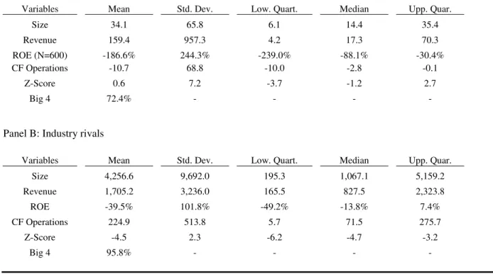
Table 2 provides some descriptive statistics for the announcing and rival firms. On average,
GCO firms are small (mean market capitalization = $34.1 million; mean revenue = $159.4
million), clearly unprofitable (mean ROE = -186.6 percent; median ROE = -88.1 percent)3 and
unable to generate positive cash-flow (mean cash-flow from operations = -$10.7 million; median
cash-flow from operations = -$2.8 million). Not surprisingly, GCO firms are severely distressed
one year in advance of receiving the qualified audit report. The mean Z-score is 0.6, which
indicates a high risk of being forced into bankruptcy in the short-run. Around three-quarters of
the GCO firms are audited by a Big 4 audit firm.
2 With the exception of the years 2001 and 2002 (2001), GCO events are evenly spread over our sample period for the services-prepackaged software industry (services-computer programming, data processing and similar). In untabulated results we drop these two industries/years and rerun our analysis. Our conclusions do not change.
8
The typical industry is much bigger than the individual GCO firm (mean market capitalization
= $4,256.6 million; mean revenue = $1,705.2 million). Industry rivals are also unprofitable
(mean ROE = -39.5 percent) but enjoy a better financial position than that of the GCO firms
(mean cash-flow from operations = $224.9 million). The mean value for our bankruptcy
likelihood proxy is -4.5, suggesting that the typical firm within our industries is not at risk of
failing in the short-term.
III. GCOS STOCK PRICE IMPACT: SHORT-TERM ANALYSIS
In this section, we investigate the short-term valuation effects associated with the disclosure
of a GCO on both the announcing firm and their competitors.
Initial Evidence
We use standard event study methods to explore how GCOs affect market prices. In
particular, for announcing firm j, we compute the abnormal return in day t (ARj t, ) as:
( )
, , ,
j t j t j t
AR =r −E r (1)
9
where rj t, is day t return for the announcing firm j, and E r
( )
j t, is the expected return for suchfirm/trading day. E r
( )
j t, is estimated using the market model. We use the CRSP value weightedportfolio as proxy for the market portfolio, and estimate the parameters of the market model over
a 200 trading-day window, which ends 50 days before the disclosure date of the firm’s GCO
audit report. Moreover, we adjust the estimate for beta as in Scholes and Williams (1977) to
overcome the bias arising from the infrequent trading of financially distressed firms.
Next, for event day t, the average abnormal return (ARt) is defined as:
, 1 1
n
t j t
j
AR n AR
=
=
∑
(2)where ARj t, is as in equation (1) and n is the number of firms. The significance of the average
abnormal return is accessed using Z-statistics computed as in Boehmer et al. (1991).4
We broadly follow Lang and Stulz (1992) when computing the abnormal returns for the
industry rivals. As mentioned in section 2, industry portfolios are comprised of all firms with the
same four-digit SIC code as the announcing firm that have stock returns available on CRPS. To
reduce survival bias, rivals are included in the industry portfolio even if they do not have
reported returns for all days in the estimation or event period.5 Abnormal returns are computed as
prediction errors for the portfolio return, with Lang and Stulz (1992) noting that such procedure
accounts for the cross-sectional dependence among companies in each portfolio. In practice, we
employ equations (1) and (2) with one exception. We do not use the Scholes and Williams
4 Using cross-sectional
t-statistics or Pattel’s (1976) test statistic yields essentially the same results. These are available upon
request from the first author.
10
(1977) adjustment technique as, in this case, the prediction errors are for portfolios of competitor
companies, not the GCO firms’ themselves (see also Haensly et al. 2001). As such, for the rival
portfolios, E r
( )
j t, is estimated using the ordinary least squares (OLS) betas from our marketmodel regression. For completeness, we present results using both equal and value-weighting
schemes for the industry portfolios.
Table 3 summarizes our results. Panel A shows that, on average, the market price of the
announcing firms falls by 1.69 percent (p<0.001) on a risk-adjusted basis at the event date and a
further 1.92 percent (p<0.01) and 1.14% (p=0.035) on event days +1 and +2, respectively. None
of the preevent abnormal returns are statistically significant at conventional levels. Our evidence
is in line with the recent findings of Menon and Williams (2010) and shows that GCOs clearly
provide investors with new and important value-relevant information.
Our original results are, however, reported in panel B of Table 3. As can been seen, the
average abnormal return for both the value-weighted (VW) and equally weighted (EW) rival
portfolios are positive and statistically significant at the event date: 0.37 percent (p<0.001) and
0.24 percent (p=0.023), respectively. Given our results for the announcing firms, such evidence
clearly suggests that the disclosure of a GCO report leads, on average, to an intra-industry
competitive effect, which seems to be driven by the biggest rival firms operating within the
industry.
11
As Lang and Stulz (1992) emphasize, in general, the market capitalization of any individual
firm is considerably smaller than that of its industry. As such, in practice, the relatively small
percentage gain we document for our industry rivals may actually correspond to a very
significant dollar amount. We infer about the economic importance of the GCO competitive
effect assuming that the market value of each of our rival firms (announcing firm) increases
(decreases) by 0.24 percent (1.69 percent) at the GCO disclosure date. Using such conservative
assumption, we estimate the GCO competitive effect to be worth around $171.6 billion (the
announcing firms’ shareholders lose $480 million), in 2009 constant dollars.
In Table 4, we re-examine our results using cumulative abnormal returns (CARs). For each
announcing firm j, the cumulative abnormal return over period τ is:
2
1
, ,
t
j j
t
CAR τ AR τ τ=
=
∑
(3)where ARj t, is defined as in equation (1). Individual CARs for a given time interval τare
averaged cross-sectionally as follows:
, 1 1
n
j j
CARτ n CAR τ
=
=
∑
(4)where CARi,τ is defined as in (3), and n is the number firms.
6 We compute CARs for industry
rivals using a comparable method.
12
In line with the previous literature, panel A of Table 4 shows that GCO firms sustain a
risk-adjusted loss in market value around the audit report disclosure date. In particular, the average
CAR for the announcement period ranges from -1.39 percent (p<0.01) to -3.31 percent (p<0.01),
depending on the event window one considers. The one-week average preevent CAR is not
significant at conventional levels. However, its postevent equivalent is positive and significant at
better than the 1 percent level. Our results thus suggest the market overreacts to the
announcement of a GCO report, with Dawkins et al. (2007) reporting similar evidence for their
sample of bankrupt firms.
In panel B of Table 4, we focus on the rival firms and again show that, on average, the GCO
leads to a competitive effect. The average VW industry CAR for the (-1;0) window is 0.41
percent (p=0.01) and is 0.36 percent (p=0.07) for the more extended (-1;1) period. Results
computed using equal weights are similar, albeit somewhat weaker both statistically and in
magnitude. This supports the idea that the GCO competitive effect is driven by the largest
industry rivals.
Multivariate Evidence
Short-term industry effects may vary significantly due to industry or firm characteristics, as
suggested by Lang and Stulz (1992), Jorion and Zhang (2007) and Zhang (2010) among others.
13
4 3
0 , ,
1 1
i m i m k i k i
m k
CAR α λ Ind δ Firm ε
= =
= +
∑
+∑
+(5)
where CARi is industry i´s CAR over the (-1;0) window, Indi m, represents a set of industry
related characteristics, Firmi k, stands for a set of GCO firm-specific characteristics, and εiis the
error term, assumed to be white noise.7
The first industry characteristic we consider is leverage (Ind_Lev). A priori, the relation
between the GCO competitive effect and industry leverage is ambiguous. On the one hand, all
else being equal, the competitive effect should be more pronounced in highly levered industries.
This is because debt magnifies the impact on return on equity resulting from the (potential)
increase in net earnings accruing to the nonGCO firms. On the other hand, increased leverage
also reduces firms’ ability to invest and, consequently, to exploit changes in their competitive
position (Bolton and Scharfstein 1990). Following Haensly et al. (2001), we compute the ratio of
total debt to total assets at the firm level and then use the industry’s average to estimate equation
(5).8
Concentration is the second industry characteristic we consider (Ind_Conc). In less than fully
competitive industries, an increase in demand should translate into higher equity valuations as
firms can raise the price they charge for their current output. It is plausible that receiving a GCO
leads to a negative reputational effect, which should result in costumers shifting their demand to
nonGCO firms. Consequently, industry concentration should magnify the GCO competitive
7 We use eleven year-dummies and five industry-dummies when estimating equation (5) to overcome potential problems of omitted variables. Industry dummies are defined according to Professor Keneth French’s five industry portfolios.
See http://mba.tuck.dartmouth.edu/pages/faculty/ken.french/Data_Library/det_5_ind_port.html for more details (accessed on 06/09/2011).
14
effect. We use the Herfindahl ratio to proxy for the degree of industry concentration (Lang and
Stulz 1992), which is computed as the squared sum of the fractions of the industry sales by the
nonGCO firms.9
The GCO competitive effect should be smaller (or even inexistent) when the industry shares a
similar cash-flow pattern vis-à-vis that of the announcing firm. Indeed, when this is the case,
investors are less likely to perceive the GCO as being firm-specific, which in turn, should
negatively affect the market price of all the other firms in the industry. Drawing on Lang and
Stulz (1992), we assess the level of cash-flow similarity (Ind_CF) by computing the correlation
between the raw stock returns of the industry and its respective announcing GCO firm over the
one-year period preceding the GCO disclosure date.
Lang and Stulz (1992) mention a potential interaction between industry leverage and
concentration. As argued above, high industry concentration should magnify the intra-industry
GCO competitive effect. However, the extent to which this is actually reflected on stock prices
depends on the industry’s leverage ratio. The average indebtedness of the industry constraints
competitors’ ability to expand their business and influences the response of the return on equity
to fluctuations in market share. Following Haensly et al. (2001), we include an interaction term
between industry leverage and concentration in our regression model to explicitly capture this
joint effect (Lev_Con).
Three GCO firm specific characteristics are also considered in our regression model. The first
is size, which captures the information environment surrounding the announcing firms
(GCO_Size). In a recent paper, Ittonen (2010) shows that size mitigates the negative stock
15
returns associated with the disclosure of an audit report, a result he attributes to the lower levels
of information asymmetry associated with the biggest GCO firms. It follows that investors are
less likely to be surprised by the GCO as the size of the announcing firm increases. This, in turn,
should lead the GCO competitive effect to be concentrated around the smallest announcing
firms. Size is measured as the log of the GCO firm’s total assets, collected from COMPUSTAT
one calendar year before the GCO year.
It is well-established that the market is inefficient when dealing with earnings surprises,
especially when they are negative (Bernard and Thomas 1989, 1990; Fama 1998). This is
important as investors are likely to become aware and react to earnings figures at the same time
they learn about the going concern audit report. Drawing on Foster et al. (1984), we define
earnings surprise as the ratio of the difference of the current quarterly earnings figure and the
earnings figure reported by the firm in the previous quarter to the absolute value of the firm’s
current quarter earnings. We then use a dummy variable (SUE_d) to separate cases where a
positive earnings surprise occurs at the 10k’s disclosure date (dummy equals one) from all the
other cases.
Profitability is the last GCO firm specific variable we consider in equation (5). We proxy for
firm profitability (GCO_ROA) using the return on assets ratio, which we compute as earnings
before interest and taxes to total assets.10 This ratio captures the ability of the firm to use its
assets to generate earnings, with higher values usually indicating increased levels of economic
efficiency and managerial talent. We expect the GCO competitive effect to be stronger when the
16
announcing firm is relatively more profitable as this is akin to saying that a more able competitor
is likely to be forced out of the market shortly.
Panel A of Table 5 presents summary statistics for the independent variables. As can be seen,
on average, our industries do not carry much debt on the balance sheet (mean = 21 percent;
median = 15 percent) and seem relatively concentrated (Ind_Conc for = 0.56; median = 0.50). In
addition, rivals’ preevent raw returns are not strongly correlated with those of the announcing
firm, which suggests that typical event and nonevent firms have distinct assets in place and/or
investment opportunity sets. Panel A of Table 5 again shows that the GCO firms are small, with
mean (median) total assets of $201.4 ($21.9) million and are not profitable, with mean and
median return on assets of -49 percent and -26 percent, respectively. Panel A of Table 5 also
shows that going concern audit reports are very often accompanied by a contemporaneous
negative earnings surprise, emphasizing the need for controlling for the impact of such effect in
our results.
Panel B of Table 5 resumes the Pearson correlation coefficients. The largest is 29.1 percent
for GCO_Size and Ind_CF, (p<0.01) but many are not significant at normal levels. This suggests
that our independent variables proxy for distinct underlying factors and, as such, our regression
results should be free of problems of serious multicollinearity.
Table 6 presents our cross-sectional regression results. We run a Reset test to exclude
problems of incorrectly omitted variables and/or incorrect functional form, and we conduct a
Breush-Pagan and a White test to control for heteroscedasticity. As shown in Table 6, the Reset
test is never significant at normal levels; the opposite holds for the Breush-Pagan and White
17
account for heteroskedasticity. Consequently, and drawing on Lang and Stulz (1992) and
Haensly et al. (2001), we estimate equation (5) using weighted least squares (WLS), with
weights equal to the reciprocal of the standard deviation of the market model residual for the
industry portfolio.11
We now analyze our VW results. Table 6 shows that the coefficient estimated for Ind_Lev and
Ind_Conc is positive and significant while the parallel figure for the interaction term is negative
and significant at better than the 1 percent level. It follows that, ceteris paribus, the GCO
competitive effect for the largest industry rivals is driven by the more highly levered and
concentrated industries. However, for a given level of industry concentration, an increase in the
industry’s average debt ratio mitigates the impact of the GCO on the industry rivals’ market
price. In addition, the coefficient associated with Ind_CF is negative and significant at
conventional levels. Hence, our regression results indicate that similarity of cash-flows between
rivals and announcing firms reduces the magnitude of GCO competitive effect. Table 6 also
shows that the announcing firms’ specific characteristics influence the magnitude of the GCO
competitive effect. In particular, all else being equal, rivals’ abnormal performance around the
GCO date is less negative as the size of the announcing firm increases. In line with our initial
expectations, there is also evidence suggesting that the GCO competitive effect is more acute
when the event firm is relatively more profitable. Finally, Table 6 suggests that a positive
earnings surprise mitigates the intra-industry effect under analysis: the coefficient estimated for
SUE_d is -0.004, with p-value of 0.067.
11 In untabulated results we use two-step generalized least squares (Green, 2002, pp. 227-228) and Ordinary Least Squares (OLS) with heteroskedasticity-robust t-statistics (Zhang 2010) to estimate equation (5). In general, the estimated coefficients have the
18
In general, EW and VW results are largely consistent. There is, however, one important
exception. The coefficient estimated for Ind_Lev and for the interaction term is not significant at
normal levels in our EW regression. This is at odds with our VW evidence and suggests that
industries’ indebtedness is only important for explaining the cross-sectional variation of the GCO
competitive effect for the largest rivals.
Summary
This section shows that GCOs convey important information to the market. Our computations
indicate that, on average, the market price of the announcing firms falls by 1.69 percent on a
risk-adjusted basis at the event date, with a cumulative loss of around 3.31 percent being
document for the full (-1;1) period. Our evidence also suggests that such decline in the stock
price may be an indication of market overreaction since the one-week postGCO average CARs is
positive and significant. Our main contribution, however, is with the pricing implication of
GCOs on the industry rivals. We find that such event leads to a competitive intra-industry effect,
which is both economically and statistically significant and driven by the largest competitors. At
the GCO date, the VW stock price of the industry rivals increases, on average, 0.37 percent on a
risk-adjusted basis, which we conservatively estimate to be worth around $171.6 billion, in 2009
constant dollars.
Further tests show that such intra-industry effect is stronger in more concentrated industries
and when competitors and announcing firms have distinct assets in place and growth
opportunities. Firm-specific characteristics are also important. In particular, the GCO
19
lessened when a positive earnings surprise accompanies the disclosure of the going concern audit
report. Finally, industry leverage seems relevant for explaining the extent of the GCO
competitive effect only in the case of largest industry rivals.
IV. GCOS STOCK PRICE IMPACT: LONGER-TERM ANALYSIS
In an efficient market, the GCO signal should be priced as soon as the audit report becomes
publicly known (Fama 1970). Previous studies, however, show that the market is less then fully
efficient in many situations, and especially so when dealing with public bad news events. For
example, Womack (1996) finds that new sell recommendations are associated with a
post-recommendation drift of -9 percent over a 6-month period. Dichev and Piotroski (2001) show
negative abnormal returns of between -10 percent to -14 percent following Moody’s bond
downgrades in the first year alone, with a further decline of -3 percent to -7 percent in the second
and third years, respectively. In addition, Chan (2003) reports that stocks associated with bad
news stories display a negative drift for up to 12 months.
In a recent paper, Kausar et al. (2009) find that the U.S. market underreacts by no less than
-14 percent over the 12-month period following the disclosure of a GCO report, with Taffler et al.
(2004) reporting similar evidence for the U.K.. These two studies thus suggest the market is
unable to impound on a timely basis the impact of a going concern audit report on the
announcing firm’s market price. This section investigates to what extent a similar anomaly
equally occurs at the industry level.
There is much discussion in the literature regarding long-term event studies. Researchers
20
returns: 1) the calendar time portfolio method (Fama 1998; Mitchell and Stafford 2000), and 2)
the buy-and-hold method (Barber and Lyon 1997). Fama (1998) and Mitchell and Stafford
(2000) argue that event-time returns, as employed by the buy-and-hold method, are an
inappropriate metric for computing long-term abnormal returns since they present cross-sectional
dependence. Barber and Lyon (1997), however, show that the arithmetic summation of returns,
as is done with calendar time returns, does not precisely measure investor experience. Moreover,
Lyon et al. (1999) demonstrate that the calendar time method is generally misspecified in
nonrandom samples, and Loughran and Ritter (2000) show that such technique has low power.
After reviewing the literature, Kothari and Warner (2007) conclude that we still lack an
undisputable method for conducting long-term event studies. Therefore, below we use both the
buy-and-hold and the calendar portfolio methods to examine the longer-term market reaction of
industry rivals to the disclosure of a GCO report.
Buy-and-Hold Risk Adjusted Abnormal Returns
We compute buy-and-hold abnormal returns (BHARs) as Barber and Lyon (1997). In
particular, for period τ, industry i ’s BHAR is given by:
(
)
( )
2 2
1 1
, 1 , 1 ,
t t
i i t i t
t t
BHAR τ r E r
τ= τ=
=
Π
+ −Π
+ (6)
where ri t, is the VW or EW return for industry i at period τ , and E r
( )
i t, is the expected returnfor industry iat period τ . E r
( )
i t, is estimated using the returns of firms matched on size and21
reversion. Our matching procedure is very similar to that of Zhang (2010). In particular, we first
assign each stock present in the CRSP database to one of ten size deciles based on its market
capitalization at the end of June. Next, for each GCO industry firm, we define the control firm as
that firm in the same size decile with the closest book-to-market ratio. Such ratio is computed as
the most recent book value of equity at the end of December divided by the market value of
equity at the end of the same month. Once we identify a control firm for all our GCO industry
firms, we construct both VW and EW portfolios with the returns of the control firms and
generate our measure for E r
( )
i t, . Individual industry BHARs for period τ are then averagedcross-sectionally as follows:
, 1
1 n
i i
BHAR BHAR
n
τ τ
=
=
∑
(7)
where BHARi,τ is defined as in equation (6), and n is the number of industries with data for
period τ. Drawing on Lyon et al. (1999), we compute bootstrapped skewness-adjusted t-statistic
for inferring about the statistical significance of mean BHARs.12,13 A month is defined as a
twelve 21-trading day interval (Michaely et al. 1995), and we restrict our analysis to a one-year
postevent period as considering longer horizons is methodologically challenging (Brown and
Warner 1980; Lyon et al. 1999; Kothari and Warner 2007). For completeness, we also compute
BHARs for the announcing firms using essentially the same procedure as for the industry rivals.
Table 7 presents our results. Panel A summarizes the preevent stock abnormal performance
and shows that, on average, the VW (EW) industry portfolio loses 9.3 percent (p<0.01) (9.6
12 We winsorize our results at the top and bottom 1% to reduce the impact of extreme observation in our results. 13 Standard cross-sectional
22
percent; p<0.01) of its market value on a risk-adjusted basis over the one-year period preceding
the GCO announcement date. Results for the six-month preevent period are qualitatively similar,
although of smaller magnitude. Furthermore, panel A of Table 7 shows that, on average, the
GCO firms earn significant and negative risk-adjusted returns over the same two compounding
windows (74.4 percent for the one-year period and 43.9 percent for the six-month period). Taken
together, our results suggest the market suspects of the future prospects of both the announcing
firms and their industry rivals before the GCO disclosure date.
Panel B of Table 7, however, shows a different pattern in the postevent period. In particular,
the (2, 21) mean VW and EW industry BHARs are positive and significant (1.5 percent and 1.9
percent respectively), while most of their longer-term equivalents are not significant at normal
levels. The converse occurs with the GCO firms, with the mean abnormal return for the first
postGCO month not statistically significant but all the others strongly negative and significant.
These results suggest the market prices the announcing firms and their industry rivals differently
once the audit report is disclosed. In particular, there is evidence that GCO firms’ shareholders
(continue to) lose value on a risk-adjusted basis in the postGCO period whereas investors in their
industry rivals earn positive abnormal returns in the first postGCO month.
Calendar-time Portfolios
As mentioned above, Fama (1998) and Mitchell and Stafford (2000) highlight some potential
pitfalls with the BHAR method, and favor the use of calendar-time portfolios. For robustness, we
also employ this alternative method focusing on the rival firms (see also Eberhart et al. 2004 and
23
data collected from the CRSP monthly database. Each GCO industry is included in a
rolling-calendar portfolio at the GCO report disclosure month, and is hold there up to a maximum of 6-
or 12-months.14 Industries are given the same weight in the calendar portfolio in all months
(Zhang 2010), and following Mitchell and Stafford (2000) and Ikenberry and Ramnath (2002),
we drop all months where the calendar portfolio has fewer than 10 industries.
The calendar portfolio abnormal performance is assessed using the Fama and French’s (1993)
three- and the Carhart’s (1997) four-factor model. We use a Breush-Pagan and a
Breusch-Godfrey serial correlation LM test to check for heteroskedasticity and autocorrelation,
respectively. The Breush-Pagan test is never significant, an indication that heteroskedasticity is
not an issue. However, the LM test suggests that serial correlation is present in almost all of our
regressions using VW industry returns. As such, below we present OLS t-statistics corrected for
autocorrelation when appropriate.
Table 8 summarizes our findings. In panel A we examine what happens before the
announcement of the going concern audit report. As can be seen, all VW intercepts are negative
and significant. While the results for the EW industry returns are similar, they are not statistically
significant when one considers the 12-month holding period. However, in general, there is
evidence to conclude that our calendar time results suggest that the industry rivals lose value on a
risk-adjusted basis in the preGCO period. Panel B of Table 8 presents the postevent results,
which are in line with the BHAR evidence reported above. In particular, we find that most
intercepts are not statistically significant at normal levels, which implies that, in the longer-run,
one cannot earn risk-adjusted excess returns by investing in the GCO firm’s industry rivals.
24
Overall, this section shows that GCO firms and their competitors experience negative and
significant returns in the one-year period preceding the publication of a going concern opinion.
However, postevent, such return pattern changes and critically depends on whether the auditor
qualifies the firm or not. In particular, we find that GCO firms continue to lose market value
within the one-year period following the announcement date whilst their rivals earn positive
abnormal returns in the subsequent month.
V. CONCLUSION
We use a large sample of 670 firms receiving a going concern opinion in the U.S. between
1994 and 2005 and show that such accounting event helps investors adjust their expectations
about the future prospects of both the announcing firms and their industry rivals. In particular, in
the preevent period, all firms in the industry lose value on a risk-adjusted basis. We observe an
intra-industry competitive effect at the GCO disclosure date as rivals (GCO firms) earn average
excess returns of 0.37 percent (-1.69 percent). Postevent, we find that the announcing firms
continue to exhibit negative mean excess returns over the one-year window following the GCO
date whereas buying-and-holding their industry competitors, on average, yields positive
abnormal returns in the first postGCO month.
Our evidence adds to the literature in two important ways. First, we show that GCOs clearly
have market pricing implications for industry rivals. This constitutes an original contribution as
the previous studies typically focus on the announcing firms. Second, we demonstrate the market
25
they suggest such accounting event is bad news for the GCO firms yet good news for their
industry rivals.
REFERENCES
Aharony, J., and I. Swary. 1983. Contagion effects of bank failures: evidences from capital markets. Journal of
Business 56 (3): 305-322.
Ball, R., and P. Brown. 1968. An empirical evaluation of accounting income numbers. Journal of Accounting
Research 6 (2): 159-167.
Barber, B., and J. Lyon. 1997. Detecting long-run abnormal stock returns: the empirical power and specification of test statistics. Journal of Financial Economics 43 (3): 341-372.
Bernard, V., and J. Thomas. 1989. Post-earnings announcement drift: delayed price response or risk premium? Journal of Accounting Research 27 (3): 37-48.
Bernard, V., and J. Thomas. 1990. Evidence that stock prices do not fully reflect the implications of current earnings for future earnings. Journal of Accounting and Economics 13(4): 305-340.
Boehmer, E., J. Musumeci and, A. Poulsen. 1991. Event-study methodology under conditions of event-induced variance. Journal of Financial Economics 30 (2): 253-272.
Bolton, P., and D. Scharfstein. 1990. A theory of predation based on agency problems in financial contracting. American Economic Review 80 (1): 93-106.
Brown, S., and J. Warner. 1980. Measuring security price performance. Journal of Financial Economics 8 (3): 205-258.
Carhart, M. 1997. On persistence in mutual fund performance. Journal of Finance 52 (1): 57-82.
Chan, W. 2003. Stock price reaction to news and no-news: drift and reversal after headlines. Journal of Financial Economics 70 (2): 223-260.
Dawkins, M., N. Bhattacharya, and L. Bamber. 2007. Systematic share price fluctuations after bankruptcy filings and the investors who drive them. Journal of Financial and Quantitative Analysis 42 (2): 399-420.
Dichev, I., and J. Piotroski. 2001. The long-run stock returns following bond rating changes. Journal of Finance 56 (1): 173-203.
Eberhart, A., M. William, and A. Siddique. 2004. An examination of long-term abnormal stock returns and operating performance following R&D increases. Journal of Finance 59 (2): 623-650.
Elliot, R., M. Highfield, and M. Schaub. 2006. Contagion or competition: Going concern audit opinions for real estate firms. Journal of Real Estate Finance and Economics 32 (4): 435-448.
26
Fama, E. 1970. Efficient capital markets: a review of theory and empirical work. Journal of Finance 25 (2): 383-417.
Fama, E. 1998. Market efficiency, long-term returns, and behavioral finance. Journal of Financial Economics 49
(3): 283-306.
Fama, E., and K. French. 1993. Common risk factors in the returns on stocks and bonds. Journal of Financial
Economics 33 (1): 3-56.
Fleak, K., and E. Wilson. 1994. The incremental information content of going-concern audit opinion. Journal of
Accounting, Auditing and Finance 9 (1): 149-166.
Foster, G., C. Olsen, and T. Shevlin. 1984. Earnings releases, anomalies and the behavior of security returns. The Accounting Review 59 (4): 574-603.
Gay, G., S. Timme, and K. Yung. 1991. Bank failure and contagion effects: evidence from Hong Kong. Journal of Financial Research 14 (2): 153-168.
Greene, W. 2002. Econometric Analysis. 5th edn, New Jersey: Prentice Hall.
Haensly, P., J. Theis, and Z. Swanson. 2001. Reassessment of contagion and competitive intra-industry effects of bankruptcy announcements. Quarterly Journal of Business and Economics 40 (3): 45-63.
Ikenberry, D., and S. Ramnath. 2002. Underreaction to self-selected news events: The case of stock splits. Review of Financial Studies 15 (2): 489-526.
Ittonen, K. 2010. Information asymmetries and investor reactions to going concern audit reports. Working paper. Available at SSRN: http://ssrn.com/abstract=1698595.
Jones, F.1996. The information content of the auditor's going-concern evaluation. Journal of Accounting and Public Policy 15 (1): 1-27.
Jorion, P., and G. Zhang. 2007. Good and bad credit contagion: Evidence from Credit Default Swaps. Journal of Financial Economics 84 (3): 860-883.
Jorion, P., and G. Zhang. 2010. Information transfer effects of bond rating downgrades. Financial Review 45 (3): 683-706.
Kausar, A., R. Taffler, and C. Tan. 2009. The going-concern market anomaly. Journal of Accounting Research, 47 (1): 213-239.
Kothari, S., and J. Warner. 2007. Econometrics of Event Studies. In Handbook of Corporate Finance: Empirical Corporate Finance, Volume 1, edited by B. Espen Eckbo, 3-32. Holland: Elsevier.
Lang, L., and R. Stulz. 1992. Contagion and competitive intra-industry effects of bankruptcy announcements: an empirical analysis. Journal of Financial Economics 32 (1): 45-60.
Loughran, T., and J. Ritter. 2000. Uniformly least powerful tests of market efficiency. Journal of Financial
Economics 55 (3): 361-389.
27
Menon, K., and D. Williams. 2010. Investor reaction to going concern audit reports. The Accounting Review 85 (6): 2075-2105.
Michaely, R., R. Thaler, and K. Womack. 1995. Price reactions to dividend initiations and omissions: overreaction or drift? Journal of Finance 50 (2): 573-608.
Mitchell, M., and E. Stafford. 2000. Managerial decisions and long-term stock price performance. Journal of
Business 73 (3): 287-329.
Ogneva, M., and K. Subramanyam. 2007. Does the stock market underreact to going-concern opinions? Evidence from the US and Australia. Journal of Accounting and Economics 43 (2-3): 439-452.
Patell, J. 1976. Corporate forecasts of earnings per share and stock price behavior: Empirical tests. Journal of
Accounting Research 14 (2): 246–276.
Schaub, M. 2006. Investor reaction to regulated monopolies announcing going concern opinions - What explains contagion among electric services companies? Review of Accounting and Finance 5 (4): 393-409.
Schaub, M., M. Watters, and G. Linn. 2003. Going concern opinions useful in conveying information regarding the computer industry and firms. Academy of Accounting and Financial Studies Journal 7 (3): 11-19.
Scholes, M., and J. Williams. 1977. Estimating betas for nonsynchronous data. Journal of Financial Economics 5 (3): 309-327.
Taffler, R., J. Lu, and A. Kausar. 2004. In denial? Stock market underreaction to going-concern audit report disclosures. Journal of Accounting and Economics 38: 263-296.
Womack, K. 1996. Do brokerage analyst's recommendations have investment value? Journal of Finance 51 (1):
137-167.
Zhang, G. 2010. Emerging from Chapter 11 bankruptcy: Is it good news or bad news for industry competitors? Financial Management 39 (3): 1719-1742.
28
Table 1
Sample Selection and Distribution by Year
This table summarizes the sample construction strategy and the distribution of cases by year. Panel A: Sample selection
We start by identifying on EDGAR all 10k reports that mention the words “raise substantial doubt” and “ability to continue as a going concern” between 01/01/1994 and 12/31/2005. Conditional on a firm having data in the CRSP/COMPUSTAT merged database, we manually verify if the company has a GCO audit report in that fiscal year and if the previous fiscal year is clean in order to identify the first-time GCO companies. We then exclude all cases that filed Chapter 11 before the audit report publication date, all firms classified as foreign or as development stage enterprise, and cases with insufficient CRSP/COMPUSTAT data. Next, utilities and financials are deleted. Finally, we exclude all GCO cases for which we cannot find at least one industry rival (defined as having the same four-digit SIC CODE) on COMPUSTAT and/or the industry rivals do not have return data available on the CRSP daily file.
Sample Frequency
Firm-year observations identified through 10k wizard 29,102 Firm-year observations not found in CRSP/Compustat merged 16,866 Firm-year observations that do not constitute First-time GCM 9,940 Firm-year observations with insufficient CRSP/COMPUSTAT data 1,017 Firm-year observations classified as utilities or financials 142 Firm-year observations classified as foreign or as in a development stage 168 Firm-year observations filing Chapter 11 before audit report publication date 45 Firm-year observations without at least one valid industry rival 254
Final sample size 670
Panel B: Sample Distribution by Year
Year Frequency Percentage
1994 15 2.2%
1995 37 5.5%
1996 49 7.3%
1997 68 10.1% 1998 68 10.1% 1999 70 10.4%
2000 48 7.2%
2001 95 14.2% 2002 101 15.1% 2003 69 10.3%
2004 22 3.3%
2005 28 4.2%
29
Table 2 Summary statistics
This table presents summary statistics relating to the GCO firms and their industry rivals. Industry rivals are defined as firms sharing the same 4-digit SIC code as the announcing firm and that have data available on both CRSP and COMPUSTAT. Size is the equity market capitalization in $m, measured one month before the GCO date. Revenue is total revenues in $m. ROE is the return on equity, computed as the ratio of net income to book value of equity. CF Operations is the cash-flow from operations in $m. Z-score is a composite measure of financial distress based on Zmijewski (1984). Big 4 is a dummy that assumes the value 1 if the firm is audited by a Big 4 audit firm or one of its predecessors and zero otherwise. All accounting data is collected from the 10k report disclosed one year before the GCO announcement date.
Panel A: GCO firms
Variables Mean Std. Dev. Low. Quart. Median Upp. Quar.
Size 34.1 65.8 6.1 14.4 35.4
Revenue 159.4 957.3 4.2 17.3 70.3
ROE (N=600) -186.6% 244.3% -239.0% -88.1% -30.4% CF Operations -10.7 68.8 -10.0 -2.8 -0.1
Z-Score 0.6 7.2 -3.7 -1.2 2.7
Big 4 72.4% - - - -
Panel B: Industry rivals
Variables Mean Std. Dev. Low. Quart. Median Upp. Quar. Size 4,256.6 9,692.0 195.3 1,067.1 5,159.2 Revenue 1,705.2 3,236.0 165.5 827.5 2,323.8 ROE -39.5% 101.8% -49.2% -13.8% 7.4% CF Operations 224.9 513.8 5.7 71.5 275.7
Z-Score -4.5 2.3 -6.2 -4.7 -3.2
30
Table 3
Abnormal returns associated with GCO announcements
This table presents the short-term industry effect associated with GCOs. The abnormal return (AR) is the market model residual (estimated over the -250, -50 day interval). The sample includes all GCOs between 01/01/1994 and 12/31/2005 for which a primary 4-digit SIC code is available from the COMPUSTAT data file (670 GCOs). An industry portfolio is a value-weighted (VW) or an equally weighted (EW) portfolio of firms with the same primary 4-digit SIC code for which returns are available from the CRPS files. N denotes the number of abnormal returns to compute the average abnormal return. The significance of the AR is computed as in Boehmer et al. (1991).
Panel A: Announcing firms’ average abnormal returns around the GCO announcement date
Event Day N Mean Sign. -5 669 0.40% 0.505
-4 668 0.29% 0.802
-3 668 -0.38% 0.283
-2 668 0.12% 0.835
-1 668 0.30% 0.497
0 666 -1.69% 0.000
1 667 -1.92% 0.000
2 669 -1.14% 0.035
3 669 0.81% 0.152
4 669 1.98% 0.013
5 668 0.65% 0.100
Panel B: Industry rivals’ average abnormal returns around the GCO announcement date
Event Day N VW Mean VW Sign. EW Mean EW Sign. -5 670 0.03% 0.769 0.07% 0.797
-4 670 0.22% 0.193 0.15% 0.351
-3 670 0.21% 0.348 0.35% 0.001
-2 670 0.01% 0.557 0.12% 0.148
-1 670 0.15% 0.209 0.13% 0.448
0 670 0.37% 0.008 0.24% 0.023
1 670 -0.01% 0.587 -0.01% 0.650
2 670 0.14% 0.112 0.00% 0.908
3 670 0.20% 0.008 0.09% 0.183
4 670 -0.16% 0.054 -0.11% 0.179
31
Table 4
Cumulative abnormal returns associated with GCO announcements
This table presents the cumulative short-term industry effect associated with the disclosure of GCO report. The cumulative abnormal return (CAR) is the market model residual (estimated over the -250, -50 day interval) in. The sample includes all GCOs between 01/01/1994 and 12/31/2005 for which a primary 4-digit SIC code is available from the COMPUSTAT data file (670 GCOs). An industry portfolio is a value-weighted (VW) or an equally weighted (EW) portfolio of firms with the same primary 4-digit SIC code for which returns are available from the CRPS files. N denotes the number of abnormal returns to compute the average abnormal return. The significance of the AR is computed as in Boehmer et al. (1991).
Panel A: Announcing firms’ average cumulative abnormal returns
Period N Mean Sign. (-6; -2) 669 0.03% 0.639
(-1; 0) 668 -1.39% 0.005
(-1; 1) 668 -3.31% 0.000
(2; 6) 670 3.37% 0.002
Panel B: Industry rivals’ average cumulative abnormal returns
Period N VW Mean VW Sign. EW Mean EW Sign. (-6; -2) 670 0.34% 0.136 0.47% 0.021
(-1; 0) 670 0.41% 0.010 0.23% 0.091
(-1; 1) 670 0.36% 0.066 0.14% 0.428
32
Table 5
Summary statistics of independent variables
This table presents descriptive statistics for the independent variables used to explore the determinants of the short-term industry effect associated with the disclosure of a GCO report. Panel A reports the summary statistics for such variables, and Panel B presents the Pearson correlation coefficients. Ind_Lev is measures the industry’s level of indebtedness (total debt to total assets). Ind_Conc is the Herfindahl ratio, computed as the squared sum of the fractions of the industry sales (higher values indicate a more concentrated industry). Ind_CF is a proxy for the degree of similarity in cash flows between the industry and the announcing firm (measured as the coefficient of correlation of raw returns over the one year period preceding the event date). LGCO_Size is the announcing firm’s log of total assets (in $m, computed with data collected from the 10k report disclosed one year prior to the GCO report date) and is used to capture the information environment surrounding the event firms. GCO_ROA is the ratio of earnings before earnings and taxes to total assets and measures the pre-event profitability of the announcing firm. SUE_d is a dummy variable assuming the unit value the GCO report is accompanied by a positive earnings surprise, and zero otherwise. P-values are presented in parentheses.
Panel A: Summary statistics
Variable Mean StdDev Min Median Max Ind_Lev 0.21 0.16 0.00 0.15 0.72 Ind_Conc 0.56 0.29 0.13 0.50 1.00 Ind_CF 0.08 0.12 -0.26 0.06 0.70 LGCO_Size 201.43 1484.00 0.66 21.9 30267.00 GCO_ROA -0.49 0.67 -5.90 -0.26 0.38
SUE_d 0.4 0.5 0 0 1
Panel B: Correlation table
Variable Ind_Lev Ind_Conc Ind_CF GCO_Size GCO_ROA SUE_d
Ind_Conc 0.131 1.000
(0.001)
Ind_CF -0.099 -0.263 1.000
(0.010) (<.0001)
GCO_Size 0.144 -0.032 0.291 1.000
(<.0001) (0.402) (<.0001)
GCO_ROA 0.290 0.168 -0.070 0.077 1.000
(<.0001) (<.0001) (0.072) (0.047)
SUE_d -0.114 -0.024 -0.057 -0.060 -0.202 1.000
(0.003) (0.529) (0.141) (0.123) (<.0001)
33
Table 6
Cross-sectional analysis of industry rival’s short-term abnormal equity returns
This table presents the coefficient estimates of cross-section regressions for the short-term industry abnormal returns for a sample of 670 events. The dependent variable is the cumulative abnormal stock returns for the industry portfolio from a market model for the (-1,+0) daily interval, where Day 0 is the disclosure of the GCO report. Ind_Lev is measures the industry’s level of indebtedness (total debt to total assets). Ind_Conc is the Herfindahl ratio, computed as the squared sum of the fractions of the industry sales (higher values indicate a more concentrated industry). Ind_Lev_Conc is an interaction variable, computed as Ind_Lev times Ind_Conc. Ind_CF is a proxy for the degree of similarity in cash flows between the industry and the announcing firm (measured as the coefficient of correlation of raw returns over the one year period preceding the event date). LGCO_Size is the announcing firm’s log of total assets (in $m, computed with data collected from the 10k report disclosed one year prior to the GCO report date) and is used to capture the information environment surrounding the event firms. GCO_ROA is the ratio of earnings before earnings and taxes to total assets and measures the pre-event profitability of the announcing firm. SUE_d is a dummy variable assuming the unit value the GCO report is accompanied by a positive earnings surprise, and zero otherwise. An industry portfolio is a value-weighted (VW) or an equally weighted (EW) portfolio of firms with the same primary 4-digit SIC code for which returns are available from the CRPS files. Models are estimated using weighted least squares and include both year and industry dummies.
VW EW
Independent Variable Estimate Sig. Estimate Sig. Intercept -0.031 <.001 -0.021 0.001
Ind_Lev 0.089 <.001 -0.015 0.221
Ind_Conc 0.026 <.001 0.009 0.077 Ind_Lev_Conc -0.115 <.001 0.014 0.478 Ind_CF -0.021 0.053 -0.039 0.001 LGCO_Size -0.002 0.003 0.002 0.630 GCO_ROA 0.003 0.068 0.006 0.001 SUE_d -0.004 0.067 -0.005 0.024
Reset (F-Stat. Sig.) 0.546 0.386
White (F-Stat. Sig.) <.0001 <.0001
B.-P. (F-Stat. Sig.) <.0001 <.0001
R-Squared 26.8% 23.2%
34
Table 7
Longer-term industry abnormal equity returns associated with GCO announcements
This table presents long-term abnormal equity returns for the industry portfolios and announcing firms for the sample of 670 GCO events using the size and book-to-market matched model (SBMM). The SBMM calculates the abnormal equity returns for a value-weighted (VW) or equally weighted (EW) industry portfolio in excess of the returns of a value-weighted (VW) or equally weighted portfolio (EW) matching portfolio constructed with size and book-to-market firms. The match firm is in the same size decile as the firm in the industry portfolio and has the closest book-to-market ratio. Panel A (B) reports the average SBMM BHARs for the preevent (postevent) period. P-values are computed using bootstrapped skewness-adjusted t-statistics as in Lyon et al. (1999).
Panel A: Preevent returns
VW EW GCO firms
Period Mean Sign. Mean Sign. Mean Sign. (-252; -2) -0.093 <0.001 -0.096 <0.001 -0.744 <0.001
(-126; -2) -0.035 0.032 -0.027 0.071 -0.439 <0.001
Panel B: Postevent returns
VW EW GCO firms
Period Mean Sign. Mean Sign. Mean Sign. (2; 21) 0.015 0.036 0.019 0.001 -0.003 0.831
(2; 63) 0.013 0.262 0.013 0.018 -0.079 0.002
(2; 126) 0.003 0.851 0.025 0.121 -0.138 <0.001
(2; 189) 0.008 0.710 0.073 0.112 -0.166 <0.001
35
Table 8
Longer-term industry abnormal equity returns associated with GCO announcements - robustness
This table presents long-term abnormal equity returns for the industry portfolios for the sample of 670 GCO events using the calendar-time portfolio model. An industry portfolio is a value-weighted (VW) or an equally weighted (EW) portfolio of firms with the same primary 4-digit SIC code for which returns are available from the CRPS files. Industries are added to the calendar portfolio at the GCO disclosure month and held for 6- or 12-months. Portfolio returns are computed assuming an equally weighted investment strategy. Months where the portfolio holds less than 10 stocks are deleted. The abnormal performance of the industry portfolio is assessed using Fama and French’s (1993) three-factor and Carhart’s (1997) four-factor model. The parameters are estimated using OLS. The p-value of
standard (autocorrelation robust) t-statistics is reported in parentheses (brackets). N is the number of calendar
portfolios considered in the estimation. Panel A: Preevent returns
Value-Weighted industry returns
Holding Period N Intercept Sig. R2 Pricing model 6 Months 119 -0.0028 [<.001] 71.0% Carhart 6 Months 119 -0.0027 [<.001] 71.6% FF 12 Months 140 -0.0024 [<.001] 62.3% Carhart 12 Months 140 -0.0025 [<.001] 62.0% FF
Equally Weighted industry returns
Holding Period N Intercept Sig. R2 Pricing model 6 Months 119 -0.0096 (<.001) 86.0% Carhart 6 Months 119 -0.0048 (0.016) 81.3% FF 12 Months 140 0.0030 (0.206) 88.2% Carhart 12 Months 140 -0.0001 (0.962) 84.4% FF
Panel B: Postevent returns
Value-Weighted industry returns
Holding Period N Intercept Sig. R2 Pricing model 6 Months 119 -0.0017 (0.654) 56.7% Carhart 6 Months 119 -0.0017 (0.226) 56.9% FF 12 Months 140 -0.0031 [0.452] 48.8% Carhart 12 Months 140 -0.0032 [0.314] 71.7% FF
Equally Weighted industry returns