José Maria Pantoja Mata Vale e Azevedo
Licenciado em Engenharia InformáticaImage Stream Similarity Search in GPU Clusters
Dissertação para obtenção do Grau de Mestre em Engenharia Informática
Orientador: Hervé Paulino, Assistant Professor, Faculdade de Ciências e Tecnologia da Universidade Nova de Lisboa Co-orientador: João Magalhães, Assistant Professor,
Faculdade de Ciências e Tecnologia da Universidade Nova de Lisboa
Júri
Presidente: Doutor João M. S. Lourenço
Image Stream Similarity Search in GPU Clusters
Copyright © José Maria Pantoja Mata Vale e Azevedo, Faculdade de Ciências e Tecnologia, Universidade NOVA de Lisboa.
A Faculdade de Ciências e Tecnologia e a Universidade NOVA de Lisboa têm o direito, perpétuo e sem limites geográficos, de arquivar e publicar esta dissertação através de exemplares impressos reproduzidos em papel ou de forma digital, ou por qualquer outro meio conhecido ou que venha a ser inventado, e de a divulgar através de repositórios científicos e de admitir a sua cópia e distribuição com objetivos educacionais ou de inves-tigação, não comerciais, desde que seja dado crédito ao autor e editor.
Este documento foi gerado utilizando o processador (pdf)LATEX, com base no template “novathesis” [1] desenvolvido no Dep. Informática da FCT-NOVA [2].
A c k n o w l e d g e m e n t s
I am grateful for my advisers, Prof. Doutor Hervé Paulino and Prof. Doutor João Maga-lhães for their continued support throughout the conception, research and elaboration of this thesis. I am thankful for the great institution that is FCT/UNL, its professors, employees and fellow students. They provided me with the best education I could hope for, and granted me tools that I am sure will use throughout my whole life. I could not be more happy that I frequented this institution, and these are five years I am sure will never forget.
I would like to thank my father, Álvaro Vale e Azevedo, who constantly inspires and enables me to become the best engineer possible, following his footsteps. I would also like to thank my mother, Joana Pantoja Mata, because without her insistence and concern for my future, I wouldn’t be half the student I am. I could not be more grateful for the parents I have, who worked hard their whole life, and sacrificed time of their own to see me achieve success.
A b s t r a c t
Images are an important part of today’s society. They are everywhere on the inter-net and computing, from news articles to diverse areas such as medicine, autonomous vehicles and social media. This enormous amount of images requires massive amounts of processing power to process, upload, download and search for images. The ability to search an image, and find similar images in a library of millions of others empowers users with great advantages. Different fields have different constraints, but all benefit from the
quick processing that can be achieved.
Problems arise when creating a solution for this. The similarity calculation between several images, performing thousands of comparisons every second, is a challenge. The results of such computations are very large, and pose a challenge when attempting to process. Solutions for these problems often take advantage of graphs in order to index images and their similarity. The graph can then be used for the querying process. Creating and processing such a graph in an acceptable time frame poses yet another challenge.
In order to tackle these challenges, we take advantage of a cluster of machines equipped with Graphics Processing Units (GPUs), enabling us to parallelize the process of describ-ing an image visually and finddescrib-ing other images similar to it in an acceptable time frame. GPUs are incredibly efficient at processing data such as images and graphs, through
al-gorithms that are heavily parallelizable. We propose a scalable and modular system that takes advantage of GPUs, distributed computing and fine-grained parallellism to detect image features, index images in a graph and allow users to search for similar images.
The solution we propose is able to compare up to 5000 images every second. It is also able to query a graph with thousands of nodes and millions of edges in a matter of milliseconds, achieving a very efficient query speed. The modularity of our solution
allows the interchangeability of algorithms and different steps in the solution, which
provides great adaptability to any needs.
R e s u m o
As imagens são uma parte vital da sociedade actual. Existem em todo o lado na internet e na computação, desde artigos de notícias a áreas tão diversas como a medicina, veículos autónomos e redes sociais. Esta quantidade enorme de imagens necessita de um poder de processamento suficiente para as processar. A possibilidade de pesquisar uma imagem e encontrar imagens semelhantes a qualquer outra, permite a utilizadores de variadas áreas navegar as grandes quantidades de dados que existem, de uma forma rápida e fácil. Algumas áreas têm requisitos diferentes, contudo todas beneficiam do rápido processamento que pode ser alcançado.
Diversos problemas ocorrem ao criar uma solução para estes desafios. O cálculo de semelhança entre diversas imagens, e a execução de milhares de comparações a cada segundo, é um desafio. Os resultados de computações como estas são extremamente grandes, e criam um desafio de processamento. Soluções para estes problemas tipicamente usam grafos com o intuito de indexar imagens e a sua semelhança. O grafo pode então ser usado para o processo de pesquisa. A criação e processamento de um grafo deste tipo apresenta ainda outro desafio.
De forma a solucionar estes desafios, tiramos partido de umclusterde máquinas equi-padas com Unidades de Processamento Gráficos (do inglês Graphics Processing Unit, GPU), que nos permite paralelizar o processo de descrever uma imagem visualmente e encontrar outras imagens semelhantes numa janela de tempo aceitável. Os GPUs são ex-tremamente eficientes a processar dados tais como imagens e grafos, através de algoritmos extremamente paralelizáveis. Propomos um sistema escalável e modular que, através dos benefícios dos GPUs, da computação distribuída e do paralelismo de grão fino, detecta características visuais em imagens, indexa-as num grafo e permite que os utilizadores procurem por imagens semelhantes.
C o n t e n t s
List of Figures xvii
List of Tables xix
1 Introduction 1
1.1 Motivation . . . 1
1.2 Problem. . . 2
1.3 Solution . . . 3
1.3.1 Execution Model . . . 4
1.4 Contributions . . . 7
1.5 Document Structure. . . 8
2 State of the Art 9 2.1 GPU Architecture and Programming . . . 9
2.1.1 NVIDIA Architecture . . . 10
2.1.2 Programming: CUDA. . . 12
2.2 Image Feature Detection and Description on GPUs . . . 15
2.2.1 OpenCV . . . 15
2.2.2 Histogram of Oriented Gradients . . . 16
2.2.3 Scale-Invariant Feature Transform . . . 17
2.2.4 Speeded-Up Robust Features . . . 18
2.2.5 Features from Accelerated Segment Test . . . 19
2.2.6 Vector of Locally Aggregated Descriptors . . . 20
2.2.7 Deep Learning Visual Features . . . 20
2.2.8 Binary Robust Independent Elementary Features . . . 20
2.2.9 Oriented FAST and Rotated BRIEF . . . 21
2.2.10 Preliminary Benchmark . . . 21
2.3 Feature Matching . . . 23
2.3.1 k-Nearest Neighbours. . . 23
2.3.2 GPU-Accelerated k-Nearest Neighbours . . . 25
2.4 GPU Graph Processing . . . 26
2.4.1 Solutions . . . 26
2.4.3 GunRock . . . 28
2.4.4 Conclusion . . . 29
2.5 Distributed Stream Processing . . . 29
2.5.1 Apache Storm . . . 30
2.5.2 Intel Threading Building Blocks. . . 31
2.6 Multimedia Stream Processing in GPU Clusters . . . 32
3 Similarity Search 35 3.1 System Description . . . 35
3.1.1 Feature Extraction. . . 36
3.1.2 Feature Matching Algorithms . . . 38
3.1.3 Time Comparison . . . 39
3.1.4 Input: Image Stream . . . 39
3.1.5 Output: SS Graphs . . . 39
3.1.6 Operations . . . 40
3.2 System Architecture . . . 41
3.2.1 Feature Extractor Role . . . 42
3.2.2 Feature Matcher Role . . . 43
4 System Implementation 45 4.1 Technologies used . . . 46
4.1.1 OpenCV . . . 46
4.1.2 Threading Building Blocks . . . 46
4.1.3 Google Protocol Buffers . . . . 48
4.1.4 Gunrock . . . 48
4.1.5 cURL . . . 49
4.1.6 Boost . . . 49
4.2 The SS Image Datastructure . . . 49
4.3 The SS Graph Datastructure . . . 50
4.3.1 Matrix-market coordinate format . . . 50
4.4 Image Processing Workflow . . . 51
4.4.1 Source Node . . . 52
4.4.2 GPU Load Node . . . 53
4.4.3 Image Info Save Node. . . 53
4.4.4 Time Load Node. . . 54
4.4.5 Time Comparison Node . . . 54
4.4.6 Feature Extraction Node . . . 55
4.4.7 Feature Save Node . . . 56
4.4.8 Indexer Node . . . 56
4.4.9 Feature Matching Node. . . 57
CO N T E N T S
4.5 Query Workflow . . . 58
4.6 Conclusion . . . 59
5 System Evaluation 61 5.1 Metrics . . . 61
5.2 Application. . . 62
5.2.1 Application input: the YFCC100M Dataset . . . 62
5.2.2 Algorithms and Parameters . . . 63
5.2.3 SURF Parameters . . . 63
5.2.4 HOG Parameters . . . 64
5.2.5 ORB Parameters . . . 64
5.3 Hardware and Configuration. . . 65
5.4 Single Algorithm Tests and Results . . . 67
5.4.1 Feature Extraction with persistence enabled . . . 67
5.4.2 Feature Matching with persistence enabled . . . 72
5.4.3 Feature Extraction with persistence disabled . . . 73
5.4.4 Feature Matching with persistence disabled . . . 78
5.4.5 Summary. . . 79
5.5 All Algorithms Tests and Results . . . 81
5.5.1 Pipeline steps comparison . . . 83
5.5.2 Summary. . . 85
5.6 Comparison with CPU Implementation. . . 85
5.6.1 Feature Extraction. . . 86
5.6.2 Feature Matching . . . 88
5.6.3 Summary. . . 93
5.7 Query Tests and Results . . . 93
5.7.1 Query precision evaluation . . . 96
5.8 Summary . . . 100
6 Conclusion and Future Work 105 6.1 Conclusion . . . 105
6.2 Future work . . . 106
L i s t o f F i g u r e s
1.1 Distributed Pipeline . . . 6
1.2 Example graph . . . 7
2.1 CPU vs GPU cores . . . 10
2.2 Pascal microarchitecture GPU, taken from [34]. . . . 11
2.3 Pascal streaming multiprocessor, taken from [34]. . . . 12
2.4 CUDA Thread Hierarchy . . . 13
2.5 CUDA Execution Model . . . 14
2.6 HOG Visual Features . . . 16
2.7 HOG Histogram . . . 17
2.8 SIFT Key points. . . 18
2.9 FAST Keypoints. . . 19
2.10 k-NN Illustration . . . 24
2.11 Brute-force matching with k-NN . . . 24
2.12 Bolts and Sprouts Topology . . . 30
2.13 Serial Execution . . . 31
2.14 Parallel Execution . . . 32
3.1 Similarity Search top-level Flow Graph . . . 36
3.2 Similarity Search Architecture . . . 42
3.3 Feature Extractor Flow . . . 43
3.4 Feature Matcher Flow . . . 43
4.1 Complete flowgraph. . . 45
4.2 Example time SS Graph . . . 55
4.3 Query example using HOG features . . . 58
5.1 Cluster Diagram . . . 65
5.2 Cluster Mapping . . . 66
5.3 Total feature extractor time (persistence enabled), in function of the number of images processed (logarithmic scale). . . . 68
5.4 Average time spent in the feature extractor (persistence enabled), per image . . . 69
5.6 Total feature matcher time (with persistence), in function of the number of images
processed (logarithmic scale). . . . 73
5.7 Feature matcher average comparisons per second (persistence enabled) . . . 74
5.8 Total feature extractor time (persistence disabled), in function of the number of images processed. . . . 75
5.9 Average time spent in the feature extractor (persistence disabled), per image . . . 76
5.10 Average feature extraction time (persistence disabled), per image . . . 77
5.11 Total feature matcher time (no persistence), in function of the number of images processed (logarithmic scale). . . . 79
5.12 Feature matcher average comparisons per second (persistence disabled) . . . 80
5.13 Total feature extractor time (all algorithms enabled), in function of the number of images processed. . . . 82
5.14 Average time spent in the feature extractor (all algorithms enabled), per image . . 83
5.15 Average feature extraction time (all algorithms enabled), per image.. . . 84
5.16 Feature Extractor CPU vs. GPU execution time comparison . . . 86
5.17 Feature Extractor GPU speedup . . . 87
5.18 SURF feature matcher CPU vs. GPU execution time comparison . . . 89
5.19 ORB feature matcher CPU vs. GPU execution time comparison . . . 90
5.20 HOG feature matcher CPU vs. GPU execution time comparison. . . 91
5.21 All algorithms feature matching speedup . . . 92
5.22 Query graph conversion time, in milliseconds. . . . 95
5.23 Query primitive execution time, in milliseconds. . . . 95
5.24 Query result example 1, using SURF features. . . . 97
5.25 Query result example 2, using SURF features. . . . 97
5.26 Query result example 1, using HOG features. . . . 98
5.27 Query result example 2, using HOG features. . . . 98
5.28 Query result example 3, using HOG features. . . . 98
5.29 20 most similar images query, using SURF features. The image at the top corre-sponds to the source image.. . . 101
5.30 20 most similar images query, using ORB features. The image at the top corresponds to the source image. . . . 102
L i s t o f Ta b l e s
2.1 OpenCV Feature Detection and Description Algorithm Comparison . . . 22
4.1 SS Image API. . . 50
4.2 SS Graph API . . . 52
5.1 compute-0-{0,1} Hardware . . . 65
5.2 compute-0-{2,3} Hardware . . . 66
5.3 Feature Extraction pipeline (with persistence) steps average execution time, in milliseconds. . . 71
5.4 Feature Extraction pipeline (no persistence) steps average execution time, in milliseconds. . . 78
5.5 Feature Extraction pipeline steps (all algorithms enabled) average execution time, in milliseconds. . . 84
5.6 Feature Extraction pipeline steps average execution time, in milliseconds, for CPU and GPU. . . 88
C
h
a
p
t
e
r
1
I n t r o d u c t i o n
1.1 Motivation
Images and videos are everywhere in the modern days. They are an integral part of our media and influence the way we communicate with each other. Certain events are captured and immortalized through images, and shared massively on websites like Twitter, Facebook and Instagram. Nowadays, we are able to live an event such as a popular sporting event or a catastrophe through the eyes of hundreds of thousands to millions of people through the images they share on social media. There is significant power in being able to process the massive amounts of images shared on platforms like these, a task no human can achieve.
Being able to search for an image of a certain object, event or person in a library of millions of images enables a user to have a different perspective on that event and
is a powerful ally for journalists and law enforcement authorities. Also, the ability of organizing different images of an event (e.g. the football World Cup) by the different
days and locations where the pictures take place enable users to view the event in a much simpler and organized fashion. Traffic and surveillance cameras also require the
processing of images in order to identify faces and pedestrians. Fields such as medical research and diagnostics benefit greatly from comparing the image of a patient’s exam against a huge library of other exams, enabling the quick identification of patients with similar conditions. Emerging technologies such as autonomous vehicles also require quick image processing in order to identify roads, obstacles, pedestrians, traffic signs,
crosswalks and other vehicles. They even require identifying possible obstacles that have not been seen before. All of these applications (along with many others) have different
We require severe computational power, as well as specialized algorithms in order to keep up with such demands. Graphics processing units (GPUs) are a prime candidate for processing these types of computations, as they are able to achieve massive parallelism in algorithms such as the ones required for these types of problems. Harnessing all of the computational power available in the current days is also a significant task. We propose to combine the power of GPUs and distributed computing in order to tackle these problems and achieve sufficient computational power for fast image processing and searching, by
developing a scalable system that takes advantage of the computational power of a cluster both vertically and horizontally. A library like this is very useful in modern days, allowing programmers to focus more on their task rather than in the harnessing of computational power, as well as worrying about the intricacies of distributed computing.
1.2 Problem
The main problem we need to tackle is the similarity calculation between potentially millions of images, performing thousands of image comparisons every second and consid-ering these images may be consumed from a stream. This means processing the massive amounts of images in an acceptable time frame and having the ability of processing image streams containing hundreds to thousands of images every second. In order to tell images from each other, we require the extraction of image features. Each image is described by several features, and features from different images can be compared in order to
deter-mine the similarity between them. Nowadays, there are several algorithms that have the ability of computing features from images, each with different levels of speed, precision
and efficiency. This step is computationally intensive and benefits greatly from
paral-lelization. We can then use such features for yet another computation: image similarity. By comparing image features against each other, we are able to obtain a similarity score, which tells us how similar two images are.
In order to be able to query a huge library of images for similar images, a certain query image needs to be compared against all of the images present in the library, for more precise results. Its also possible to use search-space reduction techniques to reduce the number of comparisons that need to be made, although we do not tackle this problem in this thesis.
If we are to compare images to all the images already present in the library, the computational work will escalate exponentially. This means that this is yet another step that benefits enormously from (and, arguably, requires) parallelism, and efficient use of
1 . 3 . S O LU T I O N
sort, harbouring thousands of nodes and millions of edges is difficult to construct and
manage. If the graph is big enough, it may not fit into memory. The graph may need to be partitioned and split through several machines, which raises the problem of how to address queries in a distributed graph.
There is an obvious advantage in distributing the whole process through several machines and using GPUs for computation, but this distribution introduces several prob-lems that need to be addressed, such as workload balancing and partitioning. If work is not correctly balanced through machines, the distribution advantage becomes smaller and smaller, or worse off, we may obtain incorrect results without realising it (i.e.race
conditions). The datasets need to be correctly partitioned and distributed in order to avoid redundant computations, as well as correctly aggregated in order to avoid losing computation. Yet more problems arise when querying a certain image for similarity, con-sidering the whole library of images may be distributed through several machines. Which machines contain the similar images we wish to find? How do we find them? Can we compare an image against the whole dataset in an acceptable time frame? How can we deal with race conditions? Can we take advantage of fine-grained parallelism to make this process more efficient? It is important to carefully consider which parts of our solution
require more parallelism, which computations we can sacrifice in benefit of others, in order to be as efficient as possible. These are all issues that need to be taken into
consid-eration and solved if we are to take advantage of the power of distributed computing for this problem.
This thesis is the first step in the building of a system that tackles these problems. The focus of the thesis is to build a functional system that is able to process image streams and compare thousands of images per second, outputting graphs that are used to perform queries and retrieve image similarity. We consider that each machine possesses the whole image graph, and it is not distributed through several machines. This simplifies the query process but introduces possible memory constraints (regarding the amount of images that can be processed simultaneously). We also perform comparisons for every pair of images that the stream provides, a computationally intensive task, but still a precise one. As mentioned above, the search-space reduction (reduction of image comparisons) problem is not addressed in this work.
1.3 Solution
As hinted at before, the solution passes through using the computational power of a dis-tributed cluster of machines equipped with GPUs. Most computations that our solution requires are highly parallelizable operations, meaning that GPUs can achieve significant performance at a much higher level than would be achievable on a CPU. Besides the use of GPUs, the usage of several machines enables us to distribute the workload by assigning different machines to compute different parts of our solution. In summary, our solution
• Image download
• Image preprocessing
• Image feature detection and extraction
• Feature matching
• Similarity Computation
• Graph construction
These steps consist of the computations our solution must execute in order to build a graph containing a library of images that we can later search. This graph can also be iterated several times, by adding more images to our pipeline in order to be processed, further increasing the diversity of the graph. After the graph is built, we will then be able to search it through the following order of operations:
• Query image graph indexation
• Graph search operation
The first step consists in the execution of the first pipeline listed, but only for the query image. Once it is indexed in the graph along will all the previous images that were processed, we can execute the last step, which consists in the execution of an algorithm in order to find the closest images to the query image. In the context of an application, if we were to take the image of a building, for instance, we would be able to observe other pic-tures of that same building (perhaps in different perspectives, times of the day or seasons)
or pictures of similar buildings (with similar architecture and facade, for instance). This, of course, assumes our library contains said images. This means a richer, more complete library will have a chance of yielding better results for image similarity search, but will also take longer to search through and be harder to maintain and increment.
Our library also plans to take advantage of image metadata in order to dictate when in time the picture was taken. Using this timestamp, we can compare images by also taking time into account. We can factor it in the similarity computation (by combining the visual similarity with the time difference) or simply query how close in time any two
images are.
1.3.1 Execution Model
1 . 3 . S O LU T I O N
Chapter2). This process takes advantage of the GPU, to speed up the feature extraction process. Image features are then forwarded to nmachines, which execute the feature matching process, calculating a similarity score between incoming images. These scores are finally indexed in a graph, to be processed later.
The reason we have more machines executing feature matching and graph processing than machines executing feature extraction is due to the fact that this is a much slower, more computationally intensive process, when compared to image downloading and feature extraction. Its important to separate these steps and find a balance in the number of machines that execute them, so that performance is maximized. The need for this separation (and to have more machines execute feature matching than feature extraction) is evidenced by the fact that every image must be compared against every other image, a process that becomes slower and slower as more images arrive. Also, this way, since only image features are shared between machines (instead of actual images), we reduce strain on the network from communication betweens machines, that could be introduced by the constant communication of large images (tens to hundreds ofmegabytes) between machines. Feature vectors are typically much smaller in size and constitute a very reliable representation of an image.
The feature detection and extraction point serves to compute image descriptors (i.e.
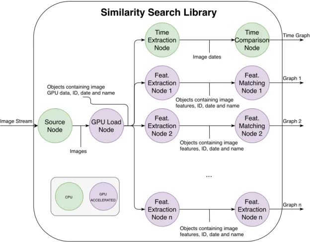
feature vectors), enabling future comparison. The feature matching section takes these image descriptors and uses them to compare images against each other, outputting a value (or score) which represents how similar the two images are. The final step con-structs or updates the image similarity graph, which can then be used for several types of queries. These steps and their implementations are further detailed in Chapter2and Chapter3. Most of the steps are parallelized and executed on the GPU, which maximizes performance.
As can be seen in Figure1.1, the key idea is to havemmachines execute feature ex-traction (using one or more algorithms), whilenother machines feed on that information in order to compute the graph, a process that is continuous and iterative. Typicallym < n
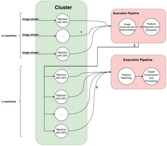
because, as we explained previously, the feature matching and graph construction step is more computationally expensive than the image processing and feature extraction steps. Taking a close look at Figure1.1, the firstmmachines process the stream (or streams), download the images and extract features from them (step 1). These machines can even extract features from multiple computer vision algorithms (which have different use cases,
further detailed in Chapter2). This saves time and resources, by keeping the image data in GPU memory and saving in CPU-GPU and GPU-CPU communication overheads. After the features are extracted, they are shared with the othernmachines (step 2), which then execute feature matching and compute the graph (step 3), outputting a graph (or several, depending on the amount of computer vision algorithms used) similar to what can be observed in Figure1.2.
Machine with GPU Machine with GPU Machine with GPU Machine with GPU Cluster Image stream Execution Pipeline Feature Detection and Extraction Feature Matching Graph Construction and Processing Execution Pipeline 1 2 3 Image download and preprocessing ... Machine with GPU ... Image stream Image stream m machines n machines
Figure 1.1: Distributed Pipeline
take advantage of the diversity of computer vision algorithms for different use cases. For
instance, some algorithms may be better at detecting objects in images, while others may be more suited towards detecting humans. Processing and making this data available all in one, parallel, execution instead of multiple executions (one for each algorithm) saves the user time, since the image is already downloaded, preprocessed and loaded on the GPU.
The querying process is identical to the one just described. A machine downloads the query image, pre-processes it and performs feature extraction. It then shares the image features with the machine (or machines) that contain the previously computed graphs. These machines, in turn, perform feature matching between the query image features and the previously computed features. They use this result in order to index the query image in the graph. Once this indexing process is complete, a graph primitive (such as Dijkstra’s algorithm) is executed, in order to compute the relevant query (e.g., find then
closest matches).
1 . 4 . CO N T R I B U T I O N S
query on the previously computed graph (or graphs). For instance, if we were to perform a query on the (tiny) graph present in Figure1.2, in order to obtain the most similar image to image 1, we would learn, through Dijkstra’s algorithm, that such an image is image 3 (considering that the lower the score, the more similar two images are). The usefulness of Dijkstra’s algorithm becomes more obvious with larger graphs, as they may contains hundreds of thousands of nodes and hundreds of millions of edges.
Figure 1.2: Example graph
To conclude, there are several different configurations that our solution can be
exe-cuted in (e.g. varyingmandn), each with different advantages. We may require more
diversity in our outputted graphs, or we may require sheer speed for a single computer vision algorithm. This means our library needs to be easily configurable and parametriz-able, in order to meet the user’s needs. Besides the different pipeline configurations, there
are also several different feature detection algorithms, graph construction and processing
libraries that can be used. The intent is to develop the library so that these components are easily interchangeable and, where they are not, we need to make sure that the ones used are the most efficient in order to achieve a better, faster solution.
1.4 Contributions
This thesis presents the following contributions:
• A solution that is able to process images and extract some number of features from them (using different algorithms for different features and use cases).
• A system that is able to take advantage of the graphs in order to process query images to determine images similar to them, both visually and in time.
• A system that outputs graphs that contain diverse information about all images processed, allows comparisons between them and enables users to take advantage of them for numerous use cases.
• A scalable system, capable of taking advantage of clusters vertically (by harnessing the power of each cluster node as much as possible) and horizontally (by harnessing the power of every single node), as well as take advantage of the power of GPU-accelerated algorithms.
• Several experimental evaluations detailing the performance of our solution with large image datasets.
1.5 Document Structure
In this chapter we introduced the problem this thesis attempts to tackle and the contri-butions it intends to make. We presented the motivation behind our work, the problems that it must face and their solutions.
In Chapter2, we introduce the architecture of the NVIDIA GPU and how it benefits our work, along with an introduction to GPU programming using CUDA. We also present the current state of the art for many different modules, libraries and algorithms our
solution intends to take advantage of such as feature detection, description and matching, graph construction and processing, and distributed computing. Chapter2 finishes off
with a comparison of modern libraries similar to the one we intend to build.
In Chapter3 we cover a top-level view of our system, its architecture and how it works.
Chapter4covers through the implemented solution thoroughly, entering into detail about every section and nuance of the system. Leaving these chapters, the reader should be able to understand the logic behind our choices and have an understanding of how to build such a system.
Chapter5details the experimental evaluations of our library, measuring its perfor-mance and precision.
Finally, Chapter6finishes off by extracting conclusions derived from our work, as
C
h
a
p
t
e
r
2
S t a t e o f t h e A rt
This Chapter presents the current state of the art in the areas this thesis covers. It starts by presenting the architecture of GPUs and their programming. It then covers several computer vision algorithms, how they work and their advantages and disadvantages. We also provide a preliminary benchmark for these algorithms, in order to compare them. We then cover feature matching techniques as well as GPU accelerated solutions for them. Afterwards, we detail and compare GPU graph processing libraries and distributed stream processing libraries. We finalize by presenting several image processing systems similar to our own.
2.1 GPU Architecture and Programming
Graphics Processing Unit (or GPU, for short) is a specialized, programmable electronic circuit designed for the rendering of images, animations, videos and everything related to computer graphics. It is optimized for the execution of vector transformations, matrix calculation and operations, and floating point operations. GPUs are frequently used in gaming systems, animation rendering and video processing, being highly efficient at
those tasks. They are good for and designed to process everything related with computer graphics. GPUs are in everyday systems, from personal computers to mobile phones and gaming consoles. These circuits have a highly parallel architecture, making them more efficient than many modern CPUs at the computation of certain, highly parallelizable,
algorithms.
financial sector and many more. Several industries now take advantage of the computa-tional power of GPUs, due to the fact that a GPU typically has thousands of cores while a CPU only has a few, as Figure2.1illustrates. GPUs have been designed, since their con-ception, for highly-parallel intensive tasks, which makes them perfect for certain types of computations, and many times faster than CPUs. In response to the emergence of the necessity of using GPUs for general purpose computation, some libraries, APIs and frame-works emerged that enable the programming of GPUs in a much simpler fashion, such as NVIDIA’s CUDA [25] (for NVIDIA graphics cards) and OpenCL [36] (which supports a broader range of GPU manufacturers including NVIDIA and AMD), which abstract the programmer from low-level GPU details.
Figure 2.1:CPU vs GPU cores1
2.1.1 NVIDIA Architecture
There are several NVIDIA graphics cards microarchitectures that were developed over time, however, we cover only the basics that are transversal to all modern microarchitec-tures and explain how they relate to the execution of parallel programs and algorithms, using as example the most modern NVIDIA microarchitecture named Pascal [34].
The architecture of a Pascal GPU can be observed in Figure2.2. It breaks down into several simpler components, of which we name a few:
• Graphics Processing Clusters, composed of 10 texture processing clusters (TPCs)
• Texture Processing Clusters, composed of 2 streaming multiprocessors (SMs)
• Streaming Multiprocessors
• Memory controllers
• PCIe host interface, to communicate with the host device
1Image taken from the NVIDIA website athttp://www.nvidia.com/object/what-is-gpu-computing.
2 . 1 . G P U A R C H I T E C T U R E A N D P R O G R A M M I N G
Figure 2.2: Pascal microarchitecture GPU, taken from [34].
NVIDIA GPUs process instruction streams in groups of 32 threads called warps. Each warp shares an instruction counter and every thread in the warp executes the same in-struction simultaneously. If threads within a warp take different execution paths (e.g.
in conditional statements), warp divergence occurs and performance is significantly re-duced. A group of 1 to 32 warps is called a thread block, and threads within a block have access to a piece of shared memory. Work is partitioned by assigning it to blocks and threads within blocks through thread and block IDs. Each block (occasionally, and in some architectures, more than one) is executed on one of the streaming multiprocessors (SM) of the GPU.
The architecture of the streaming multiprocessor (SM) can be observed in figure2.3. An SM consists of several cores (which perform arithmetic, logic and floating point oper-ations), special function units (SFUs, which execute special functions such as sin, cosine and square root), load/store units (LD/ST, which calculate source and destination ad-dresses), instruction buffers which contain instructions for the processing units, and
warp schedulers and dispatch units that issue instructions to warps. Finally, the SM has a 64KB shared memory and L1 cache, allowing threads within thread blocks to cooperate between them and cache data. The particular SM shown in figure2.3contains 64 cores and is part of the Pascal microarchitecture.
Figure 2.3: Pascal streaming multiprocessor, taken from [34].
in the Pascal microarchitecture) and have lower throughput and higher latency than any modern CPU core, they can execute many simple computations very quickly and achieve massive parallelism that can not be matched by any CPU on the market.
2.1.2 Programming: CUDA
Compute Unified Device Architecture (CUDA) is a parallel computing platform and programming model developed by NVIDIA for general purpose computing in graphics processing units. It enables programmers to significantly speed up computing applica-tions by offering them a platform that allows them to run programs developed in C, C++,
Fortran, and other languages, on the GPU. It removes the need to express computation through the programming of shaders as was needed before frameworks such as CUDA and OpenCL first emerged and has the great advantage of not having any overheads, as NVIDIA’s GPUs are developed to run CUDA code, and they excel at it. This makes CUDA-capable NVIDIA GPUs highly efficient at both the computation of graphics and
the general purpose computing tasks that we wish to execute.
2 . 1 . G P U A R C H I T E C T U R E A N D P R O G R A M M I N G
Section2.1.2) within a grid.
Typically only one kernel executes at a time, except in very modern GPUs, where spare resources are assigned to a second kernel whilst the first is running. Kernels can also execute in parallel, where blocks from several kernels are executed simultaneously in a grid. It is also possible to use certain ordering primitives in order to implement absolute ordering between kernels.
In sum, groups of threads (warps) are organized into thread blocks (which are exe-cuted on SMs) and blocks are organized into grids. The hierarchy of threads employed by CUDA can be observed in Figure 2.4. As can be seen, each single thread has a pri-vate local memory used for function calls and other functionalities usually related to the programming language being used. Threads are organized into blocks which have a per-block shared memory. This shared memory allows threads within blocks to cooperate, however, threads that belong to different blocks can not cooperate. This means we can
only achieve thread cooperation at the block level, and rarely at the whole program level. This is why it is best to run programs with low dependencies between calculations, as cooperation can be expensive in GPUs. Global memory (in the case of the NVIDIA Pascal Titan X, 12GB in size and with higher bandwidth than typical CPU memory) is used by the kernels running on grids (and blocks within grids) for communication and sharing computation results.
Figure 2.4:CUDA Thread Hierarchy2
The execution model is detailed in figure2.5. As we can see in this example, the host specifies two kernels to execute. The first kernel is assigned to Grid 1, which contains 6 blocks of threads while the second kernel is assigned to Grid 2. The vertical black arrow on the left represents time, meaning kernel 1 executes before kernel 2. Each block contains, in this example, 15 threads. Note that each block (or more, depending on shared memory usage per block) is executed on a streaming multiprocessor and each thread within a block is executed on a CUDA core within the SM (illustrated in figure
2.3). It is important to consider that these details are abstracted when writing CUDA code, and the programmer does not need to worry about such low level details unless he wants to fine-tune his code to be extremely efficient. Most of the time, a simple CUDA
implementation is sufficient for the objective of accelerating computation and achieving
much faster performance than would be achievable on a CPU.
2 . 2 . I M AG E F E AT U R E D E T E C T I O N A N D D E S C R I P T I O N O N G P U S
2.2 Image Feature Detection and Description on GPUs
There are several algorithms to detect visual features and describe images, with varying performance and precision. Some algorithms describe images in a more precise way, while others execute faster. Some are more adequate to detect human faces, while others excel at object detection. If we require very precise features and image descriptors, in order to avoid similar but different images to be detected as the same image, there are algorithms
that provide that. However, if we want our solution to have good performance, and do not mind loss of precision in the image feature vector, we must choose an algorithm that meets those requirements.
Since our objective is to build a graph capturing several image similarities and we intend to process very large amounts of images, precision can be relaxed to allow for faster extraction. In order to achieve even better performance, we consider the GPU-Accelerated versions of some of these algorithms.
The algorithms shown in this section are some of the most important algorithms that detect and extract features from images. An image feature vector consists of a vectorial representation of the image, allowing us to considerably reduce the image’s size and still be able to recognize and compare it with different images, which is useful when
considering the amount of images we need to process and store in memory. We only cover algorithms that are relevant to our work.
In the coming subsections, we briefly describe each algorithm and how it functions. We will process images using a selection of these algorithms in order to extract visual features. Later, using these, we will be able to compare images and calculate how similar they are.
2.2.1 OpenCV
Open Source Computer Vision (OpenCV) [3] is, an open-source computer vision and machine learning software library. It contains several algorithms for computer vision, from modelling 3D objects to detecting features from images. It has a very big community, number of contributors and number of users, making it a library with great support and number of features. Additionally, it contains high support for CUDA, enabling us to accelerate these algorithms’ executions on our GPU cluster, without the need to develop specialized CUDA kernels. Although the CUDA interface is still being developed as of the moment of writing this document, support for most of the algorithms we tested is widely available.
2.2.2 Histogram of Oriented Gradients
Histogram of Oriented Gradients (HOG) [8] uses, as the name suggests, a histogram of gradients to describe an image. It first computes the vertical and horizontal gradients of an image. Afterwards, the algorithm calculates the magnitude and direction for each gradient, where the direction points to the direction of the change in intensity and the magnitude points to how big the actual change is. Calculating gradients allows us to know the locations of the images where a sharp change in intensity occurs, therefore allowing us to identify the edges of the image, which are typically very useful for identifying visual signatures. An example of the gradients calculated from changes in intensity can be observed in Figure2.6.
Figure 2.6: HOG Visual Features3
After the gradients are calculated, the image is then divided in 8x8 cells, and a his-togram of gradients is calculated for each of the cells. The hishis-tograms have 9 bin values, each bin corresponding to an angle, as explained below.
The histogram is calculated and represented in an array where each index of the array corresponds to a bin of the histogram which, in turn, corresponds to the angle, in degrees, of the gradients in that cell. The value of each bin corresponds to the contribution of each gradients’ magnitude. An example histogram can be observed in Figure 2.7. The more value the histogram has in a certain bin, the higher the magnitude of the gradient is for that angle. The bins correspond to the angles 0, 20, 40, 60, 80, 100, 120, 140 and 160. It is important to note that if the angle is between 160 and 180, it contributes proportionally to the 0 and 160 degree bins [22].
The last step consists of calculating the final feature vector for the entire image. All the vectors (histograms) previously calculated are concatenated into one vector of 3780 dimensions. Afterwards, we are left with a histogram describing the image itself. It de-scribes the images’ changes in intensity by distributing them by the angle of the direction
3Taken from the scikit-image website athttp://scikit-image.org/docs/0.11.x/auto_examples/
2 . 2 . I M AG E F E AT U R E D E T E C T I O N A N D D E S C R I P T I O N O N G P U S
Figure 2.7:HOG Histogram
of the intensity.
This algorithm is typically used for human detection,i.e., face detection, pedestrian detection. It can also detect humans in different poses, from different angles. Due to
its precise ability to identify sharp edges in images, it is one of the better performing algorithms for that purpose.
2.2.3 Scale-Invariant Feature Transform
Key points represent locations of interest in an image. These are points that stand out and, when combined with each other, are able to describe the image visually. Key points are important for image description because they are usually unique, and enable diff
er-entiation between images. Image key points are associated with visual corners,i.e., the point where the directions of two edges change, meaning the gradient has a high variation. Several of these key points enable us to uniquely identify an image. Figure2.8shows us the key points for an example image. The size of the circle represents the size of the key point and the line within each circle represents its orientation.
A big problem that Scale-Invariant Feature Transform (SIFT) addresses is the fact that some algorithms are not scale-invariant. This means that a corner may not be a corner if the image is scaled. If we zoom into a corner enough, it may become flat and, thus, not be a corner any more (or atleast not be detected as one).
In order to address this, the authors in [20], developed SIFT. The algorithm works by extracting key points and computing their descriptors. SIFT first applies the scaling mechanism, which consists of scale-space filtering. The images are searched for local extrema,i.e., one pixel in the image is compared with several neighbours in higher and lower scales and, if it is a local extrema, it is a potential key point and is best represented
4Image taken from the OpenCV Documentation at https://docs.opencv.org/3.3.0/da/df5/
Figure 2.8: SIFT Key points4
in a certain scale. So, in sum, a pixel is tested for potential candidacy of being a key point in several different scales, thus achieving scale-invariance, as the name promises.
Once the potential key points are found, they are first filtered for noise and then assigned an orientation, in order to make the algorithm rotation-invariant (i.e.resistant to rotations of the image).
The key point descriptor is created for each key point, outputting a histogram of 128 bin values. Finally, this set of key point descriptors is what enables us to identify and compare the image.
The features extracted are both distinctive and precise, making this a robust algorithm, able to compare images correctly with high probability. The only issue with this algo-rithm is the fact that it is slower than most algoalgo-rithms, which is what the next algoalgo-rithm addresses.
2.2.4 Speeded-Up Robust Features
In order to address the performance issues in SIFT, the authors in [1] created a speeded-up version of the algorithm. They developed a new method for the scale-space filtering which, in short, has a different approximation for the Laplacian of Gaussian (used for scale-space
filtering in edge detection) than the one used in SIFT. It is not only a faster computation in itself, but it can also be computed in parallel. Additionally, it has several optimization parameters, such as bypassing the part of the algorithm that makes it rotation-invariant, since many applications do not require it.
2 . 2 . I M AG E F E AT U R E D E T E C T I O N A N D D E S C R I P T I O N O N G P U S
also an optimization, as fewer dimensions make the algorithm faster but the features less distinctive. However, it is a trade-offsome applications may want to make. Several other
optimizations are detailed in the paper, but the basis of SURF is a lot of improvements and parametrizations in each of the SIFT steps, resulting in an all-around faster algorithm, albeit less precise.
2.2.5 Features from Accelerated Segment Test
The motivation behind the Features from Accelerated Segment Test (FAST) algorithm [28] derive from the fact that feature detectors as the ones showed previously are not particularly fast enough for a real-time application.
This algorithm works by select a pixelp, to be tested as a key point candidate, and calculating its intensity Ip. Considering a threshold value t and a circle of 16 pixels
around pixelp, the algorithm considers pixelpto be a corner if there exists a set ofn(in the paper,n=12) contiguous pixels that are brighter thanIp+t or darker thanIp−t.
In order to speed up this test, the algorithm only examines four pixels (at opposite sites of the circle). If atleast three of these four points are brighter thanIp+t or darker
than Ip−t, then the pixel is considered a candidate to be a corner. After determining
potential candidates, the algorithm runs these computations again for all points of the circle for each candidate, in order to determine the final corner pixels.
Some issues (such as redundant features) arise from this methodology, however they are solved using a machine learning approach and non-maximum suppression, described in the paper.
It is important to note that this algorithm only detects key points, it does not compute descriptors. In order to compute a feature descriptor using this algorithm, we must use another algorithm in conjunction with FAST for the computation of the descriptor. The key points detected by FAST can be observed in Figure2.9.
Figure 2.9: FAST Keypoints
4Image taken from the OpenCV Documentation at https://docs.opencv.org/3.0-beta/doc/py_
In sum, this algorithm is significantly faster than the others described in regards to the key point computation, but it is not as precise and may suffer from images with a lot
of noise. Also, it is still dependant on another algorithm in order to compute a feature descriptor, as it is only a key point detector.
2.2.6 Vector of Locally Aggregated Descriptors
The vector of Locally Aggregated Descriptors (VLAD) [18] algorithm consists of, as the name suggests, aggregating local descriptors in a vector. The main focus of the develop-ment of this algorithm was on three constraints: search accuracy, efficiency and memory
usage.
The algorithm first computes a set ofkvisual words C={C1, ..., Ck} (i.e.,
neighbour-hoods or small parts of the image where features are extracted from) using k-means. Then, each local descriptor xis associated with its nearest visual word and the difference
be-tween the local descriptor and the associated visual word is computed. This difference
characterizes the distribution of the vector with respect to the center. The vector is then computed as the sum of all the differences between the local descriptor and the associated
visual word for each of thekneighbours.
This vector then serves as input in order to compute a code of B bits, encoding the image. Several optimizations are performed in order to produce this encoding (such as dimensionality reduction and indexation), better described in the original paper.
This algorithm is very accurate and fast in searching operations, being able to search a 10 million image dataset in only 50ms, achieving its design goals of memory usage, search accuracy and efficiency.
2.2.7 Deep Learning Visual Features
The algorithm developed by the Visual Geometry Group (VGG) [31] relies on a convolu-tional neural network, trained to classify images. Using their algorithm and a pre-trained network containing millions of images, we can extract visual features from images. The algorithm outputs a 4096 dimensional feature vector, containing the neural network activations.
As this algorithm relies on an external neural network, it is only as good as the network itself, and is dependant on the images that it was trained with. Also, the activations are normalized, enabling us to use the feature vectors as as generic features for image similarity calculation.
2.2.8 Binary Robust Independent Elementary Features
2 . 2 . I M AG E F E AT U R E D E T E C T I O N A N D D E S C R I P T I O N O N G P U S
of single-precision floating point numbers) which means each SIFT descriptor occupies around 512 bytes in memory. This does not seem like much, but we if consider processing 10 million images, for example, it amounts to more than 5GB. This is a very large amount to hold in memory and becomes a big constraint in programs that wish to process and match large amounts of images.
BRIEF takes advantage of the fact that not all dimensions of a feature descriptor are needed to perform feature matching. It is possible to compress these descriptors, using methods like locality sensitive hashing. These compression methods convert descriptors from floating point numbers into binary strings. In order to compare such binary strings, for feature matching, it is possible to use a norm such as Hamming distance. BRIEF uses a unique way (which is detailed in the paper) to find binary strings directly, without the need to find descriptors first. This means the memory issue is addressed directly, as we do not require computing a feature descriptor first and only then compress it.
It is important to note that BRIEF is only a feature descriptor. It does not detect key points. In order to use BRIEF, we have to pair it with another algorithm that can perform feature detection (such as SIFT, SURF or FAST, for instance).
This algorithm is a fast and light feature descriptor, while also providing good preci-sion when matching. It is suitable for libraries that intend to process large amounts of images and are constrained by memory.
2.2.9 Oriented FAST and Rotated BRIEF
Oriented FAST and Rotated BRIEF (ORB) [29] is an algorithm that, essentially, consists of a fusion between the FAST key point detector (previously detailed in Subsection2.2.5) and the BRIEF descriptor (Subsection2.2.8). This is, however, not a simple concatenation of these algorithms, as it employs several strategies to improve precision. First of which is tweaking the key point detection so that it is rotation invariant (as FAST does not provide this natively). Additionally, it improves the precision of BRIEF descriptors by tweaking them to better define the orientation of the key points.
This algorithm takes the best of the FAST detector and BRIEF descriptor and attempts to solve or lessen the impact of their downsides. ORB is much less memory intensive than algorithms such as SURF and SIFT and provides a much faster matching solution, although precision is not nearly as good as in these algorithms.
2.2.10 Preliminary Benchmark
In order to properly compare the performance of the above algorithms, we created a simple testbed that enabled us to benchmark and test the algorithms. We only considered algorithms supported by OpenCV, as they are easier to implement, well established, and support for them is widely available. It also enables us to easily switch between different
Table 2.1: OpenCV Feature Detection and Description Algorithm Comparison
Algorithm Feature Extraction GPU (ms/image)
Feature Extraction CPU (ms/image)
SURF 16.3 41.3
HOG 5.2 19.9
ORB 34.8 48.8
of 500 images from the YFCC100M dataset [35], measuring the average time it took to detect and describe the features from each of those images, for each algorithm. We do not consider the download time for the images or the GPU upload time in this test, in order to focus more on the execution of the algorithm itself and due to the fact that these overheads are inevitable and do not depend on any algorithm. The results displayed are an average of three executions. Results for the algorithms executed on the CPU are also displayed. These are aggregated in table2.1. The algorithm represents both the feature detector and descriptor, and the times displayed consist of the time it takes to detect key points in an image and generate a feature vector to describe the image. As previously explained, this vector is the vectorial description of an image and enables us to compare images with each other.
The testbed consists of an Asus N751JX laptop, with an Intel Core i7 4720HQ Proces-sor with a clock speed of 2.6GHz (turbo boost up to 3.6GHz) and a NVIDIA GeForce GTX 950M with 2GB of VRAM.
As we can observe from the table, it is clear that running these algorithms on a GPU incurs in a significant speedup over execution on the CPU. In all three algorithms that we tested, the benefit of using the GPU is clear. Obviously, any small microsecond gain is very significant in libraries that intend to process millions of images. Out of these three, HOG executes faster, although its feature matching process is typically slower, and its features are much more memory intensive than the other algorithms tested. The ORB algorithm has a much higher extraction time than its peers, which is expected, as its memory saving techniques incur in a higher processing time. In this case, we are trading off processing time for less memory usage, while in other cases (such as the
HOG algorithm) we benefit from speed while sacrificing memory usage. SURF is a more balanced algorithm. Although it is less precise than HOG, its features are less memory intensive. It is important to note that each of these algorithms excel at different tasks and
have different use cases. For instance, and as described in the previous subsections, HOG
is more adequate for human and face detection, while SURF and ORB are algorithms more suited towards object detection.
2 . 3 . F E AT U R E M ATC H I N G
In conclusion, in order to meet speed requirements, for instance, one may use the HOG algorithm. However, if memory is an issue, it may be wise to use an algorithm such as ORB, or even SURF to meet a balance between both. Nonetheless, usage of OpenCV entails in a great advantage: the ease of interchangeability of algorithms on the fly enables great adaptability to different constraints.
2.3 Feature Matching
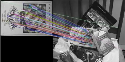
Feature matching is an essential part of our work, as it is necessary to be able to compare images between each other and calculate how similar they are. It is also a necessity for us to query the system with an image and be able to tell if that or a similar image exists. Being able to tell if two images are the same or, at least, similar is very useful, as we went over in Chapter 1. Also, the ability to detect if a certain object is in a certain picture (e.g. a human face among a picture of a crowd of people) is a very useful feature with many use cases. This is the functionality provided by feature matching. After computing the feature descriptors of images, we need to run a matching algorithm between them, outputting matches between images.
2.3.1 k-Nearest Neighbours
k-Nearest Neighbours is a machine learning algorithm used for classification and re-gression. The algorithm consists of a training phase, where it is fed examples of multidi-mensional features, each with a class label. Afterwards, in the classification phase, the algorithm classifies an unlabelled feature vector by assigning it the label that is most fre-quent among its k-nearest neighbours. There are several metrics to compute the k-nearest neighbours, the most common being Euclidean distance. It is a very simple and powerful algorithm.
The author of SIFT proposed in [21] a ratio test to evaluate the similarity of two images. It is necessary in order to discard features that are not useful and possible false matches, such as ones generated from background clutter in the image. It takes the ratio between the distance of the closest match and the distance of the second-closest match (usually paired with k-NN, withk= 2). This discards false matches well because there is usually a number of other false matches within similar distances, due to the high dimensionality of features. In the paper, the author shows that by rejecting matches with a ratio greater than 0.8 we can eliminate 90% of the false matches while only discarding less than 5% of correct matches. Applying this test to the matches obtained by k-NN across all features of the query image, we are left with the matches between two images and we can tell with a good degree of confidence whether or not the images are similar. We can also compute how similar they are by designing a score that measures the ratio between good matches (the ones filtered by the ratio test) and the total number of matches (before the filtering), and even if they contain the same objects.
Figure 2.10: k-NN Illustration
k-NN Illustration with k = 3. The red cross is the point being tested, while the blue dots are the points from the training data.
Figure 2.11:Brute-force matching with k-NN
2 . 3 . F E AT U R E M ATC H I N G
Note that features of images are usually corners in most algorithms, as explained in section2.2. We can see this matching in action in figure2.11, taken from the OpenCV [3] website. The algorithm picks a feature from the query image (left) and executes k-NN as described above, comparing it with the features from the training image (right). It selects the two closest features (k= 2) and performs the ratio test, in order to filter out most incorrect matches. It does this for all features of the query image, finding all matches. Each line is a match,i.e., it is drawn between the two features of both images that more closely match. As we can see, brute-force matching with k-NN finds a lot of matches between the two images (albeit still containing some noise) and can correctly assume their similarity. In this case, the algorithm is finds an object (the box on the query image on the left) in an image with a group of objects (the training image on the right).
2.3.2 GPU-Accelerated k-Nearest Neighbours
Following the line of thought we have been following so far, we want to accelerate our solution wherever we can and feature matching is a computationally intensive step. Obvi-ously, this also means using a GPU-Accelerated implementation of k-Nearest Neighbours, as it is a highly parallelizable algorithm, which means it can be significantly sped up by doing so.
OpenCV features a CUDA implementation of the brute-force k-nearest neighbours matching algorithm, which significantly speeds up the computation. It is easy to use, like most CUDA libraries in OpenCV, and it can be easily interchanged with the CPU version, if there is need to do so. There is also a lot of recent work on the topic of executing k-NN on GPUs.
The approach in [11], implemented using CUDA, works by specifying two CUDA kernels where the first calculates the distance matrix between the query points and the training points, and the second sorts the distance matrix, retrieving thekpoints closest to the query point. The big optimization is in reformulating the way the distance matrix is calculated by optimizing the distance calculation using linear algebra and computing it using the CUBLAS library (CUDA implementation of the highly optimized BLAS linear algebra library). The experiments run by the authors of that work show that the CUBLAS implementation is up to 62X faster on SIFT feature matching than the Approximate Nearest Neighbour (ANN) C++ library.
Gieseke et al. [12] combine k-dimensional trees and GPUs by proposing a variant of k-d trees called buffer k-d tree, showing good speedup against other k-d tree GPU
implementations and brute-force k-NN.
The work in [26] attempts to reduce the search space by partitioning datasets into several groups in order to cluster similar items and using locality-sensitive hashing (LSH) to speed up the query process. The GPU implementation shows a 40X speedup over other LSH single-core CPU approaches.
redundant distance computation (i.e., reducing the search space) and executing massively-parallel computation on the GPU. It strives to achieve balance between minimizing redundancy and preserving regularity (which means better performance on GPUs and linear algebra libraries). Sweet k-NN is a very recent approach and shows up to 44X speedup over the work in [11] in some datasets. As far as we are aware, this is the current state of the art in the area of GPU-accelerated k-nearest neighbours algorithms.
The key points that are important to our work is the ability to store the feature descrip-tors correctly in GPU memory in order to efficiently perform comparisons and reducing
the search space, in order to perform less redundant computation and result in overall lower execution time, while maintaining precision. The OpenCV implementation is easy to use and to integrate with our work, since features will already be extracted using OpenCV. It is the simplest solution, while also having GPU support. We also consider using Sweet k-NN in the future, supporting the modularity design goal of our solution, and being able to easily change between implementations.
2.4 GPU Graph Processing
In the context of our work, after image features are computed, we need to organize them in a graph. Each node in the graph corresponds to an image (its features) and the edges between nodes correspond to the similarity between them. A node hasnedges for each of itsnneighbours,i.e., itsnmost similar images. The construction of this graph is a challenge due to its size, the actual computation, the memory constraints (how to store the graph in multiple GPUs and multiple machines) and, most importantly, the necessity of executing queries efficiently and quickly on the computed graph.
After the computation, the output is a graph as big as the number of images processed and containing as many edges as there are similar images, meaning a very large dataset will output a very large graph. This graph is key to our design goal of being able to query images for their similarity, and the way to achieve that is through running primitives on the graph that allow us to extract information from it.
Once again, we turn to GPUs in order to solve all of these challenges, from graph con-struction to the execution of primitives (such as breadth-first search) on the constructed graph. Like in the case of image feature detection and description detailed in Section2.2, graph processing benefits greatly from the parallelism offered by GPUs. There are
sev-eral libraries that support high-performance graph processing on the GPU and we will examine the state of the art solutions in this section and explain which fits our work better.
2.4.1 Solutions
2 . 4 . G P U G R A P H P R O C E S S I N G
subsequently:
Single-node CPU Systems These types of systems are the most common (and only in the last few years have we begun to see a lot of research on the topic of GPU graph processing). There are several solutions in this category. From hard-wired im-plementations of graph primitives to several frameworks like Ligra [30], that ab-stract the programmer from low-level parallelism details, and allow focus on the development of the actual graph primitives. These solutions can take advantage of multi-core architectures and can achieve good performance, however, they are still significantly slower than recent GPU implementations.
Distributed CPU Systems These systems take advantage of several machines with sev-eral CPUs, splitting graph computations between them. There is an obvious advan-tage of scaling the solution to multiple machines and CPUs, however, these types of solutions incur in a high communication cost in order to synchronize information between the different machines and a high monetary cost of acquiring the hardware
or renting a cloud infrastructure.
Low-level GPU Implementations These implementations are the best of all the cate-gories. Taking advantage of the GPU’s massive parallelism for graph processing allows for very fast solutions, when compared to the other categories. The big disadvantage of this solution is the challenge involved in programming GPUs.
High-level GPU Frameworks These systems are typically slower than low-level GPU im-plementations, due to the overheads inherent to high-level programming libraries and the lack of graph primitive optimizations that can be achieved when program-ming low-level solutions. However, the great advantage of this category of solutions is the fact that the programmer is abstracted from the complicated, low-level details of GPU programming and can focus on the actual development of the primitive. Additionally, the overheads of using a framework are usually negligible when con-sidering the advantages.
Considering the focus of this thesis is not in the development and improvement of graph primitives or graph processing libraries, we chose to use a solution that falls in the High-level GPU frameworks category. Like stated in the beginning of this section, using GPUs to accelerate our overall solution is one of our design goals. Thus, we can benefit greatly from using a framework that allows us to focus on the actual implementation of the graph primitives we require (or even use a library that already has it implemented) and still take advantage of the massive speed-up offered by computing these primitives

![Figure 2.2: Pascal microarchitecture GPU, taken from [34].](https://thumb-eu.123doks.com/thumbv2/123dok_br/16525015.735967/31.892.131.824.151.557/figure-pascal-microarchitecture-gpu-taken-from.webp)
![Figure 2.3: Pascal streaming multiprocessor, taken from [34].](https://thumb-eu.123doks.com/thumbv2/123dok_br/16525015.735967/32.892.130.802.151.635/figure-pascal-streaming-multiprocessor-taken-from.webp)