Ana Carolina Costa Amorim
Bachelor of ScienceDevelopment of a Osirix plug-in for non-gaussian
diffusion MRI data: application to Breast.
Dissertation submitted in partial fulfillment of the requirements for the degree of
Master of Science in Biomedical Engineering
Adviser: Hugo Alexandre Ferreira, Assistant Professor, Faculty of Sciences of the University of Lisbon
Co-adviser: Rita G. Nunes, Assistant Investigator, Faculty of Sci-ences of the University of Lisbon
Examination Committee
Chairperson: Assistant Professor Carla Quintão Raporteurs: Adjunt Professor Margarida Ribeiro
Development of a Osirix plug-in for non-gaussian diffusion MRI data:
appli-cation to Breast.
Copyright © Ana Carolina Costa Amorim, Faculty of Sciences and Technology, NOVA University of Lisbon.
The Faculty of Sciences and Technology and the NOVA University of Lisbon have the right, perpetual and without geographical boundaries, to file and publish this dissertation through printed copies reproduced on paper or on digital form, or by any other means known or that may be invented, and to disseminate through scientific repositories and admit its copying and distribution for non-commercial, educational or research purposes, as long as credit is given to the author and editor.
This document was created using the (pdf)LATEX processor, based in the “unlthesis” template[1], developed at the Dep. Informática of FCT-NOVA [2].
A c k n o w l e d g e m e n t s
First and foremost, I would like to express my greatest gratitude to my adviser and co-adviser, Prof. Hugo Ferreira and Prof. Rita G. Nunes. Thank you for having the patience and listening to all of my doubts, questions and struggles. Thank you so much for giving me the opportunity to work with you, I truly enjoyed it!
Secondly, I would also like to give a big thank you to Filipa Borlinhas and Luísa Nogueira, who gave me images to work with and also valuable tips and information.
Thank you also to everyone in IBEB who helped me throughout these months. I really enjoyed the companionship, the amazing team work spirit, the long lunches and, in the last weeks, dinners and the elucidating discussions on how to write a thesis. It really motivated me to keep coming back to IBEB and work.
On a more personal note, I would like to thank everyone who helped me through all of these years. A big thank you to Patricia Paulino, who even though I only met two years ago, helped me so much and is someone I can call a good friend. I would also like to thank everyone who lived with me and had to deal with me, specially to my best friends Raquel Martins and Marina Teixeira. And of course, I want to give a shoutout to my second family, Mario, Ramalho, Miguel, Boiça, JR, Barreto and Vasco.
There is also an association that I have been a part of called BEST to which I would like to say a big thank you. Every single person in it is amazing and even though I have only been there for one year, I will miss it deeply.
A b s t r a c t
Breast cancer is the second leading cause of death by cancer and is the second type of cancer that is the most common among women, causing the death of 1500 women, every year, in Portugal. Over the past decades, with the improvement of imaging techniques and therapeutics, breast cancer mortality rate has been decreasing substantially. One of the imaging techniques used is diffusion-weighted imaging (DWI), which is the magnetic
resonance imaging method that is the most sensitive in detecting invasive breast cancer. There are several extensions of this technique that can be based on the premise that the environment is not homogeneous (non-Gaussian models).
The non-Gaussian models, take into account the presence of barriers and compart-ments that restrict the water molecules movement in the biological tissues, allowing the distinction between malignant and benign lesions in DWI. Taking into account that diffusion-weighted imaging is a non invasive method, the diagnosis through the
applica-tion of these models can become an alternative to biopsy.
The main goal of this dissertation was the development of a OsiriX plug-in that performs the non-Gaussian diffusion analysis of DWI in magnetic resonance imaging
data. Five non-Gaussian diffusion models were implemented in the application: diff
u-sion kurtosis imaging, intravoxel incoherent motion, gamma distribution, truncated and stretched-exponential. Parametric maps and region-of interest (ROI) parametric values were obtained for each model. In order to fit the various non-Gaussian diffusion
mod-els, the Levenberg-Marquardt algorithm was used. This algorithm finds coefficients x to
best fit the nonlinear function to the data. The x coefficients results in parametric maps
that are able to identify the tumour and also distinguish between malignant and benign lesions provided a comparison with the literature. During the application development, these functionalities were also used to study the dependence of fitted parameters on the number of b-values used and on the image noise.
An interface was developed with Objective-C on Xcode for OsiriX where the user gets to choose from five diffusion models in order to obtain parameric maps or values. It also
informs on the goodness of fit and it provides fitting plots of the data. The references of the models and extra information are also available in an help button.
Keywords: Diffusion Kurtosis Imaging, Intravoxel Incoherent Motion, Gamma
R e s u m o
O cancro da mama é a segunda causa de morte por cancro e é o segundo tipo de cancro mais comum entre as mulheres, matando todos os anos 1500 mulheres só em Portugal. Nos últimos anos, com a melhoria das técnicas de imagem e terapêutica, a taxa de mortalidade do cancro da mama tem diminuido substancialmente. Uma das técnicas de imagem usadas é a imagem ponderada em difusão (DWI), que é o método da imagem por ressonância magnética mais sensível na detecção de cancro da mama invasivo. Existem várias extensões desta técnica que se baseiam na premissa que o ambiente não é homogéneo (modelos não-Gaussianos).
Os modelos não-Gaussianos, têm em conta a presença de barreiras e compartimentos que restringem o movimento das moléculas de água nos tecidos biológicos, permitindo assim a distinção entre lesões malignas e benignas numa imagem ponderada em difusão. Sendo a imagem ponderada em difusão um método não invasivo de imagem por resso-nância magnética, o diagnóstico através da aplicação destes modelos pode se tornar uma alternativa à biópsia.
O principal objectivo desta dissertação foi o desenvolvimento de umplug-inpara o OsiriX que efectue a análise da difusão não-Gaussiana em dados de imagens de resso-nância magnética. Foram implementados cinco modelos de difusão não-Gaussianos na aplicação: imagem por curtose de difusão, movimento incoerente intravoxel, distribuição gama, truncado e “stretched-exponential”. Foram obtidos mapas paramétricos e valores paramétricos correspondentes à região de interesse (ROI). De forma a fazer o ajuste dos vários modelos de difusão não Gaussianos, foi aplicado o algoritmo Levenberg-Marquardt. Este algoritmo procura coeficientes de x de forma a fazer o melhor ajuste da função não linear aos dados. Os coeficientes de x resultam em mapas paramétricos que conseguem identificar o tumor e também distinguir lesões mailgnas de benignas, fornecendo compa-ração com a literatura. Durante o desenvolvimento da aplicação, estas funcionalidades foram testadas de forma a estudar a dependência dos parâmetros ajustados aos valores debusados e relação sinal-ruído.
Em conclusão, oplug-inpermite a visualização do tumor e a distinção entre lesões malignas e benignas.
C o n t e n t s
List of Figures xv
List of Tables xxi
List of Symbols xxiii
Acronyms xxv
1 Introduction 1
1.1 Context and motivation . . . 1
1.2 Objectives . . . 2
1.3 Dissertation plan . . . 2
1.4 Dissertation outputs . . . 3
2 Theoretic Underpinnings 5 2.1 Breast anatomy . . . 5
2.1.1 Benign vs Malignant lesions . . . 6
2.2 MRI . . . 6
2.2.1 Diffusion and MRI . . . . 7
2.2.2 Diffusion . . . . 9
2.2.3 Diffusion Weighted Imaging . . . . 9
2.3 Non-Gaussian Models . . . 11
2.3.1 Diffusion Kurtosis Imaging . . . . 11
2.3.2 Intravoxel Incoherent Motion . . . 13
2.4 Statistical distribution models . . . 15
2.4.1 Gamma Distribution . . . 15
2.4.2 Truncated Gaussian Distribution . . . 16
2.4.3 Stretched-Exponential Model . . . 16
2.5 State-of-the-art . . . 17
2.5.1 State-of-the-art of Diffusion Kurtosis Imaging . . . . 17
2.5.2 State-of-the-art of Intravoxel Incoherent Motion . . . 18
2.5.3 State-of-the-art of Gamma Distribution . . . 21
2.5.5 State-of-the-art of Stretched-Exponential . . . 25
3 Materials and Methods 27 3.1 Dataset and Acquisitions . . . 27
3.2 Image Processing Tools . . . 28
3.2.1 Producing parametric maps . . . 28
3.2.2 Obtaining parametric values with a ROI . . . 31
3.3 Testing the plug-in in images with differentb-values and noise . . . . 32
3.3.1 Differentbvalues . . . . 32
3.3.2 Different amount of noise . . . . 34
4 Results and Discussion 35 4.1 Parametric maps . . . 35
4.1.1 Interface . . . 35
4.1.2 DKI parametric maps . . . 38
4.1.3 IVIM parametric maps . . . 42
4.1.4 Gamma parametric maps . . . 45
4.1.5 Truncated parametric maps . . . 52
4.1.6 Stretched parametric maps . . . 54
4.1.7 Goodness-of-fit maps . . . 57
4.2 Parametric values obtained through ROIs . . . 59
4.2.1 Interface to obtain the parametric values . . . 59
4.2.2 Obtained parametric values . . . 60
4.3 Number ofbvalues and noise tests . . . 73
4.3.1 bvalues test . . . 73
4.3.2 Noise tests . . . 88
5 Conclusions and Future Work 101 Bibliography 103 A Testingbvalues and noise 109 A.0.3 Goodness of fit maps for the first combination ofbvalues removal 109 A.0.4 Goodness of fit maps of the maps with the noise added . . . 110
L i s t o f F i g u r e s
2.1 Anatomy of the breast. . . 6 2.2 Application of a radiofrequency pulse causing spins to align with the higher
energy state. . . 8 2.3 Pulse sequence diagram of a spin eco sequence. . . 10 2.4 Examples of images obtained with Diffusion Weighted Imaging (DWI). . . . 11
2.5 Probability distributions with the variation of kurtosis values. . . 12 2.6 Plot of signal attenuation of a well-perfused tissue with increasingbvalues. 14 2.7 Gamma distribution of five curves. . . 15 2.8 Parametric maps of a patient with malignant carcinoma. . . 18 2.9 Parametric maps of a patient with fibroadenoma. . . 19 2.10 Box plot distribution of the parameters by lesion type ofADC(a) parameter
using the mono-exponental model, andMD(b) andMK(c) parameters using the kurtosis model. . . 20 2.11 Box plots in breast lesions and normal tissue ofD(a),f (b),D∗(c) andADC
(d). . . 21 2.12 Parametric maps (D,f,D∗andADC) of a 25-year-old woman with a
fibroade-noma(thin arrow) and a simple cyst in her left breast. . . 22 2.13 Parametric maps (D,f,D∗andADC) of a 30-year-old woman with invasive
ductal carcinoma. . . 23 2.14 Evaluation of two fractional areas corresponding to frac < 1 and frac > 3 that
are considered to reflect the small cell component and perfusion, respectively. 24 2.15 a) Scatter plot of frac>3 vs frac<1; b) Scatter plot ofθvsκ; for the cancer and
not cancer group. . . 24
4.1 Interface of the plug-in. . . 36 4.2 Warning that appears when the user presses the "OK" button, next to the
parametric maps check boxes, and doesn’t select which model to run. . . 36 4.3 Warning that appears when the user trys to run the models on a parametric
map and not a DWI image. . . 37 4.4 Window that alerts the user to wait while the program is running. . . 37 4.5 Window that informs the user on the amount that was multiplied to which
4.6 Window that alerts the user that the process to produce parametric maps is
complete. . . 38
4.7 Images of a breast with malignant tumor (invasive ductal carcinoma): a) DWI image with thebvalue 50 s/mm2; b) DWI image with the Wiener filter applied. 39 4.8 MDparametric maps with an arrow indicating a malignant lesion. . . 40
4.9 MKparametric maps with an arrow indicating a malignant lesion. . . 40
4.10 MDparametric maps with an arrow indicating a benign lesion. . . 41
4.11 MKparametric maps with an arrow indicating a benign lesion. . . 41
4.12 D∗parametric maps with an arrow indicating a malignant lesion. . . 42
4.13 Dparametric maps with an arrow indicating a malignant lesion . . . 43
4.14 f parametric maps that show higher values of perfusion around the tumor area. 43 4.15 D∗parametric maps with an arrow indicating a benign lesion. . . 44
4.16 Dparametric maps with an arrow indicating a benign lesion. . . 44
4.17 f parametric maps that show high diffusion near the tumor area. . . . 45
4.18 θparametric maps with an arrow indicating a malignant lesion. . . 46
4.19 κparametric maps with an arrow indicating a malignant lesion. . . 46
4.20 S1 parametric maps with an arrow indicating a malignant lesion. . . 47
4.21 S2 parametric maps with an arrow indicating a malignant lesion. . . 47
4.22 S3 parametric maps with an arrow indicating a malignant lesion. . . 48
4.23 θparametric maps with an arrow indicating a benign lesion. . . 49
4.24 κparametric maps with an arrow indicating a benign lesion. . . 49
4.25 S1 parametric maps with an arrow indicating a benign lesion. . . 50
4.26 S2 parametric maps with an arrow indicating a benign lesion. . . 50
4.27 S3 parametric maps with an arrow indicating a benign lesion. . . 51
4.28 σ parametric maps with an arrow indicating a malignant lesion. . . 52
4.29 ADCparametric maps with an arrow indicating a malignant lesion. . . 53
4.30 σ parametric maps with an arrow indicating a benign lesion. . . 53
4.31 ADCparametric maps with an arrow indicating a benign lesion. . . 54
4.32 DDCparametric maps with an arrow indicating a malignant lesion. . . 55
4.33 αparametric maps with an arrow indicating a malignant lesion. . . 55
4.34 DDCparametric maps with an arrow indicating a benign lesion. . . 56
4.35 αparametric maps with an arrow indicating a benign lesion. . . 56
4.36 Goodness-of-fit maps for Diffusion Kurtosis Imaging (DKI), Gamma, Trun-cated and Stretched models applied to a breast with a malignant lesion. . . . 57
4.37 Goodness-of-fit map for DKI, Gamma, Truncated and Stretched models ap-plied to a breast with a benign lesion. . . 58
4.38 Goodness-of-fit maps for the Intravoxel Incoherent Motion (IVIM) models applied to a breast with a malignant lesion. . . 58
L i s t o f F i g u r e s
4.40 Alert that warns the user that the program can only run if on the displayed window is the image where the user draws the ROI. . . 60 4.41 Warning that alerts the user that the process to obtain the parametric values
is done running. . . 60 4.42 Warning that appears when the user is trying to save the results obtained but
without running a model first. . . 61 4.43 Results for the parametric values obtained through ROIS around the
malig-nant tumor (invasive ductal carcinoma) area. . . 61 4.44 Results for the parametric values obtained through ROIS around the benign
tumor (fibroadenoma) area. . . 62 4.45 Fitting plot for the DKI model of a DWI image of the breast with a malignant
lesion. . . 63 4.46 Fitting plot for the DKI model of a DWI image of the breast with a benign
lesion. . . 64 4.47 Fitting plot for the IVIM model of a DWI image of the breast with a malignant
lesion. . . 65 4.48 Fitting plot for the IVIM model of a DWI image of the breast with a benign
lesion. . . 66 4.49 Fitting plot for the Gamma model of a DWI image of the breast with a
malig-nant lesion. . . 67 4.50 Fitting plot for the Gamma model of a DWI image of the breast with a benign
lesion. . . 68 4.51 Fitting plot for the Truncated model of a DWI image of the breast with a
malignant lesion. . . 69 4.52 Fitting plot for the Truncated model of a DWI image of the breast with a benign
lesion. . . 70 4.53 Fitting plot for the Stretched model of a DWI image of the breast with a
ma-lignant lesion. . . 71 4.54 Fitting plot for the Stretched model of a DWI image of the breast with a benign
lesion. . . 72 4.55 MDmaps of a breast with a malignant lesion which show the quality decrease
when are applied with images with lessbvalues. . . 73 4.56 MKmaps of a breast with a malignant lesion which show the quality decrease
when are applied with images with lessbvalues. . . 74 4.57 D∗maps of a breast with a malignant lesion which show the quality increase
when are applied with images with lessbvalues. . . 75 4.58 Dmaps of a breast with a malignant lesion which show the quality decrease
when are applied with images with lessbvalues. . . 76 4.59 f maps of a breast with a malignant lesion which show the quality increase
4.60 θmaps of a breast with a malignant lesion which show the quality decrease when are applied with images with lessbvalues. . . 78 4.61 κ maps of a breast with a malignant lesion which show the quality decrease
when are applied with images with lessbvalues. . . 79 4.62 S1 maps of a breast with a malignant lesion which show the quality decrease
when are applied with images with lessbvalues. . . 80 4.63 S2 maps of a breast with a malignant lesion which show the quality decrease
when are applied with images with lessbvalues. . . 81 4.64 S3 maps of a breast with a malignant lesion which show the quality decrease
when are applied with images with lessbvalues. . . 82 4.65 σ maps of a breast with a malignant lesion which show the quality decrease
when are applied with images with lessbvalues. . . 83 4.66 ADCmaps of a breast with a malignant lesion which show the quality decrease
when are applied with images with lessbvalues. . . 84 4.67 DDCmaps of a breast with a malignant lesion which show the quality decrease
when are applied with images with lessbvalues. . . 85 4.68 α maps of a breast with a malignant lesion which show the quality decrease
when are applied with images with lessbvalues. . . 86 4.69 Goodness-of-fit map for DKI, Gamma, Truncated and Stretched models
ap-plied to a breast with a malignant lesion when the image with thebvalue 1000 s/mm2was removed. . . 87 4.70 MDmaps (scalling factor of 1×10⁶and in mm2/s) of a breast with a malignant
lesion (invasive ductal carcinoma) which show the quality decrease when are applied to images with 10%, 15%, 20%, 25%, 30% and 35% amount of noise, respectively.. . . 89 4.71 MKmaps (scalling factor of 1×10³with no units since it is dimensionless) of
a breast with a malignant lesion (invasive ductal carcinoma) which show the quality decrease when are applied to images with 10%, 15%, 20%, 25%, 30% and 35% amount of noise, respectively. . . 90 4.72 D∗maps (scalling factor of 1×10⁶and in mm2/s) of a breast with a malignant
lesion (invasive ductal carcinoma) which show the quality increase when are applied to images with 10%, 15%, 20%, 25%, 30% and 35% amount of noise, respectively. . . 91 4.73 Dmaps (scalling factor of 1×10⁶and in mm2/s) of a breast with a malignant
lesion (invasive ductal carcinoma) which show the quality decrease when are applied to images with 10%, 15%, 20%, 25%, 30% and 35% amount of noise, respectively. . . 92 4.74 f maps (scalling factor of 1×10⁴ and in %) of a breast with a malignant
L i s t o f F i g u r e s
4.75 θmaps (scalling factor of 1×10⁴and in mm2/s) of a breast with a malignant lesion (invasive ductal carcinoma) which show the quality increase when ap-plied to images with 10%, 15%, 20%, 25%, 30% and 35% amount of noise, respectively. . . 94 4.76 κ maps (scalling factor of 10 and with no units since it is dimensionless) of
a breast with a malignant lesion (invasive ductal carcinoma) which show the quality increase when applied to images with 10%, 15%, 20%, 25%, 30% and 35% amount of noise, respectively. . . 95 4.77 S1 maps (scalling factor of 1×10³ and in %) of a breast with a malignant
lesion (invasive ductal carcinoma) which show the quality decrease when are applied to images with 10%, 15%, 20%, 25%, 30% and 35% amount of noise, respectively. . . 95 4.78 S2 maps (scalling factor of 1×10³ and in %) of a breast with a malignant
lesion (invasive ductal carcinoma) which show the quality increase when are applied to images with 10%, 15%, 20%, 25%, 30% and 35% amount of noise, respectively. . . 96 4.79 S3 maps (scalling factor of 1×10³ and in %) of a breast with a malignant
lesion (invasive ductal carcinoma) which show the quality increase when are applied to images with 10%, 15%, 20%, 25%, 30% and 35% amount of noise, respectively. . . 96 4.80 σ maps (scalling factor of 1×10⁵and in mm2/s) of a breast with a malignant
lesion (invasive ductal carcinoma) which show the quality increase when ap-plied to images with 10%, 15%, 20%, 25%, 30% and 35% amount of noise, respectively. . . 97 4.81 ADCmaps (scalling factor of 1×10⁴and in mm2/s) of a breast with a malignant
lesion (invasive ductal carcinoma) which show the quality increase when are applied to images with 10%, 15%, 20%, 25%, 30% and 35% amount of noise, respectively. . . 98 4.82 DDCmaps (scalling factor of 1×10⁷and in mm2/s) of a breast with a
malig-nant lesion (invasive ductal carcinoma) which show the quality increase when are applied to images with 10%, 15%, 20%, 25%, 30% and 35% amount of noise, respectively. . . 99 4.83 α maps (scalling factor of 1×10⁴and with no units since it is dimensionless)
of a breast with a malignant lesion (invasive ductal carcinoma) which show the quality increase when applied to images with 10%, 15%, 20%, 25%, 30% and 35% amount of noise, respectively. . . 100
A.2 Goodness-of-fit map (Goodness-of-fit maps (scaling factor of 1×10³) for DKI, Gamma, Truncated and Stretched models applied to a breast with a malig-nant lesion (invasive ductal carcinoma) when the image with thebvalue 2000 s/mm2was removed. . . 110 A.3 Goodness-of-fit map (Goodness-of-fit maps (scaling factor of 1×10³) for DKI,
Gamma, Truncated and Stretched models applied to a breast with a malignant lesion (invasive ductal carcinoma) when the image with thebvalue 200 s/mm2 was removed. . . 111 A.4 Goodness-of-fit map (Goodness-of-fit maps (scaling factor of 1×10³) for DKI,
Gamma, Truncated and Stretched models applied to a breast with a malignant lesion (invasive ductal carcinoma) when the image with thebvalue 800 s/mm2 was removed. . . 112 A.5 Goodness-of-fit map (Goodness-of-fit maps (scaling factor of 1×10³) for DKI,
Gamma, Truncated and Stretched models applied to a breast with a malignant lesion (invasive ductal carcinoma) when noise (10%) is added to the image. 113 A.6 Goodness-of-fit map (Goodness-of-fit maps (scaling factor of 1×10³) for DKI,
Gamma, Truncated and Stretched models applied to a breast with a malignant lesion (invasive ductal carcinoma) when noise (15%) is added to the image. 114 A.7 Goodness-of-fit map (Goodness-of-fit maps (scaling factor of 1×10³) for DKI,
Gamma, Truncated and Stretched models applied to a breast with a malignant lesion (invasive ductal carcinoma) when noise (20%) is added to the image. 115 A.8 Goodness-of-fit map (Goodness-of-fit maps (scaling factor of 1×10³) for DKI,
Gamma, Truncated and Stretched models applied to a breast with a malignant lesion (invasive ductal carcinoma) when noise (25%) is added to the image. 116 A.9 Goodness-of-fit map (Goodness-of-fit maps (scaling factor of 1×10³) for DKI,
Gamma, Truncated and Stretched models applied to a breast with a malignant lesion (invasive ductal carcinoma) when noise (30%) is added to the image. 117 A.10 Goodness-of-fit map (Goodness-of-fit maps (scaling factor of 1×10³) for DKI,
Gamma, Truncated and Stretched models applied to a breast with a malignant lesion (invasive ductal carcinoma) when noise (35%) is added to the image. 118 A.11 Goodness-of-fit map (Goodness-of-fit maps (scaling factor of 1×10³) for IVIM
L i s t o f Ta b l e s
2.1 ADC (apparent diffusion coefficient), MD (mean diffusity) andMK (mean
kurtosis) parameters obtained by the two models of DWI (mono-exponential and diffusion kurtosis), and differences by lesion type [13] . . . . 18
2.2 Values of pure diffusion coefficient (D), microvascular volume fraction (f),
perfusion-related incoherent microcirculation (D∗) and apparent diffusion
co-efficientADC of malignant and benign breast lesions [14]. . . . 19
2.3 Sensitivity and specificity of IVIM parameters [14]. . . 19 2.4 Values of apparent diffusion coefficient when the b values approaches zero
ADC0, kurtosisK, a dimensionless parameter, apparent diffusion coefficient of a mono-exponential modelADCmono, the volume fraction of incoherently flowing bloodf IV IM, perfusion-related incoherent microcirculationD∗and the volume fraction of incoherently flowing blood using a mono-exponential modelf IV IMmono[37]. . . 22 2.5 Values of the Gamma distribution parameters: the statistical dispersion of the
distributionthetaand the probability distribution shapeκ [15] . . . 23
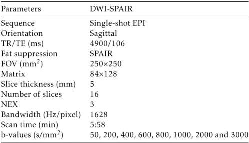
3.1 Sequence details for acquisition of the DWI images that were tested. . . 28 3.2 Scaling factors for each map on matlab in order for the maps to be correctly
L i s t o f S y m b o l s
θ Statistical dispersion of the distribution.
κ Probability distribution shape.
σ Width of the distribution.
α Stretching parameter.
D Pure diffusion coefficient.
DDC Distributed diffusion coefficient.
D∗ Perfusion-related incoherent microcirculation.
MD Mean diffusity type.
MK Mean kurtosis.
S1 Diffusion coefficients < 1×10⁻³mm2/s typical in tumor cells with restricted diffusion.
S2 Diffusion coefficients > 1×10⁻³mm2/s and < 3×10⁻³mm2/s water diffusion in other
components not mentioned inS1 andS3..
S3 Diffusion coefficients < 3×10⁻³mm2/s which represents the perfusion.
A c r o n y m s
CLUT Color Look Up Table.
DKI Diffusion Kurtosis Imaging.
DNA Deoxyribonucleic Acid.
DWI Diffusion Weighted Imaging.
EPI Echo planar imaging.
IVIM Intravoxel Incoherent Motion.
MRI Magnetic Ressonance Imaging.
PDF Probability Distribution Function.
ROI Region Of Interest.
C
h
a
p
t
e
r
1
I n t r o d u c t i o n
1.1 Context and motivation
Breast cancer is the second most common type of cancer that affects women and is the
second cause of death by cancer [1]. In Portugal only, there are 1500 women dying from this disease [2]. Pacients with history of benign breast tumors, early menarche, late menopause, use of oral contraceptives, hormone replacement therapy, high breast density and obesity have a higher risk of contracting the disease [3, 4].
With improved therapeutic and imaging techniques, in the last decades the breast cancer mortality rate has decreased substantially [5].
The Magnetic Ressonance Imaging (Magnetic Ressonance Imaging (MRI)) of the breast is an important medical imaging technique since it is the most sensitive method to detect invasive breast cancer in comparison with mammography and ultrasound [6]. It is based on the magnetic properties of the hydrogen nucleus in biological tissues and it provides multiplanar images of the breast [7]. It is used to detect breast cancer in high-risk patients for example, patients with mutations on the BRCA1 and BRCA2 genes. These genes are both tumor suppressing genes and their proteins are evolved in fundamental cellular processes, including the repair of double strands ruptures of Deoxyribonucleic Acid (DNA) [6]. In spite of only being responsible for 2% of all breast cancers, in case of the person having those gene mutations, the chances of someday contracting the disease are between 45% and 65% [6][8].
conventional methods. It is proven that, in this case, are detected malignant tumors that were hidden in mammography in approximately 3% to 9% of those women [10]. It is important to highlight that MRI can’t be performed on its own, but in conjuction with mammography since 12% of breast cancers, like carcinomas, can’t be detected by this imaging technique[11].
Diffusion Weighted Imaging (DWI) is a MRI technique based on the movement of
water molecules in tissues. The main goals of this technique are the study of lesion characterization and better detection of small size lesions [12]. There are several exten-sions of DWI, like for example diffusion kurtosis imaging (DKI). This extension assumes
that the water molecules movement doesn’t follow a Gaussian Probability Distribution Function (PDF). Biological tissues have natural barriers that are going to restrict the water molecules movement, thus diverting the PDF form from Gaussian. Kurtosis has the ability to identify how much the PDF diverts from the Gaussian shape, which gives information about the complexity of the tissues helping in lesion characterization [13]. Apart from the DKI, other non-Gaussian models have been studied for breast, like the Intravoxel Incoherent Motion (IVIM), and the Gamma distribution model [14, 15]. Other models like the Truncated Gaussian distribution and Stretched-Exponential model have also been studied for DWI, however only for prostate and brain tissues [16, 17, 18]. All of these models have been proven to differentiate between malignant and benign lesions
or normal tissue and lesions.
1.2 Objectives
This dissertation aims to develop a plug-in for OsiriX, which is a medical imaging clinical software. The purpose of the plug-in is to identify in a magnetic diffusion weighted image
whether a tumor is benign or malignant through the non-Gaussian models of diffusion
already existing and apply them to real images of the breast. The development of the plug-in was accomplished at Instituto de Biofísica e Engenharia Biomédica (IBEB).
1.3 Dissertation plan
The present dissertation has been structured so as to first cover relevant theoretic under-pinnings of diffusion MRI and non-Gaussian models. It also includes the state-of-the-art.
1 . 4 . D I S S E R TAT I O N O U T P U T S
1.4 Dissertation outputs
C
h
a
p
t
e
r
2
T h e o r e t i c U n d e r p i n n i n g s
In this chapter, the theoretic concepts are being introduced that are needed to better understand the state-of-the-art and remaining chapters of this dissertation. Firstly there is a small section about the breasts anatomy and the differences between malignant and
benign lesions. Then there is a brief introduction to MRI and DWI. The models that differ
from DWI are presented next and are divided in two sections, the Non-Gaussian models and the Statistical distribution models. The Non-Gaussian models explain the DKI and IVIM models and the Statistical distribution models explain the Gamma, Truncated and Stretched models. Afterwords, there is the State-of-the-art with the investigation done with each model applied to breast, with the exception of Truncated and Stretched which have not been applied to breast yet.
2.1 Breast anatomy
Macroscopically, the breast can be divided in two main parts. The first one is the glandular tissue, which is responsible for the production of milk. The second part are all of the other tissues that form and support the breast, which include adipose tissue (fat), fascia (connective tissue) and muscles, as shown in Figure 2.1 [19].
Figure 2.1: Anatomy of the breast. The female breast is constituted mainly of lobules (milk-producing glands), ducts (tubes that carry the milk from the lobules to the nipple), and stroma (fatty tissue and connective tissue surrounding the ducts and lobules, blood vessels, and lymphatic vessels). Adapted from [20]
categorized according to how many layers of cells are present and how atypical the cells appear. That way, it can range from atypical ductal hyperplasia to ductal carcinoma in situ. One barrier that prevents the spread of cancer is the epithelial layer. When this layer is breached, a carcinoma is labeled as invasive [19].
2.1.1 Benign vs Malignant lesions
Benign breast tumors tend to have a soft consistency and are mobile. Since they are slow-growing masses with a clear delimited margin or may be encapsulated their removal is easy and they rarely recur after removal. On the other hand, malignant tumors have irregular margins and are fast growing. They have an abnormal cell growth and can invade or spread to other parts of the body which defines them as cancer [21].
Although most benign tumors are not life-threatening, they have the potential to become malignant through tumor progression which is when there is an increase of the growth speed and invasiveness of the tumor cells [21].
2.2 MRI
2.2.1 Diffusion and MRI
2 . 2 . M R I
fat, to produce detailed anatomic images. A hydrogen nucleus is formed by only one proton which the axis, in the presence of a strong magnetic field, are forced to align either with or against the direction of the applied field. These two directions of alignment are a result of the existence of two possible energy levels that the protons can occupy inside a magnetic field. Since one of the levels has less energy than the other, the level with the lowest energy is going to have a number of protons higher than the level with the highest energy; this difference causes the net magnetization to be different from zero [22]. The
frequency at which protons precess when a magnetic field is applied is determined by
ω0=γB0 (2.1)
whereω0is the Larmor frequency,γ is the gyromagnetic ratio of the atom andB0is the magnitude of the applied magnetic field [23]. When radiofrequency energy at the Larmor frequency is applied, in a direction perpendicular toB0, the magnetic vector is deflected causing the hydrogen nuclei to resonate. Subsequently, the magnetic vector is going to release the energy that was absorbed and returns to its resting state at a rate defined by the T1 and T2 relaxation times. As shown in Figure 2.2, a radiofrequency pulse of 90◦is going to make the longitudinal magnetization in the tissue (vertical vector) become transverse (horizontal vector). Several radiofrequency pulses can be applied in order to emphasize the signal in the images, which happens as result of different tissues
relaxing at different relaxation rates. Therefore, T1 will represent the amount of time
that it takes for the magnetization to recover and align in the direction of the magnetic field, depending on the tissue in question, and T2 will be the duration of the transverse magnetization as protons wobble around the field. Due to heterogeneities of the local field, the protons wobble at different rates and the magnetic moment vectors of individual
proton magnetic resonance signals begin to cancel each outher out. The intensity of the signal will diminish as the transverse magnetization disappears [22].
2.2.1.1 MRI and the Breast
MRI was proposed as a method to detect breast cancer in 1970. This discovery showed that T1 and T2 relaxation times of abnormal breast tissue were considerably different
from normal tissue [5]. The contrast between tissues like fat, glandular tissue, lesions, etc, depends on the mobility and magnetic environment of the hydrogen atoms in the water and fat. These aspects define the intensity of the tissue signal in the image, which makes the parenchima, fat and lesion, in case of being present, even more evident [9]. Later, it was demonstrated that most breast cancers show a higher signal on T1- weighted images after the administration of gadolinium-based contrast [5]. This technique is highly sensitive (sensitivity between 71% and 100%). However, it is not enough to predict with precision which are the malign tumors, which means that it is necessary to resort to an invasive method called biopsy. Therefore, it became necessary to develop new non-invasive methods capable of predicting the histologic nature of the lesions [24].
2.2.1.2 Ultrasound and Mammography
The ultrasound imaging is the standard reference for differentiating between cysts and
solid masses. However, this examination may lead to false results, specially in the absence of discrete mass. Since is difficult to distinguish between malignant and benign lesions
due to ultrasound overlapping, biopsies are necessary, which in 70 % to 90 % of the cases have been proven to be unnecessary due to being benign tumors [7].
Mamography is the primary diagnostic tool for detection of breast cancer. However, its biggest disadvantage is that the produced image is two-dimensional, being the third dimension the thickness of the breast. This is projected onto a single plane, which can cause cancers to be obscured by overlying tissue, particularly in high-density breasts. The mammography in conjunction with the ultrasound imaging can increase the success rate in cancer detection by 50% [7].
It has been shown that MRI has higher sensitivity than 2D mammography which made it into a screening tool that can contribute in the early detection of cancer, specially in high-risk patients. However, it can’t be performed by its own, but in conjuction with mammography since 12% of breast cancers, like carcinomas, can’t be detected by this imaging technique[11].
2.2.2 Diffusion
In order to better understand how diffusion MRI works, it is useful to understand the
physical principles of water diffusion. This phenomenon was seen for the first time by
2 . 2 . M R I
He showed that this random motion of the water molecules could be described by a Proba-bility Distribution Function (PDF) which, in the absence of flow or barriers, is a Gaussian distribution centered around zero [25]. This means that the probability for a molecule to travel a short distance, or even not to move, is higher than the probability to travel a longer distance [26]. Therefore, the higher the mobility of the water molecules, the wider the Gaussian distribution will be [25].
2.2.3 Diffusion Weighted Imaging
DWI is a MRI technique that is non invasive and that allows the characterization and quantification of the molecular water diffusion in tissues [27]. It is typically performed
using a T2 weighted spin-echo prepared Echo planar imaging (EPI) sequence, that is used due to its short acquisition times, which minimizes movement artifacts [28]. The diffusion preparation module uses two gradients that allow to measure diffusion. The
first gradient pulse changes the magnetization of every water molecule, while the second gradient pulse completely removes this alteration, which will only happen as long as the water molecule remains at its original location. However, if moving spins experience an incomplete rephasing between diffusion gradients, it will lead to a diffusion-dependent
signal attenuation. This means that if the water molecule makes any movement when these pulses are applied, it will lead to incomplete restoration of the water magnetization causing a decrease of the MR image signal. The loss of diffusion signal is controlled by
thebvalue. The greater the mobility implies less MRI signal [29]. Thebvalue parameter is given by Equation 2.2:
b=γ2G2δ2(∆−δ/3) (2.2)
whereγ is the proton gyromagnetic ratio, G is the gradient strength,δis the duration of the gradient and∆is the time between the application of the two diffusion gradients,
as indicated in Figure 2.3 [30].
The magnetic resonance signal is reduced in intensity proportionally to water mobility. This is described by the Equation 2.3. WhereS(b) is the intensity of the signal for different
bvalues andS(0) is the intensity of the signal for a zerobvalue, or in other words, when there isn’t a diffusion gradient applied [28].
ln[S(b)] = ln[S(0)]−bADC (2.3)
Thebvalue is then used to estimate the for each voxel of the image [31]. In general, the Apparent Diffusion Coefficient (ADC) is defined as the surface area that delimits
the volume that the water molecules can occupy, having into account the displacement during a certain period of time (∆). It depends strongly on the interaction of the water
molecules with its adjacent structures, rather on intrinsic diffusion properties [30].
The standard diffusion sequence can generate two types of images (Figure 2.4). The
Figure 2.3: Pulse sequence diagram of a spin eco sequence. There are two diff
usion-sensitizing gradients inserted before and after a 180º radiofrequency refocusing pulse. The important factors that define the degree of diffusion-sensitization are the gradient
amplitude (G), duration (δ), and the time between the two sensitizing gradients (∆)[28].
and the second are images that reflect the water mobility, which are diffusion weighted
obtained with diffusion gradients (S(b)). Diagnostic information can be disguised by long
T2 signal, that is an artifact also known as "T2 shine through". The parametric ADC map is created in order to facilitate diffusion quantification, since it doesn’t have the T2 shine
through effects. In Figure 2.4 it is also possible to deduce that an area with restricted
diffusion is more intense in a weighted image than in an ADC map [28]. Therefore, the
ADC value decreases in the presence of malign tumors, since the bigger cellular density that exists in the tumoral tissue, in comparison with normal tissue, restricts the diffusion
of the water molecules, which means that the ADC value can be used to detect and monitor the tumor [31].
Previous studies have shown a decrease on the number of false positive results with the DWI technique, having a sensitivity of 84% and a specificity of 79% [5]. However, this model is based on the assumption that the environment is homogeneous and since sometimes the benign and malign lesions can’t be distinguished due to the overlap of their diffusion coefficients, there is a need to develop techniques that offer a better
char-acterization of breast cancer tissues in a way to assist the classification and differential
2 . 3 . N O N - G AU S S I A N M O D E L S
Figure 2.4: Examples of images obtained with DWI. A isS0withb= 0s/mm2and B isSb
withb= 800s/mm2. Image C is anADCmap. The arrow points towards a tumor that in A and B appears hyperintense and in C appears hypointense, exhibiting low diffusion [28].
2.3 Non-Gaussian Models
2.3.1 Diffusion Kurtosis Imaging
The DWI model is able to characterize the average diffusion displacement of the water
molecules in a three-dimensional space. However, it is not capable to provide specific information about the environment in which the water spins are located. That means that it is able to evince the shortness of the water diffusion distance, but it can’t substantiate if
the short distance is due to a more viscous environment or due to the presence of biologi-cal barriers like cellular membranes [32]. Thus, these techniques have some limitations, such as assuming that water diffusion follows a Gaussian distribution. It has already
been proven that these models are not enough to characterize biological tissues because of barriers and compartments that restrict the water movement. This deviation from the Gaussian behavior can be quantified through the use of a non-dimensional metric called excess kurtosis, or kurtosis. Because the deviation from the Gaussian movement changes with the complexity of the tissue, kurtosis is a direct measure of the degree of tissue complexity [13, 33, 34, 35].
small displacements than hindered diffusion. On the other hand, if K has a negative value,
the tails of the distribution are wider and its peak lower, which means that the probability of small displacements would be lower than Gaussian diffusion, which is not expected
in biological tissues since there isn’t fully restricted diffusion. In spite of K being able
to be positive or negative, in biological tissues K has been shown to have only positive values since one rather expects the imaged volume to consist of a mixture of hindered and restricted compartments [25].
Figure 2.5: Probability distributions with the variation of kurtosis values [25].
The Diffusion Kurtosis Imaging (DKI) is an extension of the DWI model introduced by
Jensen and Helpern in 2005 [13, 34, 36]. This model includes the kurtosis and diffusion
coefficients and their estimation requires the use of highbvalues, that increase the
dura-tion of the exam in order to observe the non-Gaussian behavior of the water molecules diffusion[13, 36].
ln[S(b)] = ln[S(0)]−bMD+1 6b
2MD2MK+O(b3) (2.4)
In order to obtain the kurtosis diffusion parameters, the equation (2.4) is used, where
MDis the average diffusion,MKthe average kurtosis andO(b3) the error associated with
the measurement. Both equations ((2.3) and (2.4)) are identical when MK is similar to zero and theADCis similar toMD[13]. It should be noticed that unlike what occurs in equation 2.3, the kurtosis variable in equation 2.4 appears as part of a term depending onb2, which means that the signal won’t decay linearly with thebvalue [25]. WhenMK
2 . 3 . N O N - G AU S S I A N M O D E L S
2.3.2 Intravoxel Incoherent Motion
An important aspect of diffusion MRI is its sensitivity to perfusion since the flow of blood
water in randomly oriented capillaries is similar to diffusion – named intravoxel
incoher-ent motion (IVIM) effect [37]. IVIM is a technique that uses low b-values (i.e., 0–1000
s/mm2) DWI to separate the estimation of tissue perfusion and diffusivity, followed by
biexponential curve fitting [14]. At lowbvalues (e.g., 100 s/mm2), the measured signal attenuation comes from not only the water diffusion in tissues, but also from
microcircu-lation in capillaries [38].
This type of diffusion depends on the displacement speed of the flowing blood, the
vascular architecture and thebvalues, which affect the signal attenuation in each imaging
voxel. However, the amount of signal attenuation from pseudo-diffusion
(microcircula-tory perfusion of blood within capillaries with no specific orientation) is bigger than tissue diffusion due to the large distances of proton displacement while motion-probing
gradients are being applied. This means that at lowb values, pseudo-diffusion has a
relatively high contribution to the DW-MRI signal and at highb values it accounts for only a small proportion [38].
Figure 2.6 shows a plot of signal attenuation of a well-perfused tissue (liver parenchyma) with increasingbvalues from a healthy person. It is possible to see in the figure that there is a steeper slope of signal attenuation when thebvalues are low. Since protons in flowing blood have larger diffusion distances and the signal is attenuated by small weightings (e.g.,
<100 s/mm2), the steep slope can be justified by microcapillary perfusion. When largerb
values (e.g., >100 s/mm2) are being applied, the signal attenuation of the perfusing pro-tons is almost complete, hence microcapillary perfusion will have a lower contribution to the signal. Therefore, in figure 2.6, at largerbvalues the slope of signal attenuation is less steep and is more reflective of tissue diffusity [38].
Consequently, from the IVIM model is possible to obtain the following parameters: pure diffusion coefficient (D), perfusion-related incoherent microcirculation (D∗), which
is considered proportional to the mean capillary segment length and average blood veloc-ity, and microvascular volume fraction (f) as it is shown in Equation (2.5) [14].
S(b)
S(0)= (1−f)exp(−bD) +fexp[−b(D
Figure 2.6: The plot shows the logarithm of relative signal intensity versusbvalue from normal liver parenchyma from an healthy 30-year-old man. Within the A box there is a decrease in plotted signal values at low b values in comparison with a more grad-ual attenuation of signal at higherb values (box B). By applying intravoxel incoherent motion (IVIM) analysis, it is possible to obtain the signal attenuation biexponential behav-ior (solid line), while by using a simple monoexponential apparent diffusion coefficient
(ADC) line fitted to the data (dotted line), a suboptimal characterization of the signal is obtained[38].
2.3.2.1 Intravoxel Incoherent Motion and Diffusion Kurtosis Imaging
Iima et al. [37] explored the potential of non-Gaussian diffusion and perfusion MRI. Since
IVIM is used with lowbvalues and DKI with highbvalues, both models were taken into account, creating an updated quantitative imaging framework.
When both models are joined, the final equation (Equation 2.6) is:
S(b) =S(0)fIV IMexp(−bD∗) + (1−fIV IM)exp[−bADC0+ (bADC0)2K/6] (2.6)
where, as it was referred before in 2.3.2,S(0) is theoretical signal whenbis equal to zero;fIV IM the (T1-,T2- weighted) volume fraction of incoherently flowing blood in the tissue; D∗ perfusion-related incoherent microcirculation associated to the IVIM effect;
ADC0which is theADCvalue when thebvalue approaches zero.K is the dimensionless kurtosis coefficient which characterizes the deviation from the Gaussian behavior and,
2 . 4 . S TAT I S T I CA L D I S T R I B U T I O N M O D E L S
2.4 Statistical distribution models
2.4.1 Gamma Distribution
The Gamma distribution model is based on a statistical approach that can be related to heterogeneous tissues considering that tumor tissue is a mixture of different tissues and
perfusion components. It works by assuming that each tissue component has a certain
ADCthat matches a part of theADC distribution [15, 39].
Figure 2.7: Gamma distribution of five curves, each with different parameters values.
When the shape parameterκand the scale parameterθchanges, the distribution shape varies significantly [39].
This model has two main parameters that define the distribution: theθparameter, which shows the statistical dispersion of the distribution, and theκ parameter, that is responsible for the probability distribution shape [15, 39]. In Figure 2.7, the effect of the
parameters on the distribution curves is clear. The distribution is given by Equation 2.7:
ρ(D) = 1
Γ(κ)θκD
κ−1exp−D
θ
(2.7)
whereΓis the gamma function and D, the diffusion coefficient. When the diffusion
coefficient is distributed according to this function, we obtain the following equation:
S(b) =S(0)
Z ∞
0
ρ(D)exp(−bD)dD=S(0) 1
whereb is the b value. Theθ andκ can be estimated by curve-fitting of magnetic resonance diffusion data that is obtained by using multiplebvalues [39].
2.4.2 Truncated Gaussian Distribution
The truncated Gaussian distribution is a statistical model that reflects the consequences of a distribution of length scales for restrictions and hindrances to water diffusion, through
a diffusion coefficient probability distribution which is defined by a mean value and a
distribution width. This model assumes that a given voxel containing several cells, and intercellular and extracellular spaces, can be described as a sum of different spin packets.
These packets have differentADC values since they originate from different positions,
went through different trajectories and faced different restrictions and hindrances to
displacement [40]. Under these assumptions, the signal can be described by Eq (2.9):
S=S0exp
−bADC+1 2σ
2b2 (2.9)
whereσ is the width of the distribution. This model is able to fit the data with only two free parameters (ADC andσ) that can quantify the diffusion heterogeneity by the
width of the distribution of diffusion rates [18]. This model has not yet been applied to
breast MRI.
2.4.3 Stretched-Exponential Model
The stretched-exponential model was first described by Bennet et al. [41] for brain imag-ing. It was presented as an alternative to the biexponential model of water diffusion
that assumed the existence of two different proton pools inside of each voxel, which had
different diffusion rates resulting in signal relaxation. The stretched-exponential model
makes no assumption on the number of intravoxel proton pools, proposing that the signal attenuation came from a collection of uncoupled exponential decay processes, resulting in the following equation (2.10) :
S(b)
S(0)=
Z ∞
0
ρ(D)e−bDdD (2.10)
which when described as a function of b results in equation (2.11):
S(b)
S(0)= exp{−(b×DDC)
α} (2.11)
whereα is the stretching parameter, which relates to intravoxel water diffusion
het-erogeneity, andDDCis the distributed diffusion coefficient, which represents the mean
intravoxel diffusion rates [41, 42]. Theα parameter varies from zero to one. When it
is close to one, it indicates that the apparent diffusion has high homogeneity, or
mono-exponential diffusion-weighted signal decay. Inversely, if it is close to zero, it indicates
2 . 5 . S TAT E - O F -T H E -A R T
to refer that when heterogeneity is mentioned in this model, it refers to intravoxel hetero-geneity of exponential decay and not to intervoxel heterohetero-geneity of diffusion coefficients).
TheDDC can be considered to be an individualADC approximation weighted by the volume fraction of water in each part of the continuous distribution ofADCs[17, 41, 42].
This model has the ability to give an accurate description of the water diffusion in
tis-sues since it is able to fit a variety of observed decay shapes using only two fit parameters [42].
2.5 State-of-the-art
Several studies have been made on the non gaussian models mentioned previously. In spite most of the models having been applied to breast, two of them have only been applied to the brain and the prostate (truncated and stretched models). In this section the reader will be able to see the results from the studies applied to these models. All of these models have proven to successfully detect malignant tumors being the reason for why they were adapted to produce parametric maps in this plugin.
2.5.1 State-of-the-art of Diffusion Kurtosis Imaging
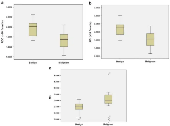
Nogueira et al. [13] concluded in their study that there are significant differences between
theMDandMK lesion types when the DKI model is applied. As is seen in Figure 2.10 and in Table 2.1,MK values are lower for benign lesions than for malignant lesions and
MDvalues are higher for benign lesions than for malignant lesions [13]. This decrease ofMD and increase of MK can be explained by the increase of cellularity observed in malignant tumors. If there are less barriers, like in the case of benign tumors, the diffusion of water molecules will be easier, thusMDvalues will be higher and theMK
values will be lower, since it is approaching a Gaussian profile which is a characteristic of homogeneous environment. According to a study directed by Wu et al. [27] the sensitivity forMDandMKis respectively 79,3% and 84,2%. As for the specificity is 92,9% for both parameters. Wu also compared the results through parametric maps seen in Figure 2.8 of a patient with malignant carcinoma – infiltrating ductal carcinoma. In (a) and (b) shows a T2- weighted TSE image and a DW image whenbis equal to zero where the lesion is easily seen. In (c) the lesion is seen darker, meaning that theMD values are lower and in (d) the lesion is seen lighter, which means that it has higher values ofMK. These results are consistent with a malignant tumor. In Figure 2.9 shows also in a) and (b) a T2- weighted TSE image and a DWI image whenbis equal to zero where the lesion is easily seen. In (c) the lesion is seen lighter, meaning that theMDvalues are higher, and in (d) the lesion is seen darker, which means that it has lower values ofMK. Therefore, the same conclusion is reached as in Figure 2.8, that these results are consistent with a benign tumor.
Table 2.1: ADC (apparent diffusion coefficient), MD (mean diffusity) and MK (mean
kurtosis) parameters obtained by the two models of DWI (mono-exponential and diffusion
kurtosis), and differences by lesion type [13]
Mean Benign (n=13) Malignant (n=31) p*
ADCa 1.96±0.41 1.33±0.43 0.017
MDa 2.17±0.42 1.52±0.50 0.028
MKb 0.37±0.18 0.61±0.27 0.017
aADCandMD(×10−3mm2/s) bMK is a dimensionless metric
*Statistical differences
Figure 2.8: The white arrow indicates a malignant carcinoma (infiltrating ductal carci-noma) of a 51 year-in-old woman: a) T2-weighted Turbo spin echo (TSE) image; b) DW image at b=0; c)MD- mean diffusion map; d)MK - mean kurtosis map [27].
2.5.2 State-of-the-art of Intravoxel Incoherent Motion
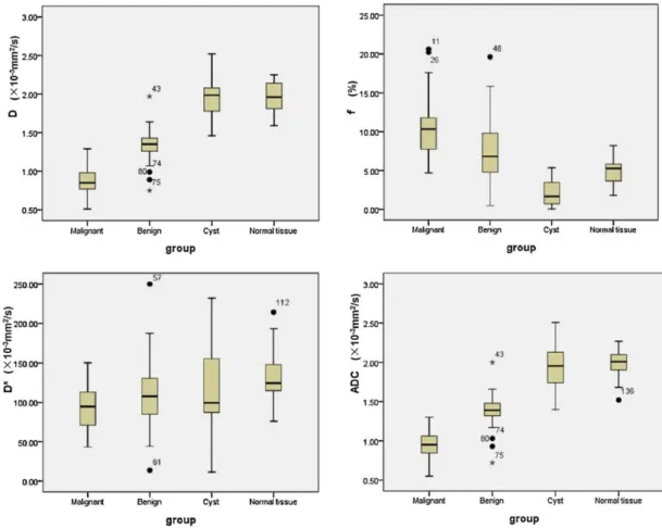
Liu et al. [14] found thatDvalues of malignant tumors were significantly smaller that those of benign lesions, cysts and normal breast tissues, as seen on Table 2.2 and on Figure 2.11. Also, theADCvalues andDvalues between malign and benign tumors were different, concluding that the microperfusion effect did add information to theADCvalue.
Thef values were higher in malignant tumors which supported the theory that malignant tumors have higher vascularity. This observation, in combination with the lowDvalue, strongly suggests the presence of a malign lesion. In the mean time, (D∗) did not show any significant differences between malignant and benign lesions, which may be caused by the
varying vascularity among different tumor types. In Figure 2.11 there is also a comparison
of the parameter values between malignant, benign, cyst and normal tissue. However, cyst, malignant, benign and normal tissue do not show significant differences. While
in the malignant, benign and normal tissue, the parameters had significantly different
2 . 5 . S TAT E - O F -T H E -A R T
Figure 2.9: The white arrow indicates a benign lesion (fibroadenoma) of a 56 year-in-old woman: a) T2-weighted Turbo spin echo (TSE) image; b) DW image at b=0; c)MD- mean diffusion map; d)MK - mean kurtosis map [27].
Table 2.2: Values of pure diffusion coefficient (D), microvascular volume fraction (f),
perfusion-related incoherent microcirculation (D∗) and apparent diffusion coefficient
ADCof malignant and benign breast lesions [14].
Malignant tumors (n = 40) Median (quartiles)
Benign lesions (n = 41) Median (quartiles) p
D(×10−3mm2/s) 0.85 (0.77, 0.98) 1.35 (1.26, 1.44) 0.000
f(%) 10.34 (7.68, 11.88) 6.83 (4.72, 10.33) 0.000
D∗(×10−3mm2/s) 94.71 (70.33, 113.23) 107.49 (83.20, 131.19) 0.000
ADC (×10−3mm2/s) 0.95 (0.83, 1.06) 1.39 (1.32, 1.50) 0.000
Table 2.3: Sensitivity and specificity of IVIM parameters [14].
Sensitivity (%) Specificity (%)
D(×10−3mm2/s) 90 92.68
f(%) 87.50 53.66
D∗(×10−3mm2/s) 85.00 41.46
ADC(×10−3mm2/s) 92.50 90.24
2.12 and Figure 2.13) which were in agreement with the results already mentioned. In the figures, theD,ADC andf maps, are darker for the malignant lesion, which means that it has low values, and brighter for the benign lesion, which means that it corresponds to higher values. The specificity and sensibility of the models are shown in Table 2.3.
According to a study for prostate cancer, thef values were significantly increased in tumors withb values below 800 s/mm2. However, the f values became lower or indistinguishable from normal tissues with high b values [44]. Meaning that to obtain good parametric values, the images used can’t have a biggerbvalue than 800 s/mm2.
Figure 2.10: Box plot distribution of the parameters by lesion type ofADC(a) parameter using the mono-exponental model, andMD(b) andMK(c) parameters using the kurtosis model.MK is a dimensionless metric [13]
contributions made the differentiation between normal and malignant lesions more eff
ec-tive than with onlyADC values. However, both works presented limitations. They had a small population of patients to examine which made the comparison between results more challenging. Another important limitation is the unknown suitable number of b
values for breast IVIM (varying from six to ten in previous studies) making the selection ofbvalues and reduction of their number crucial for an optimal procedure.
2.5.2.1 State-of-the-art of Intravoxel Incoherent Motion Diffusion Kurtosis Imaging
The results obtained by Iima et al. [37] are shown in Table 2.4. In order to show differences
from non-Gaussian models and Gaussian models, the authors also compared the values obtained from the IVIM/DKI models with the ones from standard mono-exponential mod-els (ADCmono andf IV IMmono). In malignant lesions, theK (dimensionless parameter)
was significantly higher andADC0lower than that in benign lesions. AlthoughADCmono
also showed differences between malignant and benign tumors or normal tissue, they
were always smaller thanADCmono values. f IV IM had higher values in malignant
tu-mors than that in benign tutu-mors andD∗andf IV IMmonoshowed no significant difference
2 . 5 . S TAT E - O F -T H E -A R T
Figure 2.11: Box plots in breast lesions and normal tissue ofD(a),f (b),D∗(c) andADC
(d). The line in a box represents median value [14].
In conclusion, both diffusion and perfusion parameters from this model were able to
differentiate between malignant and benign tumors with high sensitivity and specificity.
Which means that this study was able to estimate diffusion and perfusion parameters
in one step [37]. However, the fitting approaches (such as the Marquardt-Levenberg algorithm) used to estimate the parameters, are very sensitive to noise. In order to resolve this issue, the equation is often divided in two steps. First estimating the diffusion
parameters and then the perfusion parameters from the residual signal. Nonetheless, it assumes that the IVIM perfusion effects don’t contribute to signal forb values above
a certain cutoff value, which is not the case in spite of having a smaller contribution.
Another drawback, is sensitivity of the algorithm towards the set of initial parameters that are required for the fitting process to begin. And like the other models, the population size in which the tests were made was very small [37].
2.5.3 State-of-the-art of Gamma Distribution
Figure 2.12: Parametric maps of a 25-year-old woman with a fibroadenoma(thin arrow) and a simple cyst in her left breast (thick arrow): pure diffusion coefficient (D),
mi-crovascular volume fraction (f), perfusion-related incoherent microcirculation (D∗) and apparent diffusion coefficientADC [14].
Table 2.4: Values of apparent diffusion coefficient when the b values approaches zero
ADC0, kurtosisK, a dimensionless parameter, apparent diffusion coefficient of a mono-exponential modelADCmono, the volume fraction of incoherently flowing bloodf IV IM, perfusion-related incoherent microcirculationD∗and the volume fraction of incoherently flowing blood using a mono-exponential modelf IV IMmono[37].
Parameter Malignant Benign p
ADC0(×10−3mm2/s) 1.05 (0.94–1.17) 1.73 (1.51–1.94) <0.001
K 0.82 (0.70–0.94) 0.55 (0.42–0.68) <0.05
ADCmono(×10−3mm2/s) 1.00 (0.88–1.11) 1.50 (1.35–1.66) <0.001
f IV IM% 12.3 (8.86–15.7) 5.00 (0.60–9.40) <0.05
D∗(×10−3mm2/s) 10.9 (5.95–15.9) 13.9 (5.96–21.9) 0.52
f IV IMmono% 8.63 (7.39–9.86) 8.66 (6.97–10.4) 1.00
have high values, the distribution will be more expanded; whenκ is smaller, the shape of the distribution will be more altered. For benign tumors it would be the other way around,θwill be lower, the distribution will be more compressed, andκwill be higher and the shape of the distribution will be less altered [39].
2 . 5 . S TAT E - O F -T H E -A R T
Figure 2.13: Parametric maps of a 30-year-old woman with invasive ductal carcinoma: b: IVIM parametric maps of pure diffusion coefficient (D), microvascular volume fraction
(f), perfusion-related incoherent microcirculation (D∗) and apparent diffusion coefficient
(ADC) maps [14].
Table 2.5: Values of the Gamma distribution parameters: the statistical dispersion of the distributionthetaand the probability distribution shapeκ[15]
Parameters Malignant Benign
θ(×10−3mm2/s) 1.23±0.52 4.29±1.90
κ 0.97±0.50 0.65±0.43
presence of tumor cells with restricted diffusion. Also, if theADCvalues are larger than
3.0 mm2/s it can happen due to perfusion and if they are between those two values, it is attributed to water diffusion in the other components. This way, for clinical evaluation,
two fractional areas were evaluated. With frac < 1 (D < 1.0 mm2/s) and frac > 3 (D > 3.0 mm2/s) like is shown in Figure 2.14.
The results that were obtained and shown in Figure 2.15 were from prostate DWI images. In Image a), the cancer group (ca) and non cancer group (PZ) are distinct and separated. Unlike Image b) which the separation is not clearly visible [39].


![Figure 2.15: a) Scatter plot of frac>3 vs frac<1; b) Scatter plot of θ vs κ; for the cancer and not cancer group [39].](https://thumb-eu.123doks.com/thumbv2/123dok_br/16541286.736743/50.892.165.761.561.848/figure-scatter-plot-frac-scatter-cancer-cancer-group.webp)