FUNDAÇÃO GETULIO VARGAS
ESCOLA BRASILEIRA DE ADMINISTRAÇÃO PÚBLICA E DE EMPRESAS
MESTRADO EXECUTIVO EM GESTÃO EMPRESARIAL
OIL PRICES EFFECTS ON COLOMBIA’S MAIN
MACROECONOMIC INDICATORS
LUIS FERNANDO MALDONADO UMAÑA
Rio de Janeiro - 2016
DISSERTAÇÃO APRESENTADA À ESCOLA BRASILEIRA DE ADMINISTRAÇÃO PÚBLICA E DE EMPRESAS PARA OBTENÇÃO DO GRAU DE MESTRE
Ficha catalográfica elaborada pela Biblioteca Mario Henrique Simonsen/FGV
Maldonado Umaña, Luis Fernando
Oil prices effects on Colombia's main macroeconomics indicators / Luis Fernando Maldonado Umaña.– 2016.
64 f.
Dissertação (mestrado) - Escola Brasileira de Administração Pública e de Empresas, Centro de Formação Acadêmica e Pesquisa.
Orientador: Istvan Karoly Kasznar. Inclui bibliografia.
1.Administração de produtos. 2. Petróleo - Colômbia. 3. Petróleo - Derivados - Preços. 4. Indicadores econômicos - Colômbia. 5. Indústria petrolífera - Colômbia - Modelos econométricos. I. Kasznar, Istvan Karoly. II. Escola Brasileira de
Administração Pública e de Empresas. Centro de Formação Acadêmica e Pesquisa. III. Título.
Table of Contents:
1 Introduction ... 9
2 Oil Price Behavior ... 10
2.1 2003-2008 Oil Price Rise and Plunge... 14
2.2 2014 Price Shock ... 16
3 Colombia Oil Market Overview ... 19
3.1 Colombia Oil Production ... 19
3.2 Oil Exports ... 20
3.3 Oil Imports ... 21
3.4 Trade Balance ... 22
4 Importance of Oil Prices in Colombian Economy ... 24
4.1 Current Account ... 24
4.2 Exchange Rate ... 25
4.3 Oil Production ... 26
4.4 Consumer Price Index (CPI)... 27
4.5 Gross Domestic Product (GDP) ... 28
5 Literature Review ... 30
6 Model Description ... 32
6.1 Vector Autoregression (VAR) Definition ... 32
6.2 Variables Description ... 33
6.3 Determining the Number of Lags in the Model ... 36
7 Results: ... 39
7.1 Descriptive Statistics: ... 39
7.2 Unit Root and Cointegration Tests ... 40
7.3 Impulse Response Results to a Shock in Oil Prices ... 42
7.4 Results Analysis ... 46
8 Conclusion and Recommendations ... 48
9 References: ... 49
10 Annexes: ... 51
10.1 Annex 1: Colombia’s Oil Production and Consumption ... 51
10.2 Annex 2: Colombia’s Oil Exports and Total Exports Data ... 52
10.3 Annex 3: Colombia’s Oil Imports and Total Imports Data ... 54
10.4 Annex 4: Colombia’s Oil Trade Balance and Total Trade Balance Account ... 55
10.5 Annex 5: Colombia’s Foreign Direct Investment (FDI) and Oil Prices ... 56
10.6 Annex 6: Monthly Oil Prices ... 57
10.8 Annex 8: USDCOP Exchange Rate or Tasa Representativa Del Mercado (TRM) . 60 10.9 Annex 9: Consumer Price Index (CPI) Information ... 61 10.10 Annex 10: GDP Quarterly Growth and Quarterly Oil Prices ... 63
Figures Index:
Figure 1: Demand ... 11
Figure 2: Supply ... 12
Figure 3: Demand and Supply ... 13
Figure 4: Oil Price Behavior 2003 - 2008 ... 14
Figure 5: World, China & India GDP Growth / Oil Supply & Demand Growth ... 15
Figure 6: Oil Price Behavior 2014 - 2016 ... 17
Figure 7: Colombia Avg Daily Oil Production and Consumption (thousands of barrels) ... 20
Figure 8: Colombia Monthly Oil Exports (Usd$ Millions) ... 21
Figure 9: Colombia Monthly Oil Imports (Usd$ Millions) ... 22
Figure 10: Comparison of “Oil Trade Balance” vs. Colombia’s Trade Balance Account ... 23
Figure 11: Foreign Direct Investment (FDI) and Oil Prices ... 24
Figure 12: TRM vs. WTI and Brent Prices ... 25
Figure 13: Colombian Oil Production vs. Oil Prices ... 26
Figure 14: WTI Prices vs. CPI Yearly Change ... 27
Figure 15: GDP Growth vs. Oil Prices ... 29
Figure 16: ISE Impulse Response Results ... 43
Figure 17: Inflation Impulse Response Results ... 43
Figure 18: Trade Balance Impulse Response Results ... 44
Figure 19: Repo Rate Impulse Response Results ... 45
Tables Index:
Table 1: Lag Tests Results ... 37
Table 2: R-Squared For Var(4) and Var(1) Models: ... 38
Table 3: Covariance and Correlation Analysis of Variables in the Model:... 40
Table 4: Other Descriptive Statistics: ... 40
Table 5: Unit Root Test Results ... 41
This research main purpose is to determine the effects of oil prices in an oil exporting economy with focus on the Colombian case. First of all, it will be determined if Colombia is a net oil exporter; then, the relevance of oil exports in Colombia’s economy will be determined in order to define if this commodity is important for the Colombian economy. After proving the importance of oil in the country’s economy, an econometric model will be applied to demonstrate if the hypothesis that there is a direct relationship between oil prices and Colombia’s economic performance is true. The variables that are going to be tested in this paper are Consumer Price Index (CPI), Gross Domestic Product (GDP) and Balance of Payments (BOP) which captures the net effect between exports and imports plus net capital flows.
If the hypothesis that oil prices directly affect Colombia’s economic performance is proved to be right, very close attention must be paid because oil is a non-renewable source of energy and unless new oil deposits are discovered, the commodity will begin to drain and an even higher negative effect can be observed in the future if the country’s economic focus doesn’t change before existing oil is all used up along with the county reserves. If the country doesn’t concentrate in diversifying its economy, Dutch disease can be very harmful because the economy will be in very bad shape when oil dries up or prices become very low that country revenues plummet and extracting this commodity is not profitable enough and production and further exploitation will simply be inexistent.
1 Introduction
Oil is a substance that has its origins in organic compounds primarily composed of hydrogen and carbon thus being part of the hydrocarbon family. It is from fossil origin and it is found inside the geological formations of the Earth.
Currently Oil is the world’s main source of energy being the energy input for almost all motorized vehicle such as cars, motorcycles, planes, boats and trains just to mention some. Oil is a worldwide traded commodity and its price fluctuates depending on supply and demand which at last determines its price. Crude oil price is set mainly by interactions of the many participants that are in the market, each with their own view of the commodity price. Crude oil prices vary depending of their type, which are categorized as light and heavy crude. Light crude oil is less viscous and given that flows easily requires less refining process to produce finished products such as gasoline. Heavy oil is much more viscous than light oil and often requires heat or diluents for it to flow; additionally, heavy oil, if processed identically as light crude produces higher amounts of residual oil and asphalt which are less valuable than main products such as gasoline. Crude oil is also categorized by the amount of impurities it has given that as more impurities are present, it is more difficult to refine. Main impurity present in oil is sulfur, so it is categorized on the amount of sulfur present; if crude presents low sulfur levels, it is categorized as sweet and if it has high sulfur levels is called sour.
Crude oil prices depend on the type of oil that is sold/bought; heavy and sour oil will be more expensive than light and sweet crude because the first requires a more complex process than the latter.
2 Oil Price Behavior
In economics it is well known that the price of any good or service is determined by the forces of supply and demand. To understand how prices are set, demand and supply will be defined separately and then will be brought together to explain how the price of a good/service is determined by these forces.
A lot has been debated whether if oil prices follow the demand and supply theory for fixing its prices and many of papers have been written determining whether if there are other variables exogenous to the theory that may play an important part in price formation.
A paper written by Javan and Vallejo explains the oil price changes observed between 2007-2009 and 2014-2015 and tried to determine if the futures market had an effect in oil prices. They concluded that “the main factor for the increase of the price in 2008 was the higher than expected demand. For the 2014 decline the VECM shows that supply is the main force behind it.”1 Hamilton in 2009 also concluded that oil “price run-up of 2007-2008 was caused by strong demand confronting stagnating world production.”2 Killian and Murphy (2011) also agreed that oil prices move according to the supply and demand theory concluding that 2003-2008 oil price “surge was caused by unexpected increases in world oil consumption driven by the global business cycle.”3 Taking the mentioned literature into account, it can be assumed that oil prices follow the supply and demand theory so 2008 and 2014 shocks will be explained by these forces.
Before explaining 2008 and 2014 oil shocks, a brief and simple description of demand and supply will be shared in order to help illustrate how prices are set.
Demand:
“The quantity demanded of any good is the amount of the good that buyers are willing and able to purchase.”4 Taking this definition as a starting point, we can infer that there are many factors that determine the demand of a good/service, but one of the most important (if not the most) is price. The willingness for consumers to purchase a good/service depends on the price according to the law of demand which states that “Other things being equal, when the price of a good
1 Javan, A., & Vallejo, C. (2016). Fundamentals, non-fundamentals and the Oil Price Changes in 2007-2009 and 2014-2015. OPEC Energy Review, 40(2). 125-154.
2 Hamilton, J. D. (2009). Causes and Consequences of the Oil Shock of 2007-08. Brookings Papers on Economic
Activity 2009(1). Brookings Institution Press.
3 Kilian, L., & Murphy, D. P. (2014). The role of Inventories and Speculative Trading in the Global Market for Crude Oil. Journal of Applied Econometrics, 29(3),454-478.
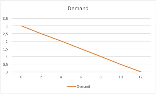
rises, the quantity demanded of the good falls, and when the price falls, the quantity demanded rises.”5 The relationship between price and demand can be obseved in Figure 1:
Figure 1: Demand
Figure 1 shows price in the Y axis and demand in the X axis. In this example law of demand is clearly explained since when price is $0, we observe that demand is the highest and when price reaches $3, the quantity demanded for this good/service becomes inexistent. There is an inverse relationship between these variables because as prices goes up, the demand for the good/service declines.
It must be taken into consideration that there are other factors that affect the demand such as income, price of substitute goods, number of buyers and buyer’s preferences just to mention some. These other factors may shift demand curve to the left or to the right depending if it positively or negatively affects the quantity demanded for the good/service being studied.
Supply:
Supply is viewed from the producer/seller point of view instead than from the consumer point of view as in demand. “The quantity supplied of any good or service is the amount that sellers are willing and able to sell.”6 As in demand, supply is also affected by the prices of goods/services in the market; the willingness of sellers/producers to sell a good/service depends
5Mankiw,N.Gregory,,. (2015). Principles of macroeconomics 6 Mankiw,N.Gregory,,. (2015). Principles of macroeconomics
0 0,5 1 1,5 2 2,5 3 3,5 0 2 4 6 8 10 12
Demand
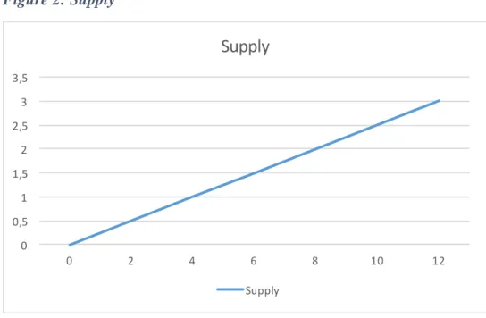
Demandon the market price at which they can sell. Taking this into account, the law of supply states that leaving other variables that may affect the supply, if the price of a given good/service raises, the producer/seller is willing to produce/sell more quantity of the item in question; if on the contrary, the price of the good/service falls, the producer/seller is willing to produce/sell less. Figure 2 illustrates this effect:
Figure 2: Supply
On Figure 2 price is in the Y axis and supply is in the X axis. In this example law of supply is clearly explained since when price is $0, we observe that supply is 0 and when price reaches $3, the quantity supplied for this good/service becomes is the highest. There is a direct relationship between the variables because as the price goes up, supply raises as well.
As in the demand curve, it must be taken into consideration that there are other factors that affect the supply such as the prices of raw materials used to produce the good/service, technology used to transform raw materials into a product/service, and number of sellers of he given product/service just to mention a few. These factors (and others not mentioned) may shift supply curve to the left or to the right depending if it positively or negatively affects the quantity supplied for the good/service being studied.
Demand and Supply:
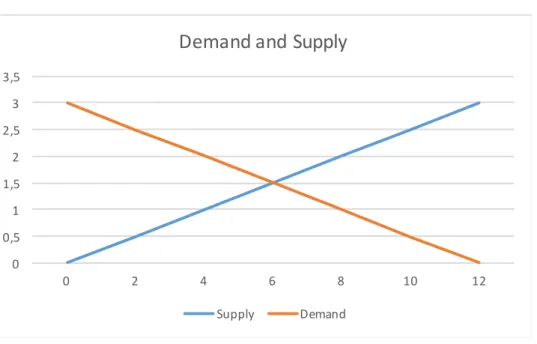
Having defined demand and supply on its own, will help explain how these forces combined help define prices. Figure 3 shows the result of putting together both demand and supply graphs.
0 0,5 1 1,5 2 2,5 3 3,5 0 2 4 6 8 10 12
Supply
SupplyFigure 3: Demand and Supply
On Figure 3 it is clearly observed that demand and supply intersect at one point which is where the price (equilibrium price) is $1, 5 and quantity (equilibrium quantity) is 6; this point is called market’s equilibrium. “At the equilibrium price, the quantity of the good that buyers are willing and able to buy exactly balances the quantity that sellers are willing and able to sell. The equilibrium price is sometimes called the market-clearing price because, at this price, everyone in the market has been satisfied: Buyers have bought all they want to buy, and sellers have sold all they want to sell.”7
When looking at the demand and supply graph presented above, everything that is above the equilibrium point implies that there is a surplus of the product/service in the market. Let’s take for example a price of $2,5, what can be observed is that for that price there will be only demand for 2 units of the product/service but on the other side there will be supply of 10 units of the product/service thus being oversupplied. At this point, given that the seller has more units of the product/service but customers are not willing to buy at this price, the seller has to respond to this surplus by lowering its prices bringing the market into equilibrium again.
On the other hand, when looking below the market’s equilibrium there is excess demand of the product/service in the market. To illustrate this point, taking a price of $0,5 will imply a demand of 10 units of the good but there will only be a supply of 2 units because it is not profitable for
7Mankiw,N.Gregory,,. (2015). Principles of macroeconomics 0 0,5 1 1,5 2 2,5 3 3,5 0 2 4 6 8 10 12
Demand and Supply
the producer to sell at this price. At this point, given that there is shortage of the product/service, the producer/seller raises prices affecting the good’s demand and coming back to market equilibrium.
Changes either on the demand or the supply side will bring new equilibriums for both price and quantity of the product/service being studied. Given this, we can infer that price changes for any good is determined by a change either on the demand or the supply side so oil shocks can be explained due to excess demand (shortages) or excess supply (surplus) of this commodity in the market.
2.1 2003-2008 Oil Price Rise and Plunge
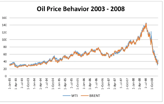
Oil prices began to raise in mid 2003 increasing consistently until 2008 when the price raised from Usd$25.25 per barrel in late April 2003, to Usd$145.31 per barrel early in July 2008 representing a 475% raise, and to later close the 2008 in Usd$44.6 per barrel representing a 69% drop in the Price versus its peak.
Figure 4: Oil Price Behavior 2003 - 2008
Source: U.S. Energy Information Administration (EIA)
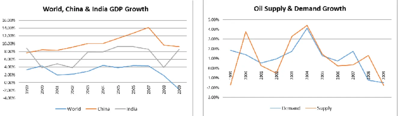
Movements in oil prices during this period are explained by an increase in the demand of the commodity driven mainly by world economic growth after the early 2000’s economic crisis. Growth was mainly driven by emerging economies such as China that grew at double digits
from 2003 until 2007; and India, which grew above 8% in nearly every year over the same period. These two countries led the world economy to grow above 4% from 2004 until 2007 as seen in Figure 5.
Figure 5: World, China & India GDP Growth / Oil Supply & Demand Growth
Source: World Bank & Organization of the Petroleum Exporting Companies (OPEC)
In this growing trend, countries tend to demand more energy to increase its output, which translates in an increase of oil demand. After the crisis oil had a positive increase in the demand growing at similar pace with oil supply until demand growth surpassed supply growth driven by a high growth in China’s an India’s economies showing one of the highest growth rates in this period. This is clearly observed in oil price behavior observed in Figure 5 were oil prices hiked most of the Usd$84.1 per barrel surge from January 1st 2006 until its peak in July 2008.
More than half of the increase in the price of oil in the 2006-2008 period was presented on the first half of 2008 were the Price hiked Usd$45.99 per barrel from the beginning of the year until July. This hike on such a short period is believed to be produced by speculators in the commodities derivatives markets but the reality is that it was driven by a series of events that affected oil supply in the first half of the year. The events are as follows: “In February 2008 Venezuela cut off oil sales to ExxonMobil during a legal battle over nationalization of the company’s properties there. Production from Iraqi oil fields, of course, had still not recovered from wartime damage, and in late March saboteurs blew up the two main oil export pipelines in the south—cutting about 300,000 barrels per day from Iraqi exports. On April 25, Nigerian union workers went out on strike, causing ExxonMobil to shut in production of 780,000 barrels per day from three fields. Two days later, on April 27, Scottish oil workers walked off the job, leading to closure of the North Forties pipeline that carries about half of the United Kingdom’s North Sea oil production. As of May 1, about 1.36 million barrels per day of Nigerian
production was shut in due to a combination of militant attacks on oil facilities, sabotage, and labor strife. At the same time, it was reported that Mexican oil exports (tenth largest in the world) had fallen sharply in April due to rapid decline in the country’s massive Cantarell oil field. On June 19, militant attacks in Nigeria caused Shell to shut in an additional 225,000 barrels per day. On June 20, just days before the price of oil reached its historic peak, Nigerian protesters blew up a pipeline that forced Chevron to shut in 125,000 barrels per day. Each of these events clearly registered in the spot market. It is not implausible to believe that, arriving in quick succession, they contributed heavily to the rapid acceleration in the spot price of oil.”8
Prices plunge in the second half of 2008 can also be explained from the demand side. After the subprime crash in 2007, the world entered in a deep recession were growth slowed down dramatically in 2008 and even presented a negative growth of -1.68% in 2009 which was translated to a dramatic reduction in world oil demand were it declined 1.22% in 2008 an 1.49% in 2009.
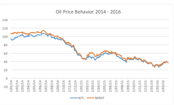
2.2 2014 Price Shock
At mid 2014 oil prices started to decrease and by early 2015 the falling prices had become dramatic having WTI price going down 76% from its peak in June 2014 to its lowest price in January 2016; for Brent prices, a similar decrease was observed were a 77% fall in the price was observed from its highest quote in June 2014 to its lowest price in February 2014. Oil prices have recovered from its lows but they are still far away form prices observed in 2014. Figure 6 shows Oil prices behavior from January 2014 until March 2016 were oil price dramatic fall starting in June 2014 ca be observed.
8Smith, J. L. (2009). The 2008 Oil Price: Markets or Mayhem?, http://www.rff.org/blog/2009/2008-oil-price-shock-markets-or-mayhem, Accessed August 20,2016.
Figure 6: Oil Price Behavior 2014 - 2016
Source: U.S. Energy Information Administration (EIA)
2014 oil price shock was mainly due to an unexpected increase in the supply, main factors that affected world oil supply are as follows:
United States Shale Oil Production: “Since 2011, U.S. shale oil production has persistently surprised on the upside, by some 0.9 million barrels per day (mb/d, about 1 percent of global supply) in 2014.”9
OPEC decision not to cut oil production: In November 2014 OPEC meeting, there was no agreement in cutting current production levels of 30 mb/d in order to control prices as they have previously done when prices plunged. Its most important member, Saudi Arabia who is usually the one member that can swing prices by shifting its production refused to reduce its production as a strategy to gain market share.
Expected supply disruptions due to geopolitical incidents: Oil world supply was expected to be reduced due to internal conflicts in Libya, Iraq ISIS advance and sanctions on Russia after their military invasion in Ukraine but supply was not reduced, given that in Libya, “despite the internal conflict, production recovered by 0.5 million
9 Understanding the Plunge in Oil Prices: Sources and Implications -20 0 20 40 60 80 100 120 140 2 /0 1 /1 4 2 /0 2 /1 4 2 /0 3 /1 4 2 /0 4 /1 4 2 /0 5 /1 4 2 /0 6 /1 4 2 /0 7 /1 4 2 /0 8 /1 4 2 /0 9 /1 4 2 /1 0 /1 4 2 /1 1 /1 4 2 /1 2 /1 4 2 /0 1 /1 5 2 /0 2 /1 5 2 /0 3 /1 5 2 /0 4 /1 5 2 /0 5 /1 5 2 /0 6 /1 5 2 /0 7 /1 5 2 /0 8 /1 5 2 /0 9 /1 5 2 /1 0 /1 5 2 /1 1 /1 5 2 /1 2 /1 5 2 /0 1 /1 6 2 /0 2 /1 6 2 /0 3 /1 6
Oil Price Behavior 2014 - 2016
barrels per day (about 1⁄2 percent of global production) in the third quarter of 2014.”10 In Iraq, ISIS advance was stopped on the last months of 2014 and sanctions on Russia didn’t had the effects on oil production that the markets were expecting.
On the other hand, there were also other implications that affected the demand for oil also affecting the price of this commodity:
Global Growth: The world is still recovering from the 2007 financial crisis and recovery has been slower than expected. Additionally, China who was driving world economic growth over the last years started to decelerate its growth growing 6.9% in 2015 when it was growing at double digits before the world financial crisis. World’s growth has slowed down as a consequence of the crisis and China’s deceleration; it was growing over 4% before the crisis and has decelerated to a 2.5% growth in 2015. World Bank is expecting World growth to be of 2.4% in 2016 and will raise until 3% in 2018 while China’s growth is expected to continue to drop were a 6.7% growth is expected in 2016 and 6.3% growth for 2018. Looking at these projections, oil prices may seem to be expected to be maintained low in the following years because as explained before if the world economy’s growth does not increase, energy demand will not raise and as a consequence, oil prices will not raise.
USD currency appreciation: US dollar appreciated more than 10% on the second half of 2014 against other major currencies in the world affecting oil demand given that this commodity is traded in US currency; US revaluation erodes other countries’ purchasing power thus making it more expensive to buy oil. Estimates indicate that “a 10 percent appreciation is associated with a decline of about 10 percent in the oil price, whereas the low estimates suggest 3 percent or less.”11
10Understanding the Plunge in Oil Prices: Sources and Implications 11Understanding the Plunge in Oil Prices: Sources and Implications
3 Colombia Oil Market Overview
Oil industry in Colombia has over 100 years of history, its origins dates back to 1905 when the “Barco” (October 1905) and “De Mares” (November) concessions were signed. Ever since the industry started, Colombia has received capital inflows for exploration and exploitation of crude. Colombia’s largest oil company is Ecopetrol (Empresa Colombiana de Petróleos) which is state owned and was founded in 1951.
Colombia´s oil production has been increasing over the past years, and currently is producing over 1 million barrels, almost doubling its production in the last decade. Increase in oil production is a result of regulatory reforms made in 2003 by President Uribe making more international firms to invest in Colombia by providing a friendlier environment for investors permitting foreign companies to completely own oil ventures in the country competing directly with the state owned Ecopetrol.
3.1 Colombia Oil Production
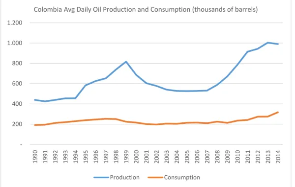
Oil production was stagnated at around 500 thousand barrels per day but on 2008, oil production started to grow at an accelerated rate driven by the increase in exploration. This increase can be explained because with 2003 reforms, more companies were able to form part of the exploitation and exploration phases that in the past were only performed by large corporations. With the mentioned reform, even service companies entered in the exploration and exploitation phase of the oil supply chain.
On the other hand, oil consumption in the country has remained relatively stable for the past 25 years meaning that Colombia’s oil exporting capacity has increased since 2008. Both bevaviours (daily production and consumption) can be observed in Figure 7 below.
Figure 7: Colombia Avg Daily Oil Production and Consumption (thousands of barrels)
Source: UPME (Unidad de Planeación Minero Energética)
It is important to highlight that the hike in oil production is not due to an increase in finding new oil sources but is attributed to wells discovered years ago. “According to UPME, nearly 90% of current production comes from oil fields discovered more than two decades ago and from the 1,220 millions of barrels incorporated to the reserves from 2003 to 2008, 80% has been due to revaluation of existent fields and the other 20% by new discoveries.”12 Part of the increase in oil production comes from heavy oil that was possible given the high prices of the commodity; otherwise, it would have not been profitable to invest in extracting this oil.
3.2 Oil Exports
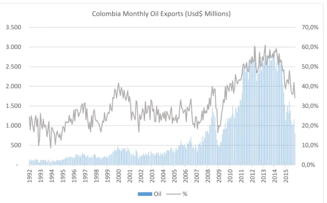
As seen before, Colombia produces more oil than what the country consumes, so in this order of ideas, Colombia is a net oil exporter. The rapid growth in oil production in the country is traduced in an increase of oil exports in the last 6 years reaching its peak in 2013 with over Usd$32 Billion accounting for 55% of the country’s total exports as shown in Figure 8.
12 Toro, J., Garavito, A., López, D. C., and Montes, E., 2015. El choque petrolero y sus implicaciones en la economía Colombiana. Borradores de Economía Núm. 906. Bogotá: Banco de la República.
200 400 600 800 1.000 1.200 199 0 199 1 199 2 199 3 199 4 199 5 199 6 199 7 19 98 199 9 200 0 200 1 200 2 200 3 200 4 200 5 200 6 200 7 200 8 200 9 201 0 201 1 201 2 201 3 201 4
Colombia Avg Daily Oil Production and Consumption (thousands of barrels)
Figure 8: Colombia Monthly Oil Exports (Usd$ Millions)
Source: DANE (Departamento Administrativo Nacional de Estadísticas)
Figure 8 shows Colombia’s monthly oil exports (left axis) and the percentage it represents from monthly exports (right axis). It is very clear that oil exports have raised sharply after 2008 were the country’s production started to increase as explained before. It is important to notice that reduction in exports that started at the end of 2014 is not entirely explained by a decrease in the exported amounts, exported amounts have decreased only in 3% falling from 44.7 million metric tons exported accumulated from January to November 2014 to 43.2 million metric tons exported in the same period in 2015, so it is clear that the decline in exports is mainly explained by a decline in international oil prices.
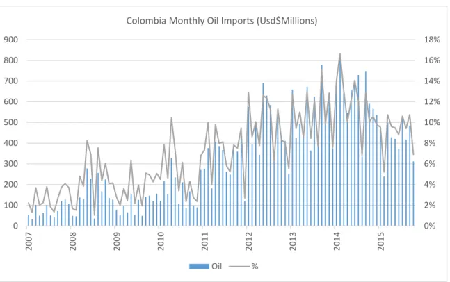
3.3 Oil Imports
Even though Colombia produces more oil than the one it consumes, there are certain oil derivative products that the country has to import mainly because the oil produced in Colombia is heavy and sour and the country doesn’t have enough refineries to process its type of crude to comply with local demand. Oil imports only account for 9% of total imports accumulated in the first 10 months of 2015 vs the 41% that crude oil exports represent for the same period as observed in Figure 9. 0,0% 10,0% 20,0% 30,0% 40,0% 50,0% 60,0% 70,0% 500 1.000 1.500 2.000 2.500 3.000 3.500 1992 1993 1994 1995 1996 1997 1998 1999 2000 2001 2002 2003 2004 2005 2006 2007 2008 2009 2010 2011 2012 2013 2014 2015 Colombia Monthly Oil Exports (Usd$ Millions)
Figure 9: Colombia Monthly Oil Imports (Usd$ Millions)
Source: DANE (Departamento Administrativo Nacional de Estadísticas)
As it happened with exports, imports have fallen on the last months explained by the decline i international oil prices.
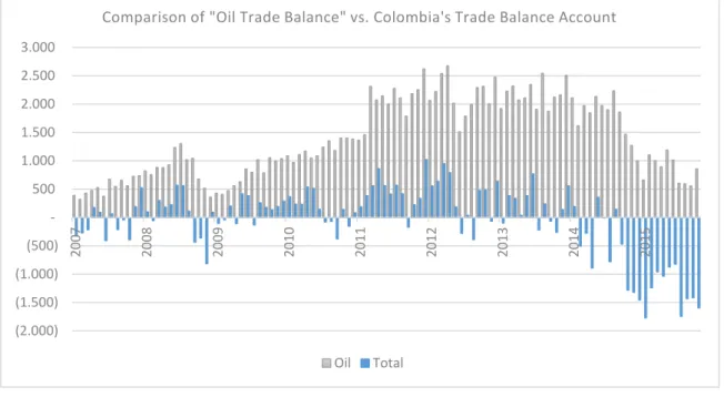
3.4 Trade Balance
Taking into account the information provided for both imports and exports for oil, we can confirm what was stated before on this paper: Colombia is a net oil exporter. If a separate Trade Balance (difference between exports and imports) is run for only this part of the economy, the “oil trade balance” for Colombia will be positive wera an increase will be observed between 2008 to 2014 and a decline will be seen on 2015 due to lower oil prices.
Figure 10 compares “oil trade balance” with the country’s total trade balance, and from the graph, it is obvious that if Colombia did not have oil surplus, trade balance would be much more negative than it currently stands.
0% 2% 4% 6% 8% 10% 12% 14% 16% 18% 0 100 200 300 400 500 600 700 800 900 2007 2008 2009 2010 2011 2012 2013 2014 2015
Colombia Monthly Oil Imports (Usd$Millions)
Figure 10: Comparison of “Oil Trade Balance” vs. Colombia’s Trade Balance Account
Source: DANE (Departamento Administrativo Nacional de Estadísticas)
Looking at Figure 10, it is observed what was just described above; if Colombia oil exports diminish or even disappear, there will be a huge impact on the country’s trade balance that will have many macroeconomic consequences in the country starting by currency devaluation, followed by higher inflation due to devaluation pass-through to Consumer Price Index given that the country is net importer; then followed by a restrictive monetary policy were the central bank will have to raise interest rates to fight raising inflation; and finally comes growth slowdown because internal consumption will deteriorate due to higher interest rates.
(2.000) (1.500) (1.000) (500) 500 1.000 1.500 2.000 2.500 3.000 2007 2008 2009 2010 2011 2012 2013 2014 2015
Comparison of "Oil Trade Balance" vs. Colombia's Trade Balance Account
4 Importance of Oil Prices in Colombian Economy
As mentioned above, Oil price volatility affects many aspects in the Colombian economy such as the country exchange rate, inflation (measured as Consumer Price Index), current account and last but not least important its Gross Domestic Product. In this chapter, we will show tendencies of how these indicators are being affected by oil prices.
4.1 Current Account
Oil prices have a direct effect on Colombia’s current account from the trade balance standpoint as mentioned above and also from foreign direct investment (FDI) inflows to the country. When oil prices are low, normally what happens is that there are less capital inflows to the country for oil exploitation purposes because it becomes non-profitable to extract oil. Oil inflows have averaged over 33% of FDI inflows in the last decade averaging nearly Usd$4 billion dollars entering the country per year.
Figure 11: Foreign Direct Investment (FDI) and Oil Prices
Source: Banco de la República de Colombia and U.S. Energy Information Administration (EIA)
Figure 11 shows that there is a direct relationship of oil prices and FDI figures in the Colombian case. Oil related FDI started to surge as soon as oil prices started to raise between the years 2005 and 2006 were WTI (annual average) prices were above Usd$50 per barrel. The upward tendencies (of both WTI and Oil FDI) continued until the period between 2011 and 2014 were
0 20 40 60 80 100 120 -2.000 0 2.000 4.000 6.000 8.000 10.000 12.000 14.000 16.000 18.000
FDI and Oil Prices
oil prices averaged nearly Usd$100; for 2015 a decrease in both oil price and Oil FDI was seen reaffirming that they have a direct relationship that is confirmed when applying a simple correlation analysis of Oil price vs. Oil FDI giving as a result a correlation index of 0.93
4.2 Exchange Rate
The effects on current account has a direct impact on Colombia´s currency (Peso) given that the country has a flexible exchange policy were the Peso fluctuates freely according to the offer and demand principles; when offer increases prices decline and when offer declines, prices increase. Applying this principle to the exchange rate, as dollar inflows increase exchange rate declines and the opposite happens when dollar inflows are reduced. Given that a direct relationship between oil current account and the price of oil was described above, an inverse relationship between oil prices and exchange rate represented as the TRM13 (Tasa Representativa del Mercado).
Figure 12: TRM vs. WTI and Brent Prices
Source: Banco de la República de Colombia and U.S. Energy Information Administration (EIA)
13Is the daily market exchange rate, it is the amount of colombian pesos that must be paid for 1 US dollar. It is calculated based on buy and sell spot transaction between financial intermediaries in the Colombian exchange market that are fullfilled the same day the transaction was negotiated.
0 20 40 60 80 100 120 140 160 $ 0,00 $ 500,00 $ 1.000,00 $ 1.500,00 $ 2.000,00 $ 2.500,00 $ 3.000,00 $ 3.500,00 $ 4.000,00
TRM vs. WTI and Brent
On Figure 12 daily oil prices (WTI and Brent) are compared vs. daily TRM, were a clear inverse relationship between the variables is observed. This behavior can be explained because when oil prices are down, there are going to be less US dollars entering the Colombian economy affecting the offer side thus increasing the number of pesos to be paid for the US currency. On the other side, when oil price rises, US dollar inflows are expected to increase thus incrementing the offer of the currency in the country and lowering its price. When making a simple correlation analysis of TRM vs WTI and Brent oil prices for this daily series starting 2001, we obtain -0,73 and -0.74 correlation coefficient for WTI and Brent prices correspondingly confirming there is a high inverse relationship between the variables mentioned above.
4.3 Oil Production
Another observable consequence of a reduction in FDI is stagnation in oil production in the country. If no resources are being allocated to find new oil sources in the country, production will be affected, at the beginning, production will stagnate, but if FDI doesn´t recover, a reduction in production will be seen in the future, because oil resources in the country start to diminish and become scarce.
Figure 13: Colombian Oil Production vs. Oil Prices
Source: UPME (Unidad de Planeación Minero Energética) and U.S. Energy Information Administration (EIA) 0 200 400 600 800 1.000 1.200 0,0 20,0 40,0 60,0 80,0 100,0 120,0 140,0 160,0 01/jan /00 01/o u t/00 01/ju l/01 01/ab r/02 01/jan /03 01 /o u t/0 3 01/ju l/04 01/ab r/05 01/jan /06 01/o u t/06 01/ju l/07 01 /ab r/08 01/jan /09 01/o u t/09 01/ju l/10 01/ab r/11 01/jan /12 01/o u t/12 01/ju l/13 01/ab r/14 01/jan /15 01/o u t/15
Colombian Oil Production Vs Oil Prices
When comparing both WTI and Brent prices (left index) vs Colombian oil production (right index in thousands of barrels per day) on Figure 13, we observe that as oil prices went up in 2009, there was an increase of oil production from 600,00 barrels a day to over 1,000,000 barrels per day in late 2014 and beginning of 2015 were production stabilized for a while until it started to fall in 2016 were production has constantly been below this figure. It can be inferred that as FDI destined to oil activities is reduced, oil production stabilizes for a while and can deter if investment doesn´t raise again.
4.4 Consumer Price Index (CPI)
Consumer price index (CPI) is an indicator that measures the change of prices of a basket of goods and services that is made to represent the consumption of Colombian households. This is an important measurement because it measures the increase of the costs of living in the country on a yearly basis. Given that Colombia is a net importer, it is assumed that it imports goods for local consumption, so if the currency depreciates, we expect the indicator to go up because imported goods will become more expensive for retailers and the increment will be passed to the final consumer thus incrementing the cost of life; if the currency appreciates, the opposite is expected to happen, prices go down and consumer price index will decrease as the lower prices are transferred to consumers.
Figure 14: WTI Prices vs. CPI Yearly Change
0 20 40 60 80 100 120 140 160 0, 2, 4, 6, 8, 10, 12, jan /00 se t/00 mai/01 jan /02 se t/02 mai/03 jan /04 se t/04 mai/05 jan /06 se t/06 mai/07 jan /08 se t/08 mai/09 jan /10 se t/10 mai/11 jan /12 se t/12 mai/13 jan /14 se t/14 mai/15 jan /16
WTI Vs CPI YOY Change
Source: Departamento Nacional de Estadística (DANE) and U.S. Energy Information Administration (EIA)
On Figure 14 we see there is an inverse relationship of oil prices (WTI on the right axis) with CPI and Core CPI year on year confirming what was explained just above. When looking at the correlation coefficients core CPI shows a higher inverse relationship than total CPI (-0.75 for Core vs. -0.70 for Total). This phenomenon can be explained mainly because total CPI includes food inflation that is very volatile and its variation depend on weather changes and other exogenous factors such as strikes.
4.5 Gross Domestic Product (GDP)
As defined by Callen at the International Monetary Fund (IMF) “GDP measures the monetary value of final goods and services—that is, those that are bought by the final user—produced in a country in a given period of time (say a quarter or a year). It counts all of the output generated within the borders of a country. GDP is composed of goods and services produced for sale in the market and also include some nonmarket production, such as defense or education services provided by the government.”14 Taking this definition as a base, GDP measures a country’s performance for a given period of time.
Colombia’s economy has been growing faster than the world economy over the last years mainly because since the financial crisis in 2007, developed economies entered into recession and after recovery, their growth has been pretty low. Colombia’s performance has been boosted in part by oil that increased its participation in the country’s income from 7.4% in 2002 to 19.5% in 2013. After 2013, oil participation from the nation’s income started to decrease, in 2013 oil income accounted for 3.3% of total GDP, in 2014 it went down to 2,6%, it went further down in 2015 to 1.1% and for 2016 it is expected to be negative in -0.8% of GDP. Oil income outlook for Colombia is not very promising, Minister of Finance is expecting oil income in the long term to remain in 0.4% of GDP, which is far below the figures observed when oil prices were up.
14 Callen, T., 2012. Gross Domestic Product: An Economy’s All. Finance & Development, http://www.imf.org/external/pubs/ft/fandd/basics/gdp.htm , accessed August 07, 2016.
Figure 15: GDP Growth vs. Oil Prices
Source: Banco de la República de Colombia (Banrep) and U.S. Energy Information Administration (EIA)
When comparing Colombia’s GDP growth (left axis) with WTI and Brent oil prices (right axis) it can be observed that there is a clear relationship between oil prices and the country’s overall performance. Even though correlations on this period of time is not so high (0.42 for WTI and 0.41 for Brent) the graph indicates that economy’s growth follows oil prices. Low correlation can be because there are other factors in the country different form oil prices that affect its performance and also because it may be that the effects of a decline/rise in prices is not reflected in the same quarter as when it occurred but can have a lag between the occurrence of the oil shock and its effects on the economy.
20 40 60 80 100 120 140 0,00 1,00 2,00 3,00 4,00 5,00 6,00 7,00 8,00 9,00 mar/01 ou t/01 mai/02 dez/02 ju l/03 fev/04 set/04 abr/ 05 n o v/05 ju n /06 jan /07 ag o /07 mar/08 ou t/08 mai/09 dez/09 ju l/10 fev/11 set/11 abr/ 12 n o v/12 ju n /13 jan /14 ag o /14 mar/15 ou t/15
GDP Growth Vs. Oil Prices
5 Literature Review
Many papers have been written about the effects of oil in country’s or region’s economies all over the world, but little literature can be found about the effects of oil in Colombia. There is a paper published on 2009 by the ex-ministry of finance and now president of Ecopetrol Juan Camilo Echeverry called Oil In Colombia: History, Regulation and Macroeconomic Impact; the paper presents a history of oil in the country, then explains changes in the regulations that has permitted an increase of capital inflows for oil exploitation; finally the author explains the events of the short oil boom in the nineties and concludes that Colombia’s performance at the end on the nineties is attributed to this boom because the country entered in a phase of fiscal relaxation driven mainly by increasing its expenses due to the oil boom which later was traduced in more debt for the country. Finally, the author recommends that if there is a future oil boom, “is to pass a law, before any important discoveries are made, defining the use of increased state resources. This is the only way a pillage policy can be avoided once a bounty treasure is at sight.” 15
Since there is not too much research regarding Colombia, a study from Hesary, Yoshino, Abdoli and Farzinvash published in 2013 where they evaluated “the impact of oil price shocks on oil producing and consuming economies”16. They conducted a quantitative research study where they compared the effects of a positive oil price shock vs. the GDP of each of the countries analyzed. The result was that there was a positive relation between raising oil prices and exporters (Iran and Russia in the study they conducted) GDP.
Prices move based on the two main market forces that are supply and demand. If there is a higher demand of a good and the production of this good remains constant (supply side) the price is supposed to rise, on the other hand, when the supply is higher than the demand, prices fall. In oil prices this theory is being questioned by Hesary and Yoshino in their 2014 paper “Monetary policies and oil price determination: an empirical analysis”. The authors explain that expansionary monetary policies have induced an increase in oil demand that led to a slower economic growth. They concluded that “Aggressive monetary policy stimulates oil
15Echeverry, J.C., Navas, J., Navas, V., and Gómez, M.P., 2009. Oil in Colombia: History, Regulation and Macroeconomic Impact. Documentos CEDE. 2009-10. Bogotá: Ediciones Uniandes.
16Hesary, T., Yoshino, N., Abdoli, J., and Farzinvash, A., 2013. An Estimation of the Impact of Oil Shocks on Crude Oil Exporting Economies and Their Trade Partners. Frontiers of Economic in China 2013, 8(4).
demand, while supply is inelastic to interest rates.”17
17Hesary, T., and Yoshino, N., 2014. Monetary Policies and Oil Price Determination: An Empirical Analysis.
6 Model Description
In this section, we analyze the behavior of the Colombian economy with a Vector Auto Regression (VAR). VARs have been used since the 1980s to summarize the dynamics of an economy by combining series associated with economic activity, prices, interest rates as well as external indicators. In the macroeconomic literature (Juselius, 2006), as long as the series share a common trend, what is traditionally known in the economics literature as cointegration, it is possible to use the variables without differentiating them. In this case, we should refer to this model as a cointegrated VAR. The description of the variables used will be adressed in section 6.2.
6.1 Vector Autoregression (VAR) Definition
In order to determine the impact of an oil shock Price in Colombia’s economy a vector autoregression (VAR (p)) model was estimated using the variables described in section 6.2. The model can be described in its general form as:
𝑦𝑡 = c + ∑ 𝐴𝑖𝑦𝑡−𝑖+ 𝑢𝑡 𝑝
𝑖=1
Where:
𝑐 is a 6x1 vector constant;
𝒚𝒕 is a 6x1 vector that includes the variables that make up the system at time t; 𝑨𝒊 corresponds to the ith 6x6 parameter matrix; and
𝒖𝒕 is a 6x1 vector error term.
Vector 𝒚𝒕 can be described more specifically in the following form: 𝑦𝑡= (𝑖𝑠𝑒𝑡 𝑐𝑝𝑖𝑡 𝑟𝑒𝑝𝑜𝑡 𝑢𝑠𝑑𝑐𝑜𝑝𝑡 𝑡𝑏𝑡 𝑤𝑡𝑖𝑡)′ Where:
𝒊𝒔𝒆𝒕 is the natural logarithm of the monthly activity index (ISE) for Colombia; 𝒄𝒑𝒊𝒕 is the natural logarithm of consumer price index;
𝒓𝒆𝒑𝒐𝒕 is the Central Bank’s policy rate;
𝒖𝒔𝒅𝒄𝒐𝒑𝒕 is the natural logarithm of the exchange rate in terms of Colombian Pesos per US Dollar;
𝒕𝒃𝒕 is the country’s trade balance, in US Dollar terms; and
𝒘𝒕𝒊𝒕 is the natural logarithm of the average monthly market price for one-month West Texas Intermediate (WTI) oil futures.
In the model above, p corresponds to the number of lags included in the model. In order to determine the number of lags for our estimation, lag selection criteria recommended running the VAR model with one, two and four lags, depending on the criteria used. With the three models at hand, information criteria were used to select the final VAR (4) model. In addition, the fact that the model was estimated using monthly data allows a higher lag count without compromising too many degrees of freedom, and thus captures more variability in the autoregressive process.
An impulse response function on the variables was analyzed to interpret the effects of oil prices in main Colombian indicators. The variable shocked in this model is the oil price (𝒘𝒕𝒊𝒕) and based on this shock the timing and magnitude of an oil price shock in the Colombian economy will be interpreted.
6.2 Variables Description
Monthly Activity Index: It is measured through ISE (Indicador de Seguimiento de la Economía) for its acronym in Spanish is an indicator that was created to provide a measurement of the economic activity in the short term. This index is published on a monthly basis and has a lag of maximum two months in the data. It is calculated using a methodology adjusted to the one of the quarterly national accounts and is composed by a set of heterogeneous indicators that are representative of each economic activity. This index cannot be assumed to be a monthly Gross Domestic Product (GDP) because it doesn’t measure the aggregate value generated by the nation in each time interval and it doesn’t include the taxes associated to each economic activity. This indicator is published by Departamento Administrativo Nacional de Estadísticas (DANE).
This indicator is used in the model because it measures the performance of the country´s economy and by shocking the WTI prices it will help to illustrate how the economy is affected by oil prices. This indicator was used instead of the GDP because it is published on a monthly basis rather than quarterly as is the case of GDP; having monthly information gives us more data points to include in the model increasing the degrees of freedom in case the data needs to be lagged. Additionally, recently it was proved that ISE’s behavior resembles GDP, Citi Research found that “that the indicator provides reliable information to track activity growth
through a quarter before GDP data for that quarter is released, thus making the ISE a good up-to-date source to track activity and gauge GDP evolution.”18
Inflation: Inflation in Colombia is measured through IPC (Índice de Precios al Consumidor) for its acronym in Spanish but is the exact translation to CPI (Consumer Price Index). CPI measures the evolution of the average cost of a basket of goods and services in time. The percentage difference of the price of this basket in one point in time vs. another is the CPI for that given period. Colombia announces inflation figures on a monthly basis and they publish monthly inflation, year to date inflation and yearly inflation. Inflation is published by Departamento Administrativo Nacional de Estadística (DANE).
This indicator is important to the model because it helps measure the change in the cost of living in the country represented by the prices of goods and services which are set by the forces of demand and supply.
Central Bank Policy Rate: Is the intervention rate set by the Colombian Central Bank (CB) board of governors on a monthly basis. This rate is the main instrument the bank has to regulate the monetary policy of the country by affecting the amount of cash outstanding in the economy. If rates go up the CB adopts a contractionary policy where they wish to reduce the demand for money by making it more expensive for people to access credit which in consequence affects the country’s economic growth; if rates are lowered by CB, they are adopting an expansionary policy making the money more inexpensive thus facilitating the access to credit and increasing the monetary base, as a consequence of this action economic growth is expected. This rate is the minimum rate at which CB lends money to banks (via Repo auctions) and the maximum rate at which the CB pays for resources received from banks. In the Colombian market it is commonly called the repo rate and is published by Banco de la República de Colombia (Banrep – Colombia’s CB) on a monthly basis after the board of governors meeting.
This variable is included in the model because it helps to illustrate whether if the Central Bank takes actions to promote/discourage economic growth to offset the outcomes of an oil price shock by applying an expansionary or contractionary monetary policy.
18Citibank Research Colombia, The ISE Monthly Activity Indicator and Slowing Activity Growth, September 13, 2016
Trade Balance: It is the difference between the country’s exports and its imports. It is the largest component of the balance of payments. The balance of payments as defined by Colombia’s Central Bank is an “accountancy record of all the economical transactions of the country's residents with the rest of the world during a given period of time, generally a year. In other words, it shows total payments made abroad, and the total amount received from abroad. It records both the flow of real resources (goods and services) and the flow of financial resources (the movement of capital).”19 Trade balance information is published by Colombia’s Central Bank (Banco de la República de Colombia) on a monthly basis while balance of payments is published on a quarterly basis.
This information is important because as was previously discussed, Colombia is a net oil exporter and ever since 2004 oil has been gaining importance in the export figures of the country.
USDCOP Exchange Rate: It corresponds to the number of Colombian Pesos (Cop) someone has to pay to buy one United States Dollar (Usd). In Colombia the official exchange rate for a given day is called TRM (Tasa Representativa del Mercado) for its Spanish acronym. This rate is calculated based on buy and sell spot transaction between financial intermediaries in the Colombian exchange market that are fulfilled the same day the transaction was negotiated. This rate is calculated and published by the Finance Superintendence (Superintendencia Financiera de Colombia) on a daily basis based on the FX operations made on the day of the publication. The exchange rate is the price at which one currency is expressed in terms of another nation’s currency and many currencies are quoted against the US dollar as is the case for Colombia. The exchange rate is influenced by many factors such as political stability, trade balance, inflation and interest rates just to name a few. Given that the exchange rate captures a wide range of factors, it is important to include it in the model to help determine how the oil prices affect the exchange rate.
WTI Price: As defined by U. S. Energy Information Administration (EIA), West Texas Intermediate (WTI) is “A crude stream produced in Texas and southern Oklahoma which serves as a reference or "marker" for pricing a number of other crude streams and which is traded in the domestic spot market at Cushing, Oklahoma.”20 The Price that will be used for this variable
19 http://www.banrep.gov.co/en/node/23604
used will be the monthly Cushing, OK WTI spot Price FOB; information is published by numerous sources but for this model the information was accessed through the EIA.
The model will be feed with monthly data for each of the before mentioned variables starting January 2003 until March 2016. Fort Monthly Activity Index monthly seasonally adjusted published data will be used and the source of the information will be DIAN; for Inflation CPI (IPC in Spanish) published data will be used and the source will be DIAN; for Central Bank Policy Rate the rate that will be used will be that rate that applied on month end for each of the observations, data will be obtained from Banrep, Colombia’s CB; Trade Balance figures used will be the official monthly figures published by Banrep; USDCOP Exchange Rate month end exchange rate will be used and the source of the information is Superintendencia Financiera de Colombia; and for WTI Prices data used will be the average monthly Cushing, OK WTI spot Price FOB and the source of the information will be EIA.
Data was chose to start January 2003 mainly because it is the year when Colombia’s Central bank started to set inflation targets by ranges and also in 2003 was when oil prices started to raise after the early 2000’s crisis in the world as explained earlier. This information will enable the model to incorporate two oil prices crash, the one in 2008 after the world financial crisis and the latest plunge in prices seen in 2014 and still endures. No information before the 2000’s was included in this data mainly because Colombian monetary and exchange policies presented a shift between 1999 and late 2000; in 1999 Colombian CB changed the exchange policy were it used to have an exchange rate band and on September 25th 1999 CB decided to eliminate this mechanism and let the exchange rate freely flow determined by the forces of supply and demand; regarding monetary policy, on October 2000 CB adopted an inflation target monetary policy but it is not fully consolidated until 2003 were long term inflation target ranges were set oscillating from 2% to 4% being 3% the target point.
6.3 Determining the Number of Lags in the Model
In order to determine the number of lags to be applied to the VAR model, a series of tests were run. The tests performed to determine the lag length are:
LR: sequential modified LR test statistic (each test at 5% level) FPE: Final prediction error
AIC: Akaike information criterion SC: Schwarz information criterion
HQ: Hannan-Quinn information criterion The results are resumed in the following table:
Table 1: Lag Tests Results
VAR Lag Order Selection Criteria
Endogenous variables: LOGISE INF REPO LOG(USDCOP) X LOG(WTI) Exogenous variables: C
Date: 09/30/16 Time: 21:12 Sample: 2000M01 2018M12 Included observations: 175
Lag LR FPE AIC SC HQ
0 NA 6,467765 18,89409 19,0026 18,93811 1 2633,501 1,52E-06 3,629923 4.389471* 3.938017* 2 100,691 1.23e-06* 3,419802 4,830392 3,991977 3 50,72268 1,35E-06 3,506085 5,567717 4,342342 4 75.37180* 1,24E-06 3.415035* 6,127709 4,515373 5 33,95283 1,49E-06 3,59068 6,954395 4,955099 6 34,03146 1,79E-06 3,755504 7,770261 5,384004 7 34,55074 2,13E-06 3,905184 8,570983 5,797765 8 39,48063 2,42E-06 4,003275 9,320115 6,159937
* indicates lag order selected by the criterion
Two criteria were met determining that the model should be run with 1 or 4 lags and only 1 recommended to use 2 lags. Given that it was discarded to run the model with 2 lags and the decision is to be made between 1 or 4 lags.
In order to determine the lags, two criteria were taken into account: first of all, we understand that a shock in oil prices not necessarily has an immediate effect on the country’s economy, normally the effects are seen some months after the prices fall, mainly because part of the production is normally sold in advance in the derivatives market or could also be hedged in advance thus not transferring the loss in price immediately.
Secondly, even though the above argument is true, it was decided to have a statistical reason to decide between VAR (1) and VAR (4) models. The models were run and the R-squared of both
models were run for all of the variables giving as a result that VAR (4) had a higher R-square in all of the variables as observed in the following table:
Table 2: R-Squared For Var(4) and Var(1) Models:
LOGISE INF REPO LOG(USDCOP) X LOG(WTI)
VAR(4) 0.9989 0.8995 0.9888 0.9591 0.7178 0.9808 VAR(1) 0.9987 0.8814 0.9845 0.9532 0.6674 0.9745
7 Results:
7.1 Descriptive Statistics:
Correlation and covariance analysis were run between all the variables to see how each variable of the model behaves when compared to the other variables in the model. As a result, it can be concluded from all the variables the following:
log (ise): This variable is negatively related to the rest of the variables except with log(wti)
where it has a positive relation. Correlations are relatively low, so it can be inferred that there is not a strong positive or negative relationship with the other variables.
cpi: It has a positive relationship with repo, and log(usdcop) and a negative one with the rest
of the variables. The only strong relationship it has is with repo having a correlation index of 0.82 meaning that these two variables will behave very similar.
repo: It has a positive relationship with cpi, log(usdcop) and tb and negative relationship with
the other variables. As mentioned before, it has a strong positive relationship with cpi.
log(usdcop): This variable has a positive relationship with cpi and repo and negative
relationship with the remaining variables. This variable has a strong negative relationship with
log(wti) meaning that when oil prices rise, this variable decreases its value in almost the same
magnitude but on the opposite direction.
tb: Trade balance has a positive relationship with repo and log(wti) and negative relationship
with the remaining variables. This variable has no strong positive or negative relationships with other variables in the model.
log(wti): Has a positive relationship with log(ise) and tb and negative relationship with the
remaining variables and has a strong negative relationship with log(usdcop) as mentioned before.
Table 3: Covariance and Correlation Analysis of Variables in the Model:
Additional to the covariance analysis, other set of statistics were run and are resumed in the following table:
Table 4: Other Descriptive Statistics:
Regarding this set of results, it can be said that all variables except tb are fairly symmetrical, while tb shows that the series is not symmetrical. On the other hand, when looking at the kurtosis results it can be observed that the only variable that is peaked against the normal is the trade balance (tb), the other variables remain flat against the normal distribution.
7.2 Unit Root and Cointegration Tests
Unit root test using the Augmented Dickey-Fuller test was performed to all the variables and the Null Hypothesis was accepted in all of the variables except in the repo variable where the Hypothesis was rejected. This means that repo series is a stationary variable while the rest of the data series are not stationary. Results of the tests can be observed in the following table:
Covariance log(ise) cpi repo log(usdcop) tb log(wti) Correlation log(ise) cpi repo log(usdcop) tb log(wti) log(ise) 0.04 log(ise) 1.00 cpi (0.24) 3.81 cpi (0.63) 1.00 repo (0.26) 3.67 5.26 repo (0.60) 0.82 1.00 log(usdcop) (0.01) 0.20 0.10 0.03 log(usdcop) (0.40) 0.63 0.27 1.00 tb (32.12) (154.15) 37.25 (40.16) 260,719.60 tb (0.33) (0.15) 0.03 (0.48) 1.00 log(wti) 0.07 (0.66) (0.46) (0.06) 57.88 0.24 log(wti) 0.70 (0.70) (0.41) (0.78) 0.23 1.00
log(ise) cpi repo log(usdcop) tb log(wti) Mean 4.75 4.86 6.12 7.70 (46.40) 4.07 Median 4.76 4.94 6.00 7.72 44.00 4.16 Maximum 5.06 8.70 12.00 8.10 1,022.00 4.90 Minimum 4.43 1.77 3.00 7.46 (1,770.00) 2.97 Std. Dev. 0.19 1.96 2.30 0.16 512.01 0.49 Skewness (0.07) 0.14 0.59 0.41 (1.43) (0.45) Kurtosis 1.77 1.93 2.53 2.16 5.39 1.98
Table 5: Unit Root Test Results
In order for the VAR model to work, the system needs to be cointegrated, in order to determine that, Johansen Cointegration tests were run (Trace statistics and maximum eigenvalue statistics) with the results being resumed in the following table:
log(ise) cpi
Null Hypothesis: LOGISE has a unit root Null Hypothesis: INF has a unit root
Exogenous: Constant Exogenous: Constant
Lag Length: 1 (Automatic - based on SIC, maxlag=14) Lag Length: 1 (Automatic - based on SIC, maxlag=13)
t-Statistic Prob.* t-Statistic Prob.*
Augmented Dickey-Fuller test statistic 0.48988 0.986 Augmented Dickey-Fuller test statistic -1.90479 0.3296 Test critical values: 1% level -3.46428 Test critical values: 1% level -3.46658
5% level -2.87636 5% level -2.87736
10% level -2.57475 10% level -2.57528
*MacKinnon (1996) one-sided p-values. *MacKinnon (1996) one-sided p-values.
repo log(usdcop)
Null Hypothesis: REPO has a unit root Null Hypothesis: LOGUSDCOP has a unit root
Exogenous: Constant Exogenous: Constant
Lag Length: 3 (Automatic - based on SIC, maxlag=14) Lag Length: 0 (Automatic - based on SIC, maxlag=14)
t-Statistic Prob.* t-Statistic Prob.*
Augmented Dickey-Fuller test statistic -2.99191 0.0374 Augmented Dickey-Fuller test statistic -1.07678 0.7248 Test critical values: 1% level -3.46464 Test critical values: 1% level -3.4641
5% level -2.87652 5% level -2.87628
10% level -2.57483 10% level -2.5747
*MacKinnon (1996) one-sided p-values. *MacKinnon (1996) one-sided p-values.
tb log(wti)
Null Hypothesis: X has a unit root Null Hypothesis: LOGWTI has a unit root
Exogenous: Constant Exogenous: Constant
Lag Length: 2 (Automatic - based on SIC, maxlag=14) Lag Length: 1 (Automatic - based on SIC, maxlag=14)
t-Statistic Prob.* t-Statistic Prob.*
Augmented Dickey-Fuller test statistic -2.0923 0.2481 Augmented Dickey-Fuller test statistic -2.01095 0.282 Test critical values: 1% level -3.46446 Test critical values: 1% level -3.46428
5% level -2.87644 5% level -2.87636
10% level -2.57479 10% level -2.57475
Table 6: Johansen Cointegration Test Results:
Both tests gave as a result that at most 1 cointegration relationship exists between the variables. Having proved that cointegration exists between the VAR (4) variables, the next step is to run the model shocking oil prices.
7.3 Impulse Response Results to a Shock in Oil Prices
The VAR (4) model was run shocking oil prices results on the effect of a plunge in oil price on the variables in the model are as follows:
Monthly Activity Index:
Figure 16 shows that the country’s activity starts to deteriorate almost immediately after the negative shock in oil prices, just three months after the shock, the country’s activity growth becomes negative reaching its lowest performance, then some volatility is observed on the
Unrestricted Cointegration Rank Test (Trace)
None * 0.221059 97.58593 95.75366 0.0372 At most 1 0.131473 53.11804 69.81889 0.5 At most 2 0.090652 28.02773 47.85613 0.8125 At most 3 0.041832 11.1128 29.79707 0.9584 At most 4 0.015159 3.506511 15.49471 0.9393 At most 5 0.004414 0.787491 3.841466 0.3749
Trace test indicates 1 cointegrating eqn(s) at the 0.05 level * denotes rejection of the hypothesis at the 0.05 level **MacKinnon-Haug-Michelis (1999) p-values
Unrestricted Cointegration Rank Test (Maximum Eigenvalue)
None * 0.221059 44.4679 40.07757 0.015 At most 1 0.131473 25.09031 33.87687 0.3789 At most 2 0.090652 16.91493 27.58434 0.5873 At most 3 0.041832 7.606291 21.13162 0.9261 At most 4 0.015159 2.71902 14.2646 0.9637 At most 5 0.004414 0.787491 3.841466 0.3749
Max-eigenvalue test indicates 1 cointegrating eqn(s) at the 0.05 level * denotes rejection of the hypothesis at the 0.05 level
**MacKinnon-Haug-Michelis (1999) p-values Hypothesized
No. of CE(s) Eigenvalue
Trace Statistic 0.05 Critical Value Prob.** Hypothesized
No. of CE(s) Eigenvalue
Trace Statistic 0.05 Critical Value Prob.**
negative side between months 5 until 12 to then start showing a recovery path after one year to finally show a recovery of the change in oil prices in the 19th month onwards.
Figure 16: ISE Impulse Response Results
Inflation:
Figure 17 shows that the country’s inflation hikes on the first two months after a negative shock in oil prices. This increase is then reversed showing a huge negative impact on inflation on month three; afterwards what is observed is an increase in inflation reaching initial levels on month 18 and reaching a higher inflation at the end of the period on month 24.
Trade Balance:
Figure 18 shows that Trade balance is negatively impacted immediately after the price shock showing the higher impact 2 months after the oil prices plunge. After this a slight recovery is observed from month 4 to 9 and stabilizes after month 12 but never returns to pre-shock levels.
Figure 18: Trade Balance Impulse Response Results
Central Bank Intervention Rate:
Repo rate, as a consequence of a negative shock in oil prices presents a reduction in its levels starting month three and continues to decrease until it reaches its low in month 12, after this reduction, the rate starts to raise again but not reaching the levels previous to the shock.
Figure 19: Repo Rate Impulse Response Results
Exchange Rate:
Immediately after the plunge in oil prices happens, exchange rate depreciates as seen in Figure 20. Exchange rate starts to increase on month 2 and continues to rise with some volatility until month 8 and afterwards the Colombian Peso continues to depreciate against US dollar until month 24.