A Measure of Core Inflation in the UK

A Measure of Core Inflation in the UK

Isabel C Andrade

Department of Management, University of Southampton, UK and ISEG, Portugal

and

Raymond J O'Brien

Department of Economics, University of Southampton, UK

September 1999

Corresponding author: Isabel C Andrade, Department of Management, University of Southampton,

Abstract

We develop a measure of core inflation in the UK over the period January1987 - December

1998, following the work of Bryan and Cecchetti (1996),Bryan, Cecchetti and Wiggins (1997)

and Roger (1997). Disaggregation is into85 price categories. Given the high kurtosis of the

price change distribution over this period, a trimmed mean is a more robust estimator of core

inflation than other published measures such as the RPIX widely used in the UK, in particular

by the Bank of England when targeting inflation. We discuss the relative advantages of our

measure of core inflation, with emphasis on the determination of an optimal trimming point

and on the analysis of the products whose price changes are excluded from our measure in

each time period. The resulting measure appears well behaved, but differs noticeably from a

1. Introduction

The aim of this paper is to develop a measure of core inflation in the UK over the period

January 1987 to December 1998, following the work of Bryan and Cecchetti (1996), Bryan,

Cecchetti and Wiggins (1997) and Roger (1997). Disaggregation is into 85 price categories, as

published by the ONS from January 1987. Given the high kurtosis of the price change

distribution over this period (see Table 1 below), a trimmed mean is a more robust estimator

of core, or underlying, inflation than other published measures such as the RPIX widely used

in the UK, in particular by the Bank of England when targeting inflation.

Statistical offices and central banks in many countries construct and publish measures of core,

or underlying, inflation that aim at representing more accurately the general trend of prices

than the official, or headline, measure of inflation. For example, in the UK, the ONS publishes

the Retail Price Index ('RPI all items' here-after denoted as RPI) and ten other price indices

that exclude, i.e., give zero weight to, some of the RPI components. In some issues of the

Bank of England's Inflation Report, a 15% trimmed mean inflation1 is also reported. The

usage of alternative measures of inflation based on these indices has increased in recent years

as in many countries the main objective of monetary policy has become the control of

inflation with the adoption of specific targets for inflation by the central bank. This is the case,

for example, in Australia, Canada, Finland, New Zealand, Spain, Sweden and the UK (see

Haldane 1995, 1998, for example).

"Measuring inflation is a surprisingly difficult task'' (Cecchetti (1997), p.143), in particular

formulation. Defining and measuring core inflation is even more difficult. A good survey of

the issues surrounding the concept of core inflation is Roger (1998). In this paper we are

concerned with what Roger describes as 'generalised inflation measures based on stochastic

methods'. In this case, the core or generalised inflation component of inflation, which is

associated with expected inflation and monetary expansion, is blurred by a non-core, relative

price shocks or noise component associated with supply shocks which only have a temporary

impact on inflation.

The distinction between the two components is based on the analysis of price changes at a

disaggregated level, removing from the inflation measure those price changes that reflect more

transient price shocks. There are alternative ways of doing this2, but we are concerned with

measures based on stochastic methods, where inflation categories are zero weighted in a

systematic way because their price changes are outliers with respect to the general price

change in the time period. One thus re-weights the price changes of the basket of goods and

services included in the measure of inflation on a period by period basis. Given the

non-normality of price changes and in particular the high kurtosis, the use of robust or limited

influence estimators such as trimmed means (see, for example, Stuart and Ord (1994)) appears

desirable.

1

That is, excluding the largest and smallest 15% of price changes, adding up to 30%. The selection is based on % annual increases in 81 components of (seasonally adjusted) RPIX; see, for example, Inflation Report of May 1997, p.6, footnote 1.

2

The intuition behind this definition of core inflation and the use of trimmed means is based on

Ball and Mankiw's (1995) menu cost model as discussed in, for example, Bryan and Cecchetti

(1996) and (critically) in Bakhshi and Yates (1999).

The paper is organised as follows: in section 2 we present the data and moments of the

distribution of the price distribution; in section 3 we calculate trimmed means inflation and

the optimal trimming point; in section 4 we conclude the paper.

2. Data description and moments of its distribution

We use monthly data on the RPI for the UK divided into m = 85 categories as published by

the ONS since 1987, the date of the last major revision and re-basing of the RPI (for a list of

the categories and some descriptive statistics see Appendix I). The ONS published data on 82

categories between January 1987 and December 1992, then in January 1993 included a new

category 'Foreign holidays', followed by 'UK holidays' in January 1994, and 'Housing

depreciation' in January 1995, thus completing the 85 categories3. The RPI index is a

Laspeyres annual chain index with weights revised each January (see Andrade (1998) and

Baxter (1998) for detailed descriptions of the RPI methodology). The ONS publishes other

indices which give zero weight to some categories of the RPI. These indices include RPIX

(RPI minus mortgage interest payments (here-after MIPS)), RPIY (RPI minus MIPS and

indirect taxes), RPI excluding either food, or seasonal food, or housing, or MIPS and

depreciation, or MIPS and council tax. Also available are TPI (defined above), RPI all goods

Definition of Inflation and moments

We define the price changes or inflation rate in component i, i=1,...,m, at time (month) t, over

horizon k, dpit k , as dp p p p p p it k it it k

it it k it k =       × ≈ − × − − −

ln 100 100

where p_it is the price index for component i at time t. We then define aggregate inflation over

k, dp_tk

, as

dp w p

p t k it i m it it k =       × = −

∑

ln (1)

where wit is the weight of category i at time t (and fixed within each year). The general level

of inflation, I_tk, is defined as

I p p t k t t k =       × −

ln 100 (2)

where pt =

∑

definitions of inflation, aggregate inflation calculated from the components of the RPI (1) and

the general level of inflation calculated from the RPI all items (2), averages −0.026 over the

period of analysis, with a standard deviation of 0.191. Its minimum is −0.592 in November

1991 and its maximum is 0.607 in January 1992. Since April 1992, the difference between the

two definitions became much smaller, between −0.154 in December 1997 and 0.174 in March

1993. Here-after 'inflation' will mean aggregate inflation as defined in (1).

3

The higher order weighted cross sectional moments of price changes are given by

(

)

m_rk t w dp_{i it}k dp_tk r

i

( )=

∑

and skewness and kurtosis are defined respectively as

(

)

skew m t

m t

t k

k

k

= 3

2 3

2

( )

( )

(

)

kurt m t

m t

t k

k

k

= 4

2 2

( )

( )

Moments of the distribution of price changes

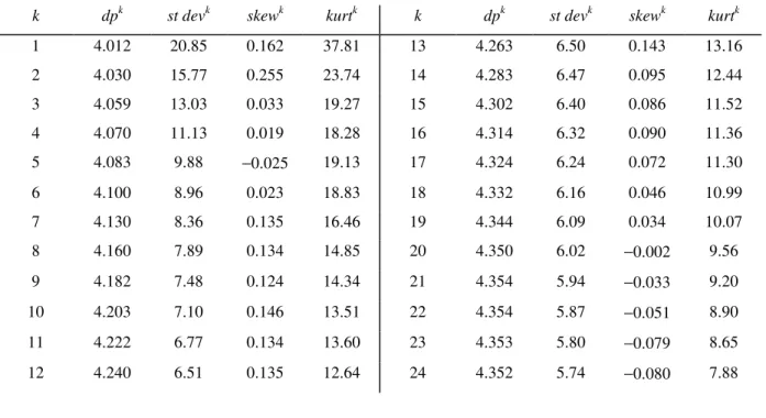
In Table 1 we report the average moments of the distribution of the k−month price changes of

85 components RPI over the period January 1987 - December 1998 (144 observations) for

values of k between 1 (monthly inflation) and 24 months (two yearly inflation).

Table 1 : Average moments of the distribution of the k−month price changes of 85

components RPI (annualised rates)

k dpk st devk skewk kurtk k dpk st devk skewk kurtk

1 4.012 20.85 0.162 37.81 13 4.263 6.50 0.143 13.16

2 4.030 15.77 0.255 23.74 14 4.283 6.47 0.095 12.44

3 4.059 13.03 0.033 19.27 15 4.302 6.40 0.086 11.52

4 4.070 11.13 0.019 18.28 16 4.314 6.32 0.090 11.36

5 4.083 9.88 −0.025 19.13 17 4.324 6.24 0.072 11.30

6 4.100 8.96 0.023 18.83 18 4.332 6.16 0.046 10.99

7 4.130 8.36 0.135 16.46 19 4.344 6.09 0.034 10.07

8 4.160 7.89 0.134 14.85 20 4.350 6.02 −0.002 9.56

9 4.182 7.48 0.124 14.34 21 4.354 5.94 −0.033 9.20

10 4.203 7.10 0.146 13.51 22 4.354 5.87 −0.051 8.90

11 4.222 6.77 0.134 13.60 23 4.353 5.80 −0.079 8.65

12 4.240 6.51 0.135 12.64 24 4.352 5.74 −0.080 7.88

The sample moments in Table 1 indicate that the distribution of price changes is non-normal,

skewed and highly leptokurtic. This result was also found by Bryan and Cecchetti (1996,

1999) and Roger (1997) in US, Japan, and New Zealand inflation data respectively, but with a

difference. In their case they found positive skewness whereas we find a varying (and lower)

skewness. An important factor here maybe that their datasets cover longer periods of time and

include the 1970s whereas our dataset does not. The kurtosis of these distributions is very

high and decreases considerably with k, varying from 37.81 for monthly inflation to 12.63 for

annual inflation and to 7.88 for two yearly inflation. Some of the variations in skewness and

kurtosis are attributable to taking non seasonal differences in price series with seasonal

We will use k=12, annual inflation rate, as in many other studies and official publications,

thus avoiding the issue of (fixed) seasonal adjustment and decreasing transitory noise (as

discussed in Cecchetti (1997))4. Considering k=12, the distribution of annual inflation

changes is negatively skewed in the periods April 1991 to March 1994, December 1995 to

June 1997, and from October 1998 (see Figure 1), with an absolute minimum of −6.399 in

December 1996. In these periods, the number of large price decreases was greater than the

number of large price increases. The absolute maximum was 4.376 in March 1995. Kurtosis

was particularly high over two periods (August 1994 to June 1995 and October 1996 to June

1997) and again from November 1998 (see Figure 2) with an absolute maximum of 79.79 in

January 1997. Some idea of the appropriate scale for these measures is given by their

properties in samples from a normal distribution, where skewk would have mean 0 and

variance 6, while kurtk would have mean 3 and variance 24.

Given these characteristics of the sample distribution, a more robust estimator of the central

tendency is the weighted sample median, or 50% percentile, (see Figure 3). The median of the

annual inflation rate is (tends to be) lower than the inflation rate when there is positive skew

and higher when there is negative skew in the sample distribution. This happens because when

the distribution is positively skewed, there are more large price increases than price decreases

and the size of the former is not taken into account in the calculations of the median. Whereas

other investigators often find positive skewness in the price changes distribution and therefore

a median that tends to be lower than the inflation rate, we find a mixed situation: the median

is above the rate of inflation over the periods April 1991 to March 1994, December 1995 to

June 1997, and from October 1998, when the sample distribution is negatively skewed, and

4

below it at all other times. One can consider the median as a particular case of a trimmed

mean.

3. Trimmed mean inflation

We consider a class of robust location measures known as α−trimmed means defined as

(indices t and k (=12) omitted)

( )

x w dp_{i i}

i I

=

−

∑

1

1 2α₁₀₀ α

( ) ( )

where the sample of price changes was first sorted into order and relabelled so that

dp_{( )1} <dp_{( )2} < <! dp_{( )m} together with their associated weights w(i). The set of observations to

be averaged, I_α, is the set of price changes dp(i) corresponding to the cumulative weight

W_j w dp_{i i}

i j

=

∑

( )

important particular cases are given by α =0%,x₀ ≡dp, the weighted sample mean, and

α =50%,x50, the weighted sample median. Note that the trimming is done in cross-section

for each month of the sample and therefore, potentially, the categories trimmed in a given

month will be different from those trimmed in any other month of the sample.

Following Bryan and Cecchetti (1996,1999) and Bryan et al. (1997), we use bootstrap

methods to determine the trimming point. The optimal trimming point α* is the trim that

minimises either of the two measures of efficiency used, MAD (mean absolute deviation) and

RMSE (root mean square error). As a benchmark to judge efficiency, we follow Cecchetti

(1997) and the references above and use the 36 month centred moving average inflation5 as

the point about which to measure MAD and RMSE. Bryan and Cecchetti (1999) and Mio and

Higo (1999), for example, have concluded that the procedure is quite robust to the choice of

number of months in the moving average which we also find. We then calculate the relative

price changes of each category with respect to the 36 month moving average of inflation (or

the deviations of each category inflation from the 36 month moving average of inflation),

meaning that we have a matrix of 132 observations on 85 categories for relative price changes

together with their weights, which are updated every year6. In Appendix II we describe in

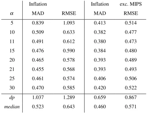
detail the bootstrap procedure used. In Figure 4 we plot the two measures of efficiency used,

MAD and RMSE, against α to determine the optimal trim and in Table 2, columns 2 and 3,

we report their values for selected values of α between 5% and 30% together with inflation

and median. The optimal trimming point is α* =21% chosen by both measures (minimises

both MAD and RMSE).

5

Implicit in this choice of benchmark is the assumption by Cecchetti (1997) that the 36 month centred moving average of inflation is a good approximation to the movements in the long-term trend in inflation, but as a low frequency trend it may not have the timeliness required by policy makers.

6

Table 2 : Optimal trimming point for inflation and inflation excluding MIPS

Inflation Inflation exc. MIPS

α MAD RMSE MAD RMSE

5 0.839 1.093 0.413 0.514

10 0.509 0.633 0.382 0.477

11 0.491 0.612 0.380 0.473

15 0.476 0.590 0.384 0.480

20 0.465 0.578 0.393 0.489

21 0.455 0.568 0.393 0.493

25 0.461 0.574 0.406 0.506

30 0.470 0.585 0.420 0.522

dp 1.037 1.289 0.659 0.867

median 0.523 0.643 0.460 0.571

NB: Rows for intermediate values of α calculated, but not shown.

Trimming improves considerably the efficiency of the inflation estimators. Even trimming 5%

off each tail reduces the MAD from 1.037 to 0.839 and the RMSE from 1.289 to 1.093, gains

of 19.1% and 15.2%, respectively. At the optimal 21%, the gains in efficiency are respectively

56.1% and 55.9%. (Using the median (α = 50%) as the central measure improves the

efficiency by 49.6% and 50.1%, respectively. Of course, 50% trimming about the median

gives MAD = RMSE = 0).

Some caution is needed in interpreting the location of the minima. Bootstrapping is random

re-sampling, and different experiments will produce different curves. One can estimate this

variability by a double bootstrapping, calculating the MAD and RMSE for 1000 replications,

then repeating the process 1000 times. The results are shown in Figure 5a and b, the bands

centre being the median and mean, which are coincidental for practical purposes. To take the

MAD, while the minimum is at α=22%, here the interval is 0.44080 to 0.47572, which

overlaps with the interval at α=14%. Thus we cannot clearly distinguish α=22% and α=14%.

One can attempt to reduce this variability by smoothing the MAD and RMSE curves. One way

of doing this is to render adjacent observations correlated by re-using the same random

numbers for different α values when re-sampling. The results are shown in Figures 6a and b.

There is similar uncertainty as to the precise location of the optimal trimming point.

In Figure 7 we plot α −trimmed inflation rates for α =10% and 15%, together with the

optimal trim 21% and inflation. The categories that were trimmed for each α are given in

Figure 8. The most trimmed categories were 'processed potatoes' (category No.24), MIPS

(No.41) and 'audio-visual equipment' (No.76), which were trimmed 91.7%, 95.5% and 99.2%

of the months respectively at the 21% optimal trim. The least trimmed components were

'restaurant meals' (No.31), 'take-aways and snacks' (No.33), 'DIY materials' (No.45), 'domestic

services' (No.59), 'other clothing' (No.64), and 'UK holidays' (No.84), which were all trimmed

less 5% of the months (minimum of 0.8% for Nos. 33 and 84) at the 21% optimal trim.

This optimal trimming point of 21% (meaning 21% trimmed off each tail to a total of 42%

excluded from the index) is quite high, perhaps reflecting the very high kurtosis of the annual

UK inflation series as discussed above. Using a different definition for UK inflation

(annualised monthly inflation excluding MIPS), sample period (1974-1997), and methodology

to calculate the optimal trimming point, Bakhshi and Yates (1999) estimate trimming points

of 17% using MAD and 47% using RMSE. Bryan et al. (1997) using monthly annualised

seasonally adjusted US inflation estimate an optimal trimming point of 7% and Bryan and

hand, Mio and Higo (1999) using annual Japanese inflation estimate 15%. One factor could be

the kurtosis of the distribution of category inflation. Bryan et al. (1997) show that ''the

efficient trim increases with the kurtosis of the data generating process''. Indeed, they report a

kurtosis of 12.64 for the monthly annualised US inflation whereas Bryan and Cecchetti (1999)

report a kurtosis of 31.25 for the monthly annualised Japanese inflation.

Unlike other studies, when we used the actual data to determine the optimal trim, i.e.,

calculate the minimum of MAD and RMSE of trimmed mean inflation for different values of

α with respect to the 36 month centred moving average of actual inflation (what Bryan and

Cecchetti (1999) call 'historical experiments'), we obtained a different and much smaller

optimal trim of 8% using the same benchmark (36 month moving average) and criteria (MAD

and RMSE).

We repeated the whole process for UK inflation excluding MIPS, i.e., inflation based on the

RPIX index. As shown in Table 2, columns 4 and 5, the optimal trimming point decreases to

11%. At the optimal 11%, the gains in efficiency are respectively 42.3% and 45.4%. Using the

median (α = 50%) improves the efficiency by 30.2% and 34.1%, respectively, where the

gains are smaller than when we use all the inflation components, as above. This trim should

be more comparable to the 15% trim used in some issues of the Bank of England's Inflation

Report (see footnote 1), but based on seasonally adjusted inflation data. The most trimmed

categories at the optimal 11% trim are still 'processed potatoes' (No.24), and 'audio-visual

equipment' (No.76), now trimmed only 85.6% and 91.7% of the months, respectively. Twelve

categories were never trimmed at the optimal 11% : 'sweets and chocolates' (No.23),

'restaurant meals' (No.31), 'take-aways and snacks' (No.33), 'DIY materials' (No.45), 'other

(No.64), 'chemist goods' (No.67), 'maintenance of motor vehicles' (No.70), 'other travel costs'

(No.75), and 'UK holidays' (No.84). Using the historical method, the optimal trim is reduced

to 4%. Exclusion of MIPS in the analysis excludes a volatile category which is usually

trimmed. This also induces (larger) fluctuations in the moving average, and thus decreases

MAD and RMSE. Given the flatness of much of these functions, it is not surprising that the

optimal trimming point moves considerably. It is not clear why it should be decreased.

In the above we follow Bryan and Cecchetti (1996,1999) and Bryan et al. (1997) and trim

symmetrically. However, we can allocate the total trim of 2α unequally to the two tails,

choosing the allocation which minimises the MAD and RMSE. Searching for an optimal

allocation from 0.5α, through 0.6α, ... up to 1.5α gives a minimum MAD of 0.458 at α=17%

(with a 22.1% / 11.9% split) and a minimum RMSE of 0.566 at α=16% (with a 20.8% /

11.2% split). The slight increase arises because we are re-using random deviates to smooth the

curves.

4. Conclusion

Using monthly data on the UK RPI we estimate a measure of core inflation based on a

trimmed mean with optimal trimming point α* =21% . This means that every month we trim

2×21% = 42% of the published index. The resulting measure diverges quite considerably from

the published inflation (see Figure 7) and, as discussed in text, is a more robust measure of

UK core inflation than the published inflation or other aggregates published by ONS. If we

base our calculations on the RPIX (RPI excluding MIPS) the optimal measure of core

inflation excludes a smaller proportion of the index : 2×11%=22%. However, problems

example when we compare our results with those obtained by Bakhshi and Yates (1999) for

the UK and with the results of investigators using data from other countries. It would appear

that we are some way from a clear and undisputed measure of core inflation.

It can be argued that trimming biases the index if a volatile and much excluded category

exhibits a significant trend: 'audio-visual equipment' (category No.76) is a candidate, with

consistent negative inflation throughout the period of analysis. Re-weighting schemes have

been used (see Lafleche (1997) and Wynne (1997,1999)), but these can also bias the index,

and suffer from aggregation problems. We have yet to find an appealing solution to this

problem.

5. References

Andrade, I.(1998), ''The History of the Cost of Living and RPI indices in the UK: 1914 to 1997'', mimeo, Department of Management, University of Southampton.

Bank of England, Inflation Report, 1993-..., various issues.

Bakhshi, H. and Yates, T. (1999), ''To trim or not to trim? An application of a trimmed mean inflation estimator to the United Kingdom'', Bank of England Discussion Paper.

Ball, L. and N.G. Mankiw (1995), ''Relative-price changes as aggregate supply shocks'',

Quarterly Journal of Economics, 110, pp.161-193.

Baxter, M.(ed.) (1998), The Retail Prices Index: Technical Manual, ONS, The Stationery Office, London.

BPP, British Parliamentary Papers, different years.

Bryan, M.F. and Cecchetti, S.G. (1996), ''Inflation and the distribution of price changes'', NBER Working Paper No.5793.

Bryan, M.F. and Cecchetti, S.G. (1999), ''The monthly measurement of core inflation in Japan'', Bank of Japan IMES Discussion Paper No.99-E-4.

Cecchetti, S.G. (1997), ''Measuring short-run inflation for central bankers'', Federal Reserve Bank of St. Louis Review, May/June, pp.143-155.

Haldane, A.G. (ed.) (1995), Targeting Inflation: A Conference of Central Banks on the Use of Inflation Targets, Bank of England, London.

Haldane, A.G. (1998), ''On inflation targeting in the United Kingdom'', Scottish Journal of Political Economy, 45, pp.1-32.

Lafleche, T. (1997), ''Statistical measures of the trend rate of inflation'', Bank of Canada Review, Autumn, pp. 29-47.

Mio, H. and Higo, M. (1999), ''Underlying inflation and the distribution of price changes : Evidence from the Japanese trimmed mean CPI'', Bank of Japan IMES Discussion Paper No.99-E-5.

Office for National Statistics (ONS), Business Monitor MM23 - Retail Price Index, 1993-..., various issues. (initially published by the CSO).

Roger, S. (1997), ''A robust measure of core inflation in New Zealand, 1949-96'', Reserve Bank of New Zealand Discussion Paper G97/7.

Roger, S. (1998), ''Core inflation: Concepts, uses and measurement'', Reserve Bank of New Zealand Discussion Paper G98/9.

Shiratsuka, S. (1997), ''Inflation measures for monetary policy: Measuring the underlying inflation trend and its implication for monetary policy implementation'', Monetary and Economic Studies, December 1997, pp.1-26.

Stuart, A. and Ord, J.K. (1994), Kendall's Advanced Theory of Statistics, Volume I, Distribution Theory, 6th edition, Edward Arnold.

Wynne, M.A. (1997), ''Commentary'' on Cecchetti (1997), Federal Reserve Bank of St. Louis Review, May/June, pp.161-167.

Wynne, M.A. (1999), ''Core inflation: a review of some conceptual issues'', European Central Bank Working Paper Series, Working Paper No.5; and Chapter 1 in Measures of underlying inflation and their role in the conduct of monetary policy - Proceedings of the workshop of central bank model builders, Bank for International Settlements, Basel, June.

6. Appendices

6.1. Appendix I

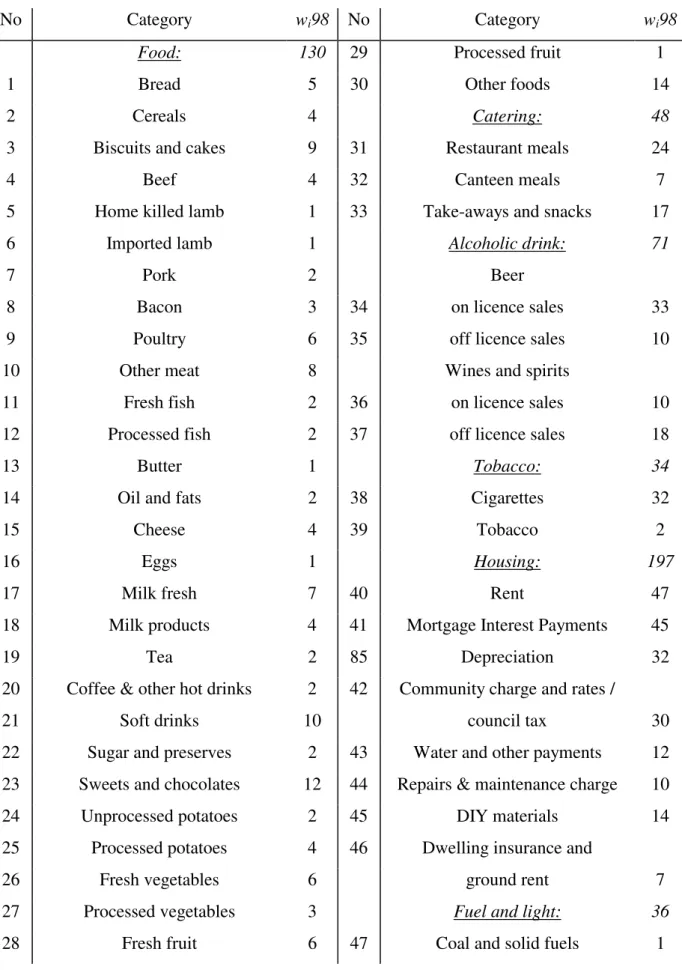
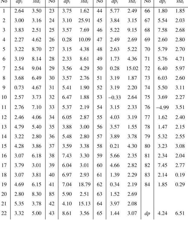
In Table A1 we list the 85 categories of the UK RPI, together with their 1998 weights. In

Table A2 we list the descriptive statistics of the annual inflation of each of the 85 categories

Table A1: RPI Categories description and 1998 weights

No Category wi98 No Category wi98

Food: 130 29 Processed fruit 1

1 Bread 5 30 Other foods 14

2 Cereals 4 Catering: 48

3 Biscuits and cakes 9 31 Restaurant meals 24

4 Beef 4 32 Canteen meals 7

5 Home killed lamb 1 33 Take-aways and snacks 17

6 Imported lamb 1 Alcoholic drink: 71

7 Pork 2 Beer

8 Bacon 3 34 on licence sales 33

9 Poultry 6 35 off licence sales 10

10 Other meat 8 Wines and spirits

11 Fresh fish 2 36 on licence sales 10

12 Processed fish 2 37 off licence sales 18

13 Butter 1 Tobacco: 34

14 Oil and fats 2 38 Cigarettes 32

15 Cheese 4 39 Tobacco 2

16 Eggs 1 Housing: 197

17 Milk fresh 7 40 Rent 47

18 Milk products 4 41 Mortgage Interest Payments 45

19 Tea 2 85 Depreciation 32

20 Coffee & other hot drinks 2 42 Community charge and rates /

21 Soft drinks 10 council tax 30

22 Sugar and preserves 2 43 Water and other payments 12

23 Sweets and chocolates 12 44 Repairs & maintenance charge 10

24 Unprocessed potatoes 2 45 DIY materials 14

25 Processed potatoes 4 46 Dwelling insurance and

26 Fresh vegetables 6 ground rent 7

27 Processed vegetables 3 Fuel and light: 36

No Category wi98 No Category wi98

48 Electricity 18 Fares and other travel costs: 20

49 Gas 16 73 Rail fares 4

50 Oil and other fuels 1 74 Bus and coach fares 5

Household goods: 72 75 Other travel costs 11

51 Furniture 20 Leisure goods: 46

52 Furnishings 13 76 Audio-visual equipment 10

53 Electrical appliances 9 77 Tapes and discs 6

54 Other household equipment 7 78 Toys, photographic and

55 Household consumables 15 sport goods 11

56 Pet care 8 79 Books and newspapers 12

Household services: 54 80 Gardening products 7

57 Postage 2 Leisure services: 61

58 Telephones, telemessages, etc. 16 81 TV licences and rentals 10

59 Domestic services 9 82 Entertainment and other

60 Fees and subscriptions 27 recreation 18

Clothing and footwear: 55 83 Foreign holidays 25

61 Men's outwear 11 84 UK holidays 8

62 Women's outwear 18

63 Children's outwear 6

64 Other clothing 10 Total 1000

65 Footwear 10

Personal goods and services 40

66 Personal articles 11

67 Chemists goods 19

68 Personal services 10

Motoring expenditure: 136

69 Purchase of motor vehicles 53

70 Maintenance of motor vehicles 24

71 Petrol and oil 39

Notes:

'wi98' are the 1998 weights for the 85 categories expressed out of 1000. The total

weight for each of the 14 main categories is given in italics next to its title.

The ONS has published price indices for all these categories since 1987 (January

1987=100) except for categories 83 ('Foreign holidays') which started in January 1993

(January 1993=100), 84 ('UK holidays') in January 1994 (January 1994=100) and 85

('Depreciation') in January 1995 (January 1995=100).

Adjustments were made to five categories in Food and two in Alcoholic drink:

− ONS subdivides 'Lamb', 'Fish', 'Potatoes', 'Vegetables' and 'Fruit' into two different

categories (typically 'fresh' and 'processed') with two different weights, but publishes price

indices only for the aggregate and for the 'fresh' category. In each case we calculated the price

index for each 'processed' category out of the aggregate category, and used only the 'fresh' and

'processed' categories in our dataset;

− In Alcoholic drink, the ONS publishes price indices for total 'Beer' and 'Wine and

spirits' sales, together with price indices for those sales disaggregated in 'on' and 'off' licence

Table 2A : Average mean and stand deviation of annual category inflation rate

No dpi stdi No dpi stdi No dpi stdi No dpi stdi

1 2.64 3.50 23 3.75 1.62 44 5.77 2.49 66 1.80 1.85

2 3.00 3.16 24 3.10 25.91 45 3.84 3.15 67 5.54 2.03

3 3.83 2.51 25 3.57 7.69 46 5.22 9.15 68 7.58 2.68

4 2.27 4.62 26 0.28 10.09 47 2.49 2.69 69 2.60 2.80

5 3.22 8.70 27 3.15 4.38 48 2.63 5.22 70 5.79 2.70

6 3.19 8.14 28 2.33 8.61 49 1.73 4.36 71 5.76 4.71

7 2.54 9.04 29 3.56 4.29 50 0.28 15.02 72 6.40 5.97

8 3.68 6.49 30 3.57 2.76 51 3.19 1.87 73 6.03 2.60

9 0.73 4.67 31 5.41 1.90 52 3.19 2.20 74 5.50 3.11

10 2.57 3.73 32 6.47 1.88 53 −0.33 2.64 75 3.69 2.27

11 2.76 7.10 33 5.37 2.19 54 3.15 2.33 76 −4.99 3.51

12 2.46 4.06 34 6.05 2.87 55 4.03 3.19 77 1.62 2.40

13 4.79 5.40 35 3.88 3.00 56 3.57 1.55 78 1.47 2.15

14 3.22 2.80 36 5.48 2.80 57 3.89 3.78 79 5.32 2.55

15 4.28 3.86 37 3.59 3.38 58 0.21 4.30 80 3.23 3.08

16 3.07 6.18 38 7.43 3.30 59 5.66 2.35 81 2.34 2.04

17 3.79 3.01 39 6.04 3.01 60 4.66 2.82 82 7.45 2.77

18 3.07 3.81 40 6.97 2.93 61 1.39 2.29 83 2.14 0.19

19 4.69 6.15 41 7.04 18.79 62 0.34 2.19 84 1.85 0.29

20 2.80 8.30 85 5.90 2.51 63 1.52 2.69

21 5.35 3.78 42 4.10 15.13 64 3.97 2.08

6.2. Appendix II

Bootstrap Methodology

Following Bryan and Cecchetti (1996,1999) and Bryan et al.(1997) we set up a matrix of

relative prices (log price deviations) with respect to the 36 month centred moving average

inflation for each category of inflation. The matrix has 132 rows (monthly observations) and

85 columns (categories) and general element xj of log price deviations from the 36 month

centred moving average for that column. In each experiment we draw randomly one

observation from each category, i.e., one draw from each column of the matrix, weighted by

the column (category) weight for that year, (the weights are re-normalised in each draw to sum

to 1000). We use n = 10,000 replications, thus generating 10,000 ''observations'', and calculate

trimmed inflation for a given α. Then we compute two measures of efficiency about zero: the

MAD (mean absolute deviation)

MAD x

n

j t n

α

α

=

∑

and the RMSE (root mean square error)

( )

RMSE x

n

j t n

α

α

=

∑

2 1

The process is repeated for each value of α from 5% to 30%, enabling us to plot MAD_α and

Fig.1

Skewness : January 1988 - December 1998

-8 -6 -4 -2 0 2 4 6

Jan-88 Jan-89 Jan-90 Jan-91 Jan-92 Jan-93 Jan-94 Jan-95 Jan-96 Jan-97 Jan-98

Fig. 2

Kurtosis : January 1988 - December 1998

0 10 20 30 40 50 60 70 80 90

Fig.3

Inflation and Median : January 1988 - December 1998

0 2 4 6 8 10 12

Jan-88 Jan-95

dp

median

Fig. 4

Optimal trimming point : MAD and RMSE

0 0.2 0.4 0.6 0.8 1 1.2

5 6 7 8 9 10 11 12 13 14 15 16 17 18 19 20 21 22 23 24 25 26 27 28 29 30

alpha

MAD

Fig. 5a

MAD : 5% and 95% doublebootstrap confidence bands

0.000000 0.100000 0.200000 0.300000 0.400000 0.500000 0.600000 0.700000 0.800000 0.900000 1.000000

5 6 7 8 9 10 11 12 13 14 15 16 17 18 19 20 21 22 23 24 25 26 27 28 29 30

alpha

MAD

5%

95%

Fig. 5b

RMSE : 5% and 95% doublebootstrap confidence bands

0.000000 0.200000 0.400000 0.600000 0.800000 1.000000 1.200000

5 6 7 8 9 10 11 12 13 14 15 16 17 18 19 20 21 22 23 24 25 26 27 28 29 30

alpha

RMSE

5%

Fig. 6a

MAD : double bootstraping confidence bands (same random numbers)

0.000000 0.100000 0.200000 0.300000 0.400000 0.500000 0.600000 0.700000 0.800000 0.900000 1.000000

5 6 7 8 9 10 11 12 13 14 15 16 17 18 19 20 21 22 23 24 25 26 27 28 29 30

alpha

MAD 5% 95%

Fig. 6b

RMSE : double bootstrap confidence bands (same random numbers)

0.000000 0.200000 0.400000 0.600000 0.800000 1.000000 1.200000

5 6 7 8 9 10 11 12 13 14 15 16 17 18 19 20 21 22 23 24 25 26 27 28 29 30

alpha

RMSE

5%

Fig. 7

Trimmed Mean Inflation : January 1988 - December 1998

0 2 4 6 8 10 12

Jan-88 Jan-95

10% trim

15% trim

21% trim

dp

Fig. 8a

Trimmed Categories : Food, Catering, Alcoholic drink and Tobacco (in %)

0 20 40 60 80 100

1 4 7 10 13 16 19 22 25 28 31 34 37

Categories

%

10% trim

15% trim

Fig. 8b

Trimmed Categories : Housing to Leisure services (in %)

0 20 40 60 80 100 120

40 43 47 51 55 59 63 67 71 75 79 83

Categories

%

10% trim

15% trim