Technical analysis on foreign exchange markets: MACD and RSI

TECHNICAL ANALYSIS ON FOREIGN EXCHANGE MARKETS:

MACD AND RSI

João Pedro Valdez Lancinha Cardoso

Project submitted as partial requirement for the conferral of MSc in Finance

Supervisor:

Professor Pedro Manuel de Sousa Leite Inácio, Assistant Professor, ISCTE Business School, Finance Department

TECHNICAL ANALYSIS ON FOREIGN EXCHANGE MARKETS:

MACD AND RSI

João Pedro Valdez Lancinha Cardoso

Project submitted as partial requirement for the conferral of MSc in Finance

Supervisor:

Professor Pedro Manuel de Sousa Leite Inácio, Assistant Professor, ISCTE Business School, Finance Department

II

Index

1.1. Technical analysis – Overview ... 1

1.2. The origin of technical analysis - The Japanese and the rice market ... 2

1.3. Dow Theory ... 3

1.4. Technical analysis as a method to predict future prices ... 6

1.5. Forex – Brief history and current statistics ... 8

2. Hypotheses ... 11

3. Data ... 11

4. Methodology ... 12

4.1. Moving Average Convergence/Divergence (MACD) ... 12

4.2. Relative Strength Index (RSI) ... 15

4.3. Data setting, testing and evaluation of results ... 17

5. Presentation and analysis of results ... 19

5.1. MACD test results ... 19

5.2. RSI test results ... 24

5.3. The shift in USD price ... 29

5.4. Discussion of results ... 30

6. Conclusion ... 31

7. References ... 33

III

Figure Index

Figure 1 - Candlestick of EUR/USD price (January 1st, 2018- June 30th, 2018) ... 3

Figure 2 - MACD for EUR/USD (January 1st, 2018 - December 31st, 2018) ... 13

Figure 3 - RSI for EUR/USD (January 1st, 2018 - December 31st, 2018) ... 15

Figure 4 - MACD vs B&H - EUR/USD (January 1st, 2009 – December 31st, 2018) ... 21

Figure 5 - MACD vs B&H - JPY/USD (January 1st, 2009 – December 31st, 2018) ... 22

Figure 6 - MACD vs B&H - GBP/USD (January 1st, 2009 – December 31st, 2018) ... 22

Figure 7 - MACD vs B&H - AUD/USD (January 1st, 2009 – December 31st, 2018) ... 23

Figure 8 - MACD vs B&H - CAD/USD (January 1st, 2009 – December 31st, 2018) ... 24

Figure 9 - RSI vs B&H - EUR/USD (January 1st, 2009 – December 31st, 2018) ... 26

Figure 10 - RSI vs B&H - JPY/USD (January 1st, 2009 – December 31st, 2018) ... 26

Figure 11 - RSI vs B&H - GBP/USD (January 1st, 2009 – December 31st, 2018) ... 27

Figure 12 - RSI vs B&H - AUD/USD (January 1st, 2009 – December 31st, 2018) ... 28

Figure 13 - RSI vs B&H - CAD/USD (January 1st_{, 2009 – December 31}st_{, 2018) ... 28}

Table Index

Table 2 - Explanation of the contents of MACD and RSI summary tables ... 18

Table 3 - MACD overall results (January 1st, 2009 - December 31st, 2018) ... 20

Table 4 - RSI overall results (January 1st, 2009 - December 31st, 2018) ... 25

Table 5 - Profitability of MACD, RSI and B&H (June 30th, 2014) ... 29

Formula Index

Equation 2 - Exponential Moving Average (EMA) ... 14

Equation 3 - Smoothing Constant (alpha) ... 14

Equation 4 - Simple Moving Average for MACD computation (SMA) ... 14

Equation 5 - Signal Line ... 14

Equation 6 - RSI ... 16

Equation 7 – RS ... 16

IV

Appendix Index

Appendix I – Global Forex turnover - Daily Average by currency pair (April 2019) .... 35

Appendix II – EUR/USD price (January 1st, 2009 - December 31st, 2018) ... 36

Appendix III – JPY/USD price (January 1st, 2009 - December 31st, 2018) ... 36

Appendix IV - GBP/USD price (January 1st, 2009 - December 31st, 2018) ... 37

Appendix V - AUD/USD price (January 1st, 2009 - December 31st, 2018) ... 37

Appendix VI - CAD/USD price (January 1st, 2009 - December 31st, 2018) ... 38

Appendix VII - EUR/USD MACD (January 1st, 2009 - December 31st, 2018) ... 38

Appendix VIII - JPY/USD MACD (January 1st, 2009 - December 31st, 2018) ... 39

Appendix IX - GBP/USD MACD (January 1st, 2009 - December 31st, 2018) ... 39

Appendix X - AUD/USD MACD (January 1st, 2009 - December 31st, 2018) ... 40

Appendix XI – CAD/USD MACD (January 1st, 2009 - December 31st, 2018) ... 40

Appendix XII - EUR/USD RSI (January 1st, 2009 - December 31st, 2018) ... 41

Appendix XIII - JPY/USD RSI (January 1st_{, 2009 - December 31}st_{, 2018) ... 41}

Appendix XIV - GBP/USD RSI (January 1st, 2009 - December 31st, 2018) ... 42

Appendix XV - AUD/USD RSI (January 1st_{, 2009 - December 31}st_{, 2018) ... 42}

Appendix XVI - CAD/USD RSI (January 1st_{, 2009 - December 31}st_{, 2018) ... 43}

Acronyms and Abbreviations

AUD – Australian Dollar B&H – Buy and Hold CAD – Canadian Dollar CP – Closing Price

DMI - Directional Movement Indicator EMA – Exponential Moving Average EUR - Euro

FOREX or FX– Foreign Exchange Market GBP - British Pound

JPY – Japanese Yen

MACD - Moving Average Convergence Divergence OTC – Over-the-counter

RSI – Relative Strength Index SMA – Simple Moving Average USD – United States Dollar

V

Abstract

For many years, technical analysis has been a topic of discussion regarding its contribution to rational investment decisions in financial markets. In an era where computational power is greater than ever and so many market analysis tools have been developed, one may question if the least sophisticated indicators, widely used in the past, remain relevant to current traders or if, on the other hand, their ability to predict investment opportunities lost their value. In this empirical study, we assess the individual performance of Moving Average Convergence/Divergence (MACD) and Relative Strength Index (RSI) in the Forex Market, specifically on the top five currency pairs currently traded, namely, USD/EUR, USD/JPY, USD/GBP, USD/AUD and USD/CAD, using daily closing prices from January 1st, 2009 to December 31st, 2018. Based on the signals collected from the tested indicators, we simulate long and short orders using a predetermined capital amount in order to assess the overall performance and accumulated profitability of each indicator. We conclude that, for both indicators, the results are ambiguous as they differ depending on the currency pair or the period for which they are applied to. Therefore, it is not possible to confirm that these tools can systematically outperform the market indicating profitable decisions in the covered context.

JEL classification: F31, G11

Key words: Foreign Exchange Markets, Technical Analysis, Moving Average Convergence/Divergence (MACD), Relative Strength Index (RSI)

VI

Resumo

Há muito tempo que a análise técnica tem sido um tópico de discussão relativamente à sua contribuição para decisões racionais de investimento nos mercados financeiros. Numa era em que o poder computacional é maior do que nunca e tantas ferramentas de análise de mercado foram desenvolvidas, pode-se questionar se os indicadores menos sofisticados, amplamente utilizados no passado, permanecem relevantes para os investidores atuais ou se, por outro lado, a sua capacidade de prever oportunidades de investimento perderam o seu valor. Neste estudo empírico, avaliamos o desempenho individual dos indicadores Convergência/Divergência das Médias Móveis (MACD) e Índice de Força Relativa (RSI) no mercado cambial, especificamente nos cinco principais pares de divisas atualmente negociados, nomeadamente, USD/EUR, USD/JPY, USD/GBP, USD/AUD e USD/CAD, usando preços de fecho diários de 1 de janeiro de 2009 a 31 de dezembro de 2018. De acordo com os sinais obtidos dos indicadores testados, simulamos ordens de compra e venda usando um capital predeterminado de forma a avaliar o desempenho global e a rentabilidade acumulada de cada indicador. Concluímos que, para ambos os indicadores, os resultados são ambíguos, uma vez que diferem consoante o par de divisas ou o período para o qual são aplicados. Desta forma, não é possível confirmar que aqueles indicadores superam o mercado sistematicamente indicando decisões rentáveis no contexto abordado.

Classificação JEL: F31, G11

Palavras-chave: Mercado Cambial, Análise Técnica, Convergência/Divergência das Médias Móveis (MACD), Índice de Força Relativa (RSI)

VII

Introduction

The ability of technical analysis to generate rational, well-informed and profitable investment decisions in financial markets is a topic far from having a consensus view.

Many argue that technical analysis does not add value to investment decisions since they defend that markets are fully efficient and, therefore, there is no misalignment between price adjustments and the available information. Therefore, the opportunity to identify investment opportunities through the study of historical prices or trends is null. On the other hand, others argue that technical analysis is a useful tool for any investor and should be used exclusively or in combination with fundamental analysis in order to take advantage of as much information as possible and, thereby, outperform the market, in an attempt to anticipate asset price adjustments. The foreign exchange market is the most liquid financial market and where the largest daily volume of transactions occurs and, therefore, where the investment decision process is particularly challenging due to its dynamic profile.

The objective of this empirical study is to evaluate if MACD (Moving Average Convergence/Divergence) and RSI (Relative Strength Index), two of the most applied and well-known tools of technical analysis, are still relevant in the current context of foreign exchange markets (Forex), given all the computational power available to investors nowadays, particularly when investing in the currency pairs with the highest transaction volumes in the market, namely, the U.S. Dollar versus Euro, Japanese Yen, British Pound, Australian Dollar and Canadian Dollar.

We start this study by presenting an overview on the subjects of technical analysis and Forex. In that sense, we cover the definition of technical analysis and forex, their purpose and a brief history from their creation until their role in financial markets nowadays, including the most important players and events in their development and the main studies performed on the matters.

After the introduction of the topics covered, we present the hypotheses tested in this empirical study and the details of the data collected for that purpose.

Through the simulation of trading decisions aided by the two analysed indicators, we determine if the signs of these tools actually spot triggers for the beginning of long and short positions

VIII with positive trading results when comparing to a Buy and Hold strategy (B&H). To do so, we use a fictitious starting capital amount that is invested exclusively according to the tools' indications over a defined period. After that period, all gains and losses are summed resulting in a net gain or loss in relation to the amount of the final capital if the B&H strategy is followed. The main results are then discussed in a detailed presentation of the impact of each indicator on each of the currency pairs studied.

In the end, we conclude that the results are ambiguous as they diverge depending on the currency pair or the period studied. Thus, we cannot confirm that these tools can systematically outperform the market indicating profitable decisions in the covered context.

1

1. Literature Review

1.1. Technical analysis – Overview

In the publication of Murphy (1999), the author defines that “Technical analysis is the study of

market action, primarily through the use of charts, for the purpose of forecasting future price trends.”.

Within the definition given by Murphy (1999), there are three underlying principles that the author claims to be the premises of technical analysis. The premises are that “Market action

discounts everything”; “Prices move in trends” and “History repeats itself”.

Technicians make their analysis assuming that any phenomenon that may influence prices is reflected in the price itself and, therefore, the study of price action is the only variable that matters in forecasting price trends. This is, aspects like political, social, psychological or other factors, that indeed have influence in the price movements, are already mirrored in the market as prices fluctuate through the dynamism of supply and demand. This explains the first premise of technical analysis.

The overall purpose, in a simplistic approach, of most technical analysis tools and techniques is to determine if the market is starting a trend (bullish, bearish or sideways) in order to trade inside that trend and trying to determine when the trend will reverse. Thus, the idea that markets move in trends is critical when considering technical analysis.

It is a general accepted idea that many phenomena in the world are cyclical and tend to occur from time to time. For instance, it is commonly known that economical conjunctures or even fashion tendencies tend to occur in a range of time, repeating themselves over the years. These events are explained within the studies of human psychology. Therefore, a way to understand the present and future is by studying the past and observing what happened in a certain situation that may possibly happen again in the future. This approach is observed in certain patterns in price charts that reveal market trends occurring in the past and repeating themselves over time and, consequently, giving technicians comfort in the idea that it will happen again.

2

1.2. The origin of technical analysis - The Japanese and the rice market

coupons represented the first future contracts in the history of markets. The Dojima Rice

Exchange is acknowledged as the first futures market. This was the background that led to the

development of technical analysis.

In the lead of rice trade and price analysis was a man called Munehisa Homma that was born in a very wealthy family with big rice farms and power. People like Homma were called

damyio’s2. Thus, Homma had easy access to rice’s price information and, additionally, he kept years of weather information and spent a lot of time studying the psychology of investors becoming very successful in rice trading. From Homma’s studies and methodology the

candlestick analysis 3 emerged becoming the first form of technical analysis.

Although candlestick analysis was well known in Asia for decades, it only arrived to the West by the hand of Steve Nison, a Wall Street investor, in the late 80’s. Nison started to study this type of analysis after seeing a Japanese broker looking at a candlestick chart and analysing patterns created by those candlesticks (Nison, 2001).

1 _{“Since there was no currency standard… rice became the defacto medium of exchange. A daimyo}2 _needing

money would send is surplus rice to Osaka where it would be placed in a warehouse in his name. He would be given a coupon as a receipt for this rice. He could sell this rice coupon whenever he pleased.” (Nison, 2001).

2_{“The word "daimyo" comes from the Japanese roots dai, meaning "big or great," and myo, or "name," so "great}

name." In this case, however, "myo" means something like "title to land," so the word really refers to the daimyo's large landholdings. The equivalent in English would be "lord." (Szczepanski, n/a)”.

3_{Candlestick analysis is an analysis based on charts that illustrate the evolution of past prices through a sequence}

3

Figure 1 - Candlestick of EUR/USD price (January 1st_{, 2018- June 30}th_{, 2018)}

Source: (Reuters, 2019)

Nevertheless, candlestick analysis is just one form of technical analysis. Actually, with the expansion of computer systems allied with the possibility of getting instantaneous access to a massive amount of financial information, technical analysis become much more than reading charts in a paper sheet.

1.3. Dow Theory

Dow Theory derives from a series of articles, published by Charles Dow in the Wall Street Journal by the end of the XIX century and the beginning of the XX century. The theories

published during that time are still commonly accepted as the basis for technical analysis nowadays.

Charles Dow was a journalist and a financial analyst, born in 1851 in Connecticut, United States of America. In his early twenties, Dow worked in several newspapers and was notable for his carefully written and well-documented articles, which led him to be invited to a Colorado financiers group where he wrote several articles regarding silver mines investment opportunities, among other topics. In 1880, Charles Dow moved to New York City where he

4 fully embraced financial journalism beginning as a business reporter in the New York Mail and

Express and later taking a job at Kiernan News Agency as editor.

In Kiernan News Agency he was joined by his former colleague Edward D. Jones as a reporter and in 1882, together, they left the agency and created the Dow Jones & Company, Inc, competing directly with their former news agency.

In the next years Dow and Jones were dedicated in writing daily reports about financial news, analysis of stock markets and forecasts, named as The Customer’s Afternoon News Letter. As the business grew, the publications got more extensive and became the predecessor of The Wall

Street Journal.

In mid-1884, Dow Jones & Company began to regularly publish the average closing prices of several stocks, including railways and manufacturing companies, that Charles Dow believed to be market representative and could be an accurate indication of the economy’s health, at that time. In 1897, two separate averages were created by Dow, one with industrial companies and the other with railway companies. Over the years, additional stocks were included in the industrial index and, in 1928, that index was represented by 30 stocks, the number that currently stands and by what is called the Dow Jones Industrial Average (encyclopedia.com, 2019). During his time in The Wall Street Journal, Charles Dow, published several articles on market behaviour that, one year after Dow’s death, in 1903, were compiled by Samuel Armstrong Nelson and published in a book entitled The ABC of Stock Speculation, (Nelson, 1903), there and then the term Dow Theory was first established.

As explained by Murphy (1999), the six basic tenets of The Dow Theory are: (i) the averages discount everything; (ii) the market has three trends; (iii) major trends have three phases (iv) the averages must confirm each other (v) volume must confirm the trend; and (vi) a trend is assumed to be in effect until it gives definite signals that it has reversed. The six tenets mentioned determine the ground assumptions in which technical analysis is based and from which it is possible to draw conclusions on future price trends by analysing observed past market prices.

One of the most important assumptions of Dow Theory, and the first enumerated, is that at a given point in time the market price reflects all the information known to investors at that time, whether that information regards to the past, present or even some future event not yet occurred

5 that will certainly or possibly affect the market price of a given asset. Additionally, the impact of an unexpected event is almost instantaneously reflected in the market price as supply and demand are automatically corrected by that new piece of information. The way that capital markets are able to correct asset prices with the input of new information is known as ‘market efficiency’ (this subject is discussed in the next section).

Charles Dow also states that there are three kinds of market trends4 observed in the market and that major trends present three phases. The primary trend is a pattern that occurs over a longer period of time and determines the predominant price movement even if downward or upward price corrections occur at a certain point in time. A secondary trend corresponds to the corrections in the primary trend that last for shorter periods of time and are not so significant that can change the primary trend, this is, not changing the price main behaviour. Finally, the

minor trend corresponds to slightly price variations within the secondary trend that occur for

the shortest time of the three trends and do not have a significant influence in the market price. Especially in primary trends, Dow states that there are three phases that build a solid trend, being those: the accumulation phase which is obtained by the first investment decisions of experienced and more knowledgeable market players; the public participation phase where most investors, due to market behaviour and creation of a new trend, start to enter their positions originating a fast price evolution; and the distribution phase when public participation is well stablished and the volume of speculation is getting higher. It is called the distribution phase because more experienced investors, that had invested in the beginning of the trend formation, start to distribute again their assets before everyone else starts selling.

Concerning the averages and volume of transactions, Dow believes that, regarding the industrial and railways averages created at that time, a strong upward or downward signal was only present on the market if both averages converged in the same direction, one confirming the other and vice-versa. Additionally, the volume of transactions, although being considered a secondary indicator, also serves as a confirmation of an upward or downward signal as the volume of buying or selling transactions increase in a bullish or bearish market, respectively.

4 _{A trend is considered to be a market behaviour where the closing price of an asset regularly overcomes the}

higher closing price of previous observations during a determined period of time, called an ‘uptrend’, or in the other hand, a succession of lower closing prices than past observations, called a ‘downtrend’.

6

1.4. Technical analysis as a method to predict future prices

Capital market efficiency as presented by Fama (1970), states that current market prices fully reflect all the available information at that time and there is no range of price misalignment with the fair value of an asset. Eugene Fama published his work on this matter on The Journal of

Finance compiled in three publications: (Fama, 1970); (Fama, 1976) and (Fama, 1991).

On this matter, Bessembinder & Chan (1995) and Ito (1999) support the idea that for some emerging markets, market efficiency may not be fully applied in market prices like in more mature and well established markets and, therefore, technical analysis techniques may be used in order to achieve profitable investment decisions. Marshall, Cahan, & Cahan (2010) research on the matter support that there is no evidence that investment decisions based on technical analysis technics result in higher returns than the ones achieved by random data variation, when considering data snooping bias5. Nevertheless several practitioners affirm that technical analysis presents a predictive value.

In fact, Park & Irwin (2004) present a survey with the objective of reviewing theoretical and empirical studies on this matter. The empirical studies analysed include different technical analysis techniques such as technical trading systems, trading rules, statistical models and chart patterns and most part of the studies were gathered from working papers and academic journals published between 1960 and the date of the survey.

The conclusions reached point to the fact that technical analysis is commonly used by market practitioners in futures markets and foreign exchange markets with profitable results until the early 1990’s but lacks the evidence of empirical studies supporting the profitability of investment decisions using technical analysis techniques after that.

More recent researches such as the one by Chong & Ng (2008) and Xavier, Massoud, & Chien (2010) studied MACD and RSI tools in different market contexts. Chong & Ng (2008) studied the net returns using these tools over a 60-year dataset of the London Stock Exchange FT30 Index concluding positively on the profitability of both tools. Xavier, Massoud, & Chien (2010) tested the Mexican stock exchange on daily closing price data through the Mexican IPC Index

5 _{Data snooping bias refers to the misuse of data when, in order to support a conclusion, a large amount of variable}

combinations is used, increasing the probability of, by chance, those combinations of variables explaining the original conclusion. For more details on this topic, please refer to (Sullivan, Timmermann, & White, 1999).

7 with a dataset of 21 years, from January 1st_{, 1988 to June 30}th_{, 2009, concluding for the} profitability of the RSI tool and non-profitability of MACD.

Other researches were performed on Forex with the application of MACD technique. Yazdi & Lashkari (2013), tested the MACD in Forex, in a 10 year period, starting from January 1st, 2001 for the currency pairs of USD/EUR, GBP/USD, USD/CHF and USD/JPY, using hourly data and applying take profit6 and stop loss7 for each order in 30 pips. The conclusions reached are ambiguous as the same technique generated good and bad results depending on the traded currency pair, being the EUR/USD the only pair that generated profit.

A similar study was performed by Vajda (2014) with almost the same time period and the same indicator of the study of Yazdi & Lashkari (2013). In this study, the data was retrieved from 2000 to 2011 to EUR/USD currency pair and divided in 3 segments: 2000-2003 (dot-com

crisis8); 2004-2007 (non-crisis) and 2008 to 2011 (global financial crisis) with and without stop-loss and take-profit positions. The results were also inconclusive as the results differed for the different studied time-frames and strategies.

The periods tested in both studies mentioned above (studies of MACD technique in Forex) were influenced by major economic events such as the market recovery from the dot-com speculation bubble burst and the global recession between 2007 and 2009.

6 _{Take profit is an order to close a position, applied by investors, when the profit of that position reaches a}

predetermined value.

7 _{Stop Loss is an order to close a position, applied by investors, when the loss of that position reaches a}

predetermined value.

8 _{The dot-com crisis was a significant event for capital markets occurred between the years 2000-2003, when the}

speculation bubble around the market price of technological companies (mostly internet based), accumulated from 1994 to that date, burst, resulting in massive losses in market capitalization of several companies, some of which did not recovered and had to shut down.

8

1.5. Forex – Brief history and current statistics

A clear and broad definition of Forex is given by Lien (2009) as the author states that “The foreign exchange market is the generic term for the worldwide institutions that exist to exchange or trade currencies. Foreign exchange is often referred to as “forex” or “FX.”. The foreign exchange market is an over-the-counter (OTC) market, which means that there is no central exchange and clearinghouse where orders are matched. FX dealers and market makers around the world are linked to each other around the clock via telephone, computer, and fax, creating one cohesive market. (…) ”.

In the mid-eighteenth century was created a mechanism of establishing the relationship of prices based on a common commodity for all countries, gold, called the gold-standard (Copeland & Weston, 1988). This mechanism consisted in a system of a “fixed” exchange rate between currencies due to the fact that currencies were directly convertible to gold and vice-versa. Thus, it was assumed that the price of a monetary unit of a country applying the gold-standard could just drop until the gold export price itself. At that point, as it was assumed that the price could not be lower, speculators started to acquire the currency, based on the expectation that the price would go higher, strengthening the currency itself.

The fixed-rate mechanism of gold-standard was in place since its conception until the market’s instability growth during the First and Second World War.

In 1944, with the objective of stabilizing the markets and prevent further problems caused by the events that took place in the first half of the twentieth century, a conference was held, in Bretton Woods, New Hampshire, United States of America, in which 44 countries gathered to sign a new institutional arrangement with the purpose of governing international economy. From this event, among other outcomes, came the formation of two new institutions with the main purpose of regulating international economies that are still part of the economic scenery nowadays, the International Monetary Fund (IMF) and the World Bank. Other outcomes of the Bretton Woods agreement were the fixation of exchange rates between currencies and re-establishing the convertibility between monetary units and gold (Lien, 2009).

9 In short, Bordo (1992) explains that the Bretton Woods System9 _{implementation had the} objective of combining the advantages of gold-standard’s, based on a fixed rate system, and the advantages of floating rates creating a system of fixed-rates that could only be adjusted in the event of a fundamental disequilibrium of the markets.

That system was in place for several years until, due to several factors like the increase the shortage of gold reserves and the desire of governments to control the currency adjustment process (leading to the enforcement of import barriers and restrictions on lending and investing in foreign markets) and the speculative action of markets, led to the collapse of the Bretton Woods system. As a result, in 1971, the United States suspended the convertibility factor of their currency against gold and the U.S. Dollar price began to float according to its value against other currencies, ending the era of the Bretton Woods agreement. During the 70’s several countries also adopted the floating-rate system and, in 1978, as a result of a second amendment of the charter of the International Monetary Fund (IMF), a legalized system of floating exchange rates was created (Copeland & Weston, 1988).

The floating exchange rates, that are still the system in place in the current Foreign Exchange Markets, are not pegged to gold prices or to other currencies and their price fluctuation is the reflection of the forces of supply and demand for each currency.

According to the last published Triennial Central Bank Survey - Global foreign exchange

market turnover in 2019, published in September 2019 by the Bank of International Settlements

(2019), the global daily average volume of transactions, in foreign exchange trading, amounts to USD 6.6 trillion, in April 2019, up from USD 5.1 trillion, in April 2016. The U.S. Dollar is the major currency traded being on one side of 88% of all transactions.

9 _{A detailed study on the comparison between the Bretton Wood system and its preceding and subsequent systems}

10

OTC foreign exchange turnover

Net-net basis10_{, daily averages in April, in billions of}

US dollars

Instrument 2004 2007 2010 2013 2016 2019

Foreign exchange instruments

1,934 3,324 3,973 5,357 5,066 6,590 Spot transactions 631 1,005 1,489 2,047 1,652 1,987 Outright forwards 209 362 475 679 700 999

Foreign exchange swaps

954 1,714 1,759 2,240 2,378 3,202 Currency swaps 21 31 43 54 82 108

Options and other products11

119 212 207 337 254 294 Memo:

Turnover at April 2019 exchange

rates12 1,854 3,071 3,602 4,827 4,958 6,590 Exchange-traded derivatives 25 77 144 145 115 127 Table 1 - Global Forex turnover - Daily Average (April 2019)

Source: (Bank for International Settlements, 2019)

Regarding traded currency pairs, the five most transacted are U.S. Dollar versus Euro (24%), Japanese Yen (13.2%), British Pound (9.6%), Australian Dollar (5.4%) and Canadian Dollar (4.4%). Together those currency pairs represent 56.6% of forex trades, on a daily basis13. Based on the conclusions of previous studies on the performance of technical analysis, presented in section 3.4 Technical analysis as a method to predict future prices, and the data presented on this chapter, the objective of our empirical study is to assess the profitability of investment decisions based on technical analysis techniques in the Forex market where these techniques are widely applied, as it is also the market that presents a higher volume of transactions, particularly for the most liquid currency pairs traded.

10 _{Adjusted for local and cross-border inter-dealer double-counting (i.e. “net-net” basis).}

11 _{The category “other FX products” covers highly leveraged transactions and / or trades whose notional amount}

is variable and where a decomposition into individual plain vanilla components was impractical or impossible.

12 _{Non-US dollar legs of foreign currency transactions were converted into original currency amounts at average}

exchange rates for April of each survey year and then reconverted into US dollar amounts at average April 2019 exchange rates.

11

2. Hypotheses

The hypotheses considered for this empirical study are based on the ability of each studied indicator returning higher profitability levels than the Buy and Hold strategy, thus:

H0 – The return of the investment positions based on the application of the MACD tool is higher than the return of the application of the B&H strategy;

H0 – The return of the investment positions based on the application of the RSI tool is higher than the return of the application of the B&H strategy;

H1 – The return of the investment positions based on the application of the MACD tool is lower than the return of the application of the B&H strategy;

H1 – The return of the investment positions based on the application of the RSI tool is lower than the return of the application of the B&H strategy.

3. Data

Data was collected from Reuters database (2019) for the most common currency pairs traded in foreign exchange markets:

 EUR/USD (Euro / U.S. Dollar);

 JPY/USD (Japanese Yen / U.S. Dollar);  GBP/USD (British Pound / U.S. Dollar);  AUD/USD (Australian Dollar / U.S. Dollar);  CAD/USD (Canadian Dollar / U.S. Dollar).

For each currency pair, we collect daily closing exchange mid-rates from January, 1st _to December 31st_{, from 2009 to the end of 2018. Instead of collecting pip by pip}14 _{records, each}

14 _{The smallest unit of measure of the movement of an exchange rate. Almost every major currency change by the}

fourth decimal place of the price (0,0001). An exception is the Japanese Yen that changes its price only at two decimal places.

12 record represents the daily closing exchange rates in order to simplify the dataset collection and to reduce the amount of records collected.

We believe that this dataset represents the correct behaviour of the foreign exchange markets around the world and is not skewed by isolated events that could impact the normal dynamics of those markets and, therefore, impacting the conclusions reached in our empirical study. The total data set is comprised by roughly eighteen thousand records which includes the daily closing exchange mid-rate for the five currency pairs identified, from January 1st, 2009 to December 31st, 2018.

4. Methodology

4.1. Moving Average Convergence/Divergence (MACD)

4.1.1. MACD background

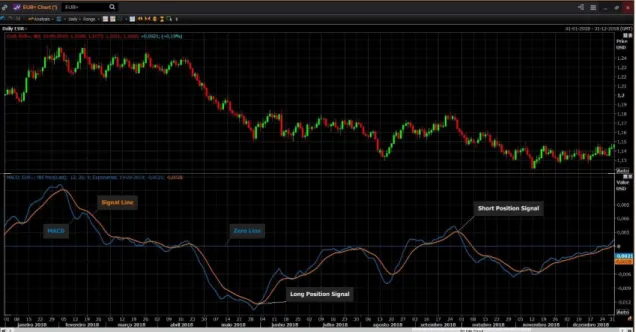
As mentioned by Murphy (1999) this tool was developed by Gerald Appel in the 60’s. The Moving Average Convergence/Divergence (MACD) tool is an indicator which combines two moving averages in order to sign buying and selling momentums. The first moving average is the result of the difference between a fast (shorter period of time) and a slow (longer period of time) exponential moving average (EMA) of the real market prices observed. The second one is an exponential moving average of the MACD itself, named the signal line, which is overlapped with the MACD. The signal to enter in a long position is triggered when the MACD crosses the signal line from a previous below position and triggers a short position when it crosses the signal line from a previous above position.

Additionally, as MACD represents the difference between a faster and a slower exponential moving average, the results will fluctuate around zero, both above and below that value. The above zero area represents the overbought area and the below zero area represents the oversold area. Thus, a strong long position signal is one that occurs in the oversold area. In contrast, a strong short position signal is one that occurs in the overbought area.

13

Figure 2 - MACD for EUR/USD (January 1st_{, 2018 - December 31}st_{, 2018)}

Source: (Reuters, 2019)

4.1.2. MACD computation

For the purpose of this study, the parameters set for the computation of MACD (measured by observations, meaning, the number of daily closing prices) were the following:

 Slower EMA: 26 observations;  Faster EMA: 12 observations;  Signal Line: 9 observations.

The parameters set represent the most common values used by traders when applying the MACD indicator.

As stated above, the MACD line corresponds to the difference between a slower and a faster EMA, thus:

𝑀𝐴𝐶𝐷 = 𝐸𝑀𝐴_𝑓− 𝐸𝑀𝐴_𝑠 (1)

Equation 1 - Moving Average Convergence/Divergence (MACD)

Being 𝐸𝑀𝐴_𝑓 the faster exponential moving average and 𝐸𝑀𝐴_𝑠 the slower exponential moving average.

The EMA for each period, is calculated by applying a smoothing constant (α) to the difference between the closing price of that period (CPn) and the EMA of the previous period (EMAn-1)

14 and adding EMAn-1. The smoothing constant (α) is a factor applied to the equation that enables the moving average to be more sensitive to recent observations, thus:

𝐸𝑀𝐴𝑛 = (𝐶𝑃𝑛− 𝐸𝑀𝐴𝑛−1) × ∝ +𝐸𝑀𝐴𝑛−1 (2) Equation 2 - Exponential Moving Average (EMA)

∝= 2

𝑡 + 1 (3)

Equation 3 - Smoothing Constant (alpha)

Where (t) corresponds to the number of observations we used to compute the EMA, in this case, 26 observations for EMAs and 12 observations for EMAf.

Notice that, the EMA for the first observation of the time period is just the Simple Moving Average (SMA) from which the following EMA’s are then calculated. This is, the first EMAs calculated is the SMA of the first 26 observations and the first EMAf is be the SMA of the first 12 observations.

The SMAt is the arithmetic mean of the (t) most recent observations. Again, 26 observations for the computation of EMAs and 12 observations for the EMAf:

𝑆𝑀𝐴_𝑡 =𝐶𝑃𝑛−𝑡+1+ ⋯ + 𝐶𝑃𝑛

𝑡 =

∑𝑛 𝐶𝑃_𝑛

𝑡=𝑛−𝑡+1

𝑡 (4)

Equation 4 - Simple Moving Average for MACD computation (SMA)

Finally, the Signal line is computed by calculating an Exponential Moving Average of the MACD itself. For the purpose of this study we used 9 observations, as stated previously:

𝑆𝑖𝑔𝑛𝑎𝑙 𝐿𝑖𝑛𝑒 = 𝐸𝑀𝐴𝑀𝐴𝐶𝐷,𝑡 (5)

15

4.2. Relative Strength Index (RSI)

4.2.1. RSI background

The RSI tool was developed by J. Welles Wilder, JR. and presented in his publication New

Concepts in Technical Systems, in 1978. According to Wilder (1978), “The Relative Strength

Index, RSI, is a tool which can add a new dimension to chart interpretation when plotted in conjunction with a daily bar chart.”.

The Relative Strength Index (RSI) is a momentum based tool that measures price fluctuations in order to predict if an asset is being overbought or oversold resulting, thus, in a speculation force for the price to decrease or increase, respectively. Thus, the trigger to enter in a long position appears when the tool indicates an oversold result and the trigger to enter in a short position appears when the tool indicates an overbought result.

The tool uses an average of profits and losses during a determined time range in order to plot the results in a scale from 0 to 100. An oversold signal occurs when RSI line passes below 30 in the scale and an overbought signal occurs when the RSI passes above 70 in that scale.

Figure 3 - RSI for EUR/USD (January 1st_{, 2018 - December 31}st_{, 2018)}

16

4.2.2. RSI computation

For the purpose of this study the parameters set for the computation of RSI were the following:  Oversold parameter: 30;

 Overbought parameter: 70;

 Number of observations: 14 days (closing prices).

The parameters set represent the most common values used by traders when applying the RSI tool.

The RSI line is obtained as follows:

𝑅𝑆𝐼 = 100 − 100 1 + 𝑅𝑆 (6) Equation 6 - RSI RS is obtained by: 𝑅𝑆 = 𝑆𝑀𝐴𝑡,𝑢𝑝 𝑆𝑀𝐴_{𝑡,𝑑𝑜𝑤𝑛} (7) Equation 7 – RS

Where SMAt,up or SMAt,down correspond to the Simple Moving Average of the daily gains or losses, respectively, occurred during the time period (t) set in the RSI parameters, in this case, 14 days closing prices.

The SMA is the arithmetic mean of the up closes gains or down closes losses during the (t) most recent observations. 𝑆𝑀𝐴_{𝑡,𝑢𝑝/𝑑𝑜𝑤𝑛}= 𝐺𝑎𝑖𝑛/𝐿𝑜𝑠𝑠𝑛−𝑡+1+ ⋯ + 𝐺𝑎𝑖𝑛/𝐿𝑜𝑠𝑠𝑛 𝑡 = ∑ 𝐺𝑎𝑖𝑛/𝐿𝑜𝑠𝑠𝑛 𝑛 𝑡=𝑛−𝑡+1 𝑡 (8)

Equation 8 - Simple Moving Average for RSI computation (SMA)

Where Gain/Loss is the positive/negative variation from Closing Price (CPn) and the Closing price from the previous period (CPn-1).

17

4.3. Data setting, testing and evaluation of results

In order to perform this empirical study we divide the collected dataset in two segments. We use Segment 1 for training the studied tools and Segment 2 for testing these tools.

We use the first segment, comprised by the first observations of the dataset (26 observations for MACD analysis and 14 for RSI analysis), to compute the behaviour of the tools through real market data. For the second segment, comprised by the majority of the dataset, we use the investment triggers retrieved from the tools in order to simulate investment decisions, this is, enter in long or short positions according with the tools results.

To accomplish the proposed test, a fictional amount of initial capital in a selected currency is settled as the basis amount to start investing, for the purpose of the study an amount of 100,000 USD. Then, we execute long or short positions according with the triggers of each tool and record the gains or losses of each position taken during the tested period, corresponding to the Segment 2, after exchanging all capital invested to the original currency, U.S. Dollars.

We acknowledge that the quality level of each tool is measured by the net amount of gains and losses resulting from the investment positions taken. Therefore, the results of each tool, applied to each currency pair, will be compared to accumulated gains and losses if the investor had followed a strategy of acquiring a currency, other than the one of its initial capital, in the first day of the tested time range and sold it back on the last day (Buy and Hold strategy).

In the case of accumulated net gains at the end of the period, when compared to the B&H strategy, the tools become interesting from the investor point of you. Otherwise, if those trading positions return an accumulated net loss, when compared to the B&H strategy, the tools fail their objective of helping in trading decisions.

18 Conclusions are summarized in tables with the following presentation:

Description Content

Total signals from tool Total number of observations where the tool marked entrance points for long and short positions.

Long signals Number of observations where the tool marked entrance points for long positions.

Short signals Number of observations where the tool marked entrance points for short positions.

Total orders Total number of orders to enter in long and short positions.

Long positions Number of orders to enter in long positions. Short positions Number of orders to enter in short positions.

Total closed positions Total number of closed positions with profitable or non-profitable result.

Closed gaining positions Number of positions closed with a profitable result. Closed losing positions Number of positions closed with a non-profitable result.

Initial Capital (MACD) Initial capital available to start trading with the MACD tool.

Trade gains Accumulated profit from positions closed with a profitable result. Trade losses Accumulated losses from positions closed with a non-profitable result.

Final Capital (MACD) Final capital available after the trading session with the MACD tool.

Total gains/losses ($) Net result of the trading session applying the MACD tool, in USD.

Total gains/losses (%) Net result of the trading session applying the MACD tool, as % of the initial capital.

Initial Capital Buy & Hold Initial capital available to start trading following the Buy & Hold strategy. Final Capital Buy & Hold Final capital available after the trading session following the Buy and Hold

strategy.

Total gains/losses B&H ($) Net result of the trading session following the Buy and Hold strategy, in USD. Total gains/losses B&H (%) Net result of the trading session following the Buy and Hold strategy, as % of

the initial capital.

Profitability MACD vs B&H ($)

Difference between the net result of the trading session with the MACD tool and the Buy and Hold strategy, in USD

Profitability MACD vs B&H (%)

Difference between the net result of the trading session with the MACD tool and the Buy and Hold strategy, in % of the initial capital

Table 2 - Explanation of the contents of MACD and RSI summary tables Source: Author

19 Additionally, the following assumptions are applied in our study:

i. The investor can trade one currency pair individually in each test (no cross investment between currencies);

ii. The investor cannot start a new long or short position unless the previous position is closed (no fragmentation of investment);

iii. The investor can trade during 24 hours per day, during week days (Forex markets are closed during weekends);

iv. The investor does not use Stop-Loss and Take-Profit orders (the order is active until the opposite signal is retrieved from the indicator);

v. No transaction costs are applied (the objective is to assess the pure performance of each tool without external factor influencing the results); and

vi. No spreads are applied between bid and ask prices (data collected reflect the average closing price for each day).

5. Presentation and analysis of results

The results of our empirical study are presented, initially, by summarizing the performance of each indicator followed by a disaggregated analysis by indicator and currency pair, in order to understand in detail the performance of each of those indicators by currency pair. After we present our overall discussions of results.

5.1. MACD test results

The application of MACD on the dataset resulted in a total amount of signals between 123 and 137, both long and short, depending on the currency pair tested. From the signals collected, between 25 and 29 investment positions were opened and closed resulting in gains or losses for the trader in each position as presented below (every closed position assumes that the tool marked a long/short position entrance point followed by the opposite signal).

Both total signals marked by the tool as well as positions closed, turn around 50% between long/short and profitable/non-profitable positions, in terms of number of events (with the

20 exception of GBP/USD for which 66% of total number of positions were profitable). Nevertheless, as it is possible to conclude by observing the information on Table 3, non-profitable positions exceed non-profitable ones in terms of net gains or losses. Thus, the application of MACD was not profitable by itself for any of the currency pairs studied.

Overall, the general negative returns observed on the MACD strategy are in line with the market behaviour during the tested period. This is, examining the results of B&H strategy, one can see that similar negative returns where generated for almost all the currency pairs (with the exception for AUD/USD where B&H strategy was profitable, with returns of 0.4% over the initial capital amount).Even though overall returns of MACD strategy were negative, the tool was able to beat the returns of the B&H strategy for EUR/USD (+6%), JPY/USD (+4%) and GBP/USD (+1%). For the remaining currencies, B&H had better results: AUD/USD (-8%) and CAD/USD (-4%).

Description* EUR/USD JPY/USD GBP/USD AUD/USD CAD/USD Total signals from tool 134 134 128 123 137

Long signals 63 (47%) 60 (45%) 64 (50%) 61 (50%) 69 (50%) Short signals 71 (53%) 74 (55%) 64 (50%) 62 (50%) 68 (50%)

Total closed positions 27 29 29 25 29

Closed gaining positions 14 (52%) 17 (59%) 19 (66%) 13 (52%) 14 (48%) Closed losing positions 13 (48%) 12 (41%) 10 (34%) 12 (48%) 15 (52%)

Initial Capital (MACD) 100,000 100,000 100,000 100,000 100,000

Trade gains 33,744 32,986 31,959 38,454 23,581

Trade losses (46,019) (46,606) (43,661) (46,196) (38,361) Final Capital (MACD) 87,724 86,381 88,297 92,258 85,220

Total gains/losses ($) (12,276) (13,619) (11,703) (7,742) (14,780)

Total gains/losses (%) -12% -14% -12% -8% -15%

Initial Capital (Buy and Hold) 100,000 100,000 100,000 100,000 100,000 Final Capital (Buy and Hold) 81,988 82,847 87,346 100,406 89,511

Total gains/losses B&H ($) (18,012) (17,153) (12,654) 406 (10,489)

Total gains/losses B&H (%) -18% -17% -13% 0.4% -10%

Profitability MACD vs B&H ($) 5,737 3,533 951 (8,148) (4,291)

Profitability MACD vs B&H (%) 6% 4% 1% -8% -4% *Monetary amounts in USD Table 3 - MACD overall results (January 1st_{, 2009 - December 31}st_{, 2018)}

21

5.1.1. MACD vs B&H – EUR/USD

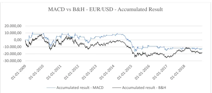
The MACD profitability, in EUR/USD, overcame B&H strategy by 6% of overall return, amounting to 5,737 USD, during the total time-period. Both strategies resulted in negative returns of 12% (12,276 USD) in MACD and 18% (18,012 USD) in B&H. Thus, even though the tool was not profitable, it enabled reduction of total losses to the trader.

With some minor exceptions, MACD outperformed the B&H strategy during the entire period studied, as it is possible to conclude on Figure 4.

Figure 4 - MACD vs B&H - EUR/USD (January 1st_{, 2009 – December 31}st_{, 2018)}

Source: Author

5.1.2. MACD vs B&H – JPY/USD

In JPY/USD, profitability was also higher for MACD, rounding 4%, amounting to 3,533 USD when compared to B&H strategy. Both MACD and B&H resulted in negative returns of 13,619 USD (14%) and 17,153 USD (17%), respectively. Again, MACD enabled the reduction of total losses to the trader.

In Figure 5 is possible to see that both strategies followed a similar accumulated profit pattern and surpassed each other several times during the total time-period.

-30.000,00 -20.000,00 -10.000,00 0,00 10.000,00 20.000,00

MACD vs B&H - EUR/USD - Accumulated Result

22

Figure 5 - MACD vs B&H - JPY/USD (January 1st_{, 2009 – December 31}st_{, 2018)}

Source: Author

5.1.3. MACD vs B&H – GBP/USD

Like in EUR/USD and JPY/USD, MACD profitability was higher than B&H. Still, in GBP/USD the tool returned slightly 1% (951 USD) above B&H. Gaining positions amounted to 31,959 USD and losing positions summed 43,661 USD, netting a total loss of 11,703 USD, 12%. B&H also underperformed and the result was a negative return of 12,654 USD (13%).

Figure 6 - MACD vs B&H - GBP/USD (January 1st_{, 2009 – December 31}st_{, 2018)}

Source: Author -40.000,00 -30.000,00 -20.000,00 -10.000,00 0,00 10.000,00 20.000,00 30.000,00

MACD vs B&H - JPY/USD - Accumulated Result

Accumulated result - MACD Accumulated result - B&H

-20.000,00 -15.000,00 -10.000,00 -5.000,00 0,00 5.000,00 10.000,00 15.000,00 20.000,00

MACD vs B&H - GBP/USD - Accumulated Result

23

5.1.4. MACD vs B&H – AUD/USD

The currency pair of AUD/USD was the one where MACD had the worst performance of all five currency pairs studied. Buy and Hold strategy resulted in a positive return around breakeven of 0.4% (406 USD) while MACD fall to a negative return of 8% (7,742 USD). In this case, Buy and Hold strategy was superior during the total length of the time-period studied, with the exception of the first four months of 2019 where no entry signal was marked by MACD and accumulated returns where negative for B&H.

Figure 7 - MACD vs B&H - AUD/USD (January 1st_{, 2009 – December 31}st_{, 2018)}

Source: Author

5.1.5. MACD vs B&H – CAD/USD

In CAD/USD, the tool was once again outperformed by the B&H strategy in 4%. The total closed positions with MACD returned a negative result of 14,780 USD, 15% of total initial capital, while B&H strategy, despite presenting a negative return of 10.489 (10%), showed better results.

Again, B&H strategy demonstrated to be the better option for the majority of period.

-40.000,00 -20.000,00 0,00 20.000,00 40.000,00 60.000,00 80.000,00

MACD vs B&H - AUD/USD - Accumulated Result

24

Figure 8 - MACD vs B&H - CAD/USD (January 1st_{, 2009 – December 31}st_{, 2018)}

Source: Author

5.2. RSI test results

The application of RSI on the dataset resulted in a total amount of signals between 57 and 81 observations. When comparing to MACD results, RSI market almost half of the positions. From the signals collected, between 7 and 11 open and closed investment positions were taken. The total signals marked by the tool, similarly to MACD, are distributed around 50% between long and short positions. However, the number profitable positions closed, tend to be higher for RSI.

In Table 4, one can observe that, similarly to MACD, non-profitable positions exceed profitable positions in terms of net gains or losses for almost all of the currency pairs (exception for AUD/USD that presented a positive return of 7%).

As presented before in MACD analysis, the profitability of RSI strategy is also in line with the market behaviour with negative returns presented by the B&H strategy with exception for AUD/USD.

Even though the overall returns of RSI strategy were negative, the tool was able to beat the returns of the B&H strategy for EUR/USD (+0.3%), JPY/USD (16%), and AUD/USD (+7%).

-30.000,00 -20.000,00 -10.000,00 0,00 10.000,00 20.000,00 30.000,00 40.000,00

MACD vs B&H - CAD/USD - Accumulated Result

25 For the remaining currency pairs, B&H strategy had better results: GBP/USD (-11%) and CAD/USD (-11%).

Description* EUR/USD JPY/USD GBP/USD AUD/USD CAD/USD

Total signals from tool 81 70 67 68 57

Long signals 43 (53%) 39 (56%) 39 (58%) 40 (59%) 29 (51%) Short signals 38 (47%) 31 (44%) 28 (42%) 28 (41%) 28 (49%)

Total closed positions 8 11 7 9 7

Closed gaining positions 4 (50%) 7 (64%) 4 (57%) 6 (67%) 3 (43%) Closed losing positions 4 (50%) 4 (36%) 3 (43%) 3 (33%) 4 (57%)

Initial Capital (RSI) 100,000 100,000 100,000 100,000 100,000

Trade gains 18,903 35,551 5,746 43,431 6,690

Trade losses (36,658) (36,886) (29,180) (36,108) (28,429) Final Capital (RSI) 82,245 98,665 76,566 107,323 78,261

Total gains/losses ($) (17,755) (1,335) (23,434) 7.323 (21,739)

Total gains/losses (%) -18% -1% -23% 7% -22%

Initial Capital Buy and Hold 100,000 100,000 100,000 100,000 100,000

Final Capital Buy and Hold 81,988 82,847 87,346 100,406 89.511 Total gains/losses B&H ($) (18,012) (17,153) (12,654) 406 (10,489)

Total gains/losses B&H (%) -18% -17% -13% 0.4% -10%

Profitability MACD vs B&H ($) 257 15,817 (10,780) 6,917 (11,250)

Profitability MACD vs B&H (%) 0.3% 16% -11% 7% -11% *Monetary amounts in USD Table 4 - RSI overall results (January 1st_{, 2009 - December 31}st_{, 2018)}

Source: Author

5.2.1. RSI vs B&H – EUR/USD

The application of the tool in EUR/USD currency pair resulted in a higher return than the B&H strategy by a scarce 0.3% (257 USD). Both strategies were not profitable as RSI net loss was 17,755 USD, 18%, and B&H also netting a total loss of 18%, 18,012 USD.

Just like in MACD, it is possible to observe in Figure 9 that both strategies followed a similar accumulated profit pattern. However, the tool was able to surpass B&H for several occasions during the total time-period.

26

Figure 9 - RSI vs B&H - EUR/USD (January 1st_{, 2009 – December 31}st_{, 2018)}

Source: Author

5.2.2. RSI vs B&H – JPY/USD

The JPY/USD was the currency pair where RSI performed better, achieving 16% (15,817 USD) more profitability than B&H. As B&H result was negative by 17,153 USD, 17%, the tool was able to return a net loss of only 1% (1,335 USD).

During the entire trading session, RSI was able to be superior to B&H regarding accumulated results, as one can conclude in Figure 10.

Figure 10 - RSI vs B&H - JPY/USD (January 1st_{, 2009 – December 31}st_{, 2018)}

Source: Author -30.000,00 -25.000,00 -20.000,00 -15.000,00 -10.000,00-5.000,00 0,00 5.000,00 10.000,00 15.000,00

RSI vs B&H - EUR/USD - Accumulated Result

Accumulated result - RSI Accumulated result - B&H

-40.000,00 -30.000,00 -20.000,00 -10.000,00 0,00 10.000,00 20.000,00 30.000,00 40.000,00

RSI vs B&H - JPY/USD - Accumulated Result

27

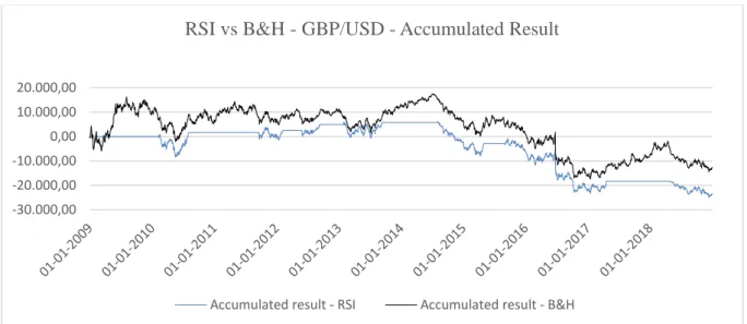
5.2.3. RSI vs B&H – GBP/USD

The profitability obtained from the tool when compared to B&H was inferior in 11% (10.780 USD). Despite the fact that both strategies resulted in negative returns, RSI total loss amounted to 23.434 USD (23%) while in B&H the net loss was 12.654 USD (13%). This currency pair had the worst performance along with CAD/USD, both outperformed by B&H in 11%.

During the total time-period is possible to see, in Figure 11, that the tool was never able to exceed B&H total accumulated return.

Figure 11 - RSI vs B&H - GBP/USD (January 1st_{, 2009 – December 31}st_{, 2018)}

Source: Author

5.2.4. RSI vs B&H – AUD/USD

The application of the tool to AUD/USD surpassed the B&H strategy by 7%, (6,917 USD). This was the only case, both in RSI and MACD, where the tool was able to generate positive returns to the initial capital of the trader by an amount of 7,323 USD (7%) while B&H strategy only resulted in a positive 0.4% return (406 USD). Despite of that fact, B&H performed better during the first seven years of the dataset only being surpassed by the tool in the last three years, as it possible to observe in Figure 12.

-30.000,00 -20.000,00 -10.000,00 0,00 10.000,00 20.000,00

RSI vs B&H - GBP/USD - Accumulated Result

28

Figure 12 - RSI vs B&H - AUD/USD (January 1st_{, 2009 – December 31}st_{, 2018)}

Source: Author

5.2.5. RSI vs B&H – CAD/USD

As stated above, CAD/USD was one of the worst performance of RSI, along with GBP/USD. The tool was outperformed by the B&H strategy in 11% (11,250 USD). The total loss for the trader was 21,739 USD (22%) with RSI while B&H net loss was 10,489 USD (10%).

During the total time-period is possible to see, in Figure 13, that the tool was never able to exceed B&H total accumulated return, with the exception of the first quarter of 2009.

Figure 13 - RSI vs B&H - CAD/USD (January 1st_{, 2009 – December 31}st_{, 2018)}

Source: Author -20.000,00 -10.000,000,00 10.000,00 20.000,00 30.000,00 40.000,00 50.000,00 60.000,00 70.000,00

RSI vs B&H - AUD/USD - Accumulated Result

Accumulated result - RSI Accumulated result - B&H

-40.000,00 -30.000,00 -20.000,00 -10.000,00 0,00 10.000,00 20.000,00 30.000,00 40.000,00

RSI vs B&H - CAD/USD - Accumulated Result

29

5.3. The shift in USD price

After analysing both indicators in all currency pairs and their respective B&H strategy performance, there is a cross-sectional phenomenon to all individual results. This situation is observable both through the figures of the cumulative results of each strategy and in the figures of the price evolution of each currency (Appendix II to VI). During the first half of the studied time-period (from 2009 to 2014) the accumulated results of each currency pair in both indicators were mostly positive when compared to the initial invested capital. However, approximately from the last semester of 2014 onwards, accumulated results started a downward trend and became negative until the end of the period studied, for all currency pairs of MACD and 4 out of 5 currency pairs in RSI (exception for RSI on AUD/USD which ended with a profitable return).

At the end of the first semester of 2014, cumulative results for both strategies were the following:

Indicator / Strategy EUR/USD JPY/USD GBP/USD AUD/USD CAD/USD

MACD ($) 8,401 (3,547) 8,476 8,777 1,107 % 8% -4% 8% 9% 1% RSI ($) (1,741) 10,075 5,746 24,651 (3,394) % -2% 10% 6% 25% -3% B&H ($) (2,134) (10,407) 17,097 34,302 14,400 % -2% -10% 17% 34% 14%

Table 5 - Profitability of MACD, RSI and B&H (June 30th_{, 2014)}

Source: Author

As at June 31st_{, 2014, four currency pairs were profitable with MACD and three where} profitable with RSI. The negative returns of the remaining currency pair where not so low as the results presented in the end of the total time-period.

The raise of USD price against the other currencies, beginning in 2014, was caused by the international markets expectations that U.S. Federal Reserves would increase interest rates in 2015. Thus, while investors had been investing in riskier markets searching for higher yields before that date, shifted their capital to the United States raising the demand for USD and consequently its price (Alice Ross, 2014).

30

5.4. Discussion of results

The results reached on the test of MACD tool are not conclusive as they point to divergent conclusions, depending on the currency pair studied. In fact, in three of the five currency pairs (EUR/USD, JPY/USD and GBP/USD) the performance of MACD was better that the B&H strategy. However, for the remaining currency pairs (AUD/USD and CAD/USD), MACD was outperformed by B&H strategy.

Another important result is that, in all cases, the tool was not able to obtain profitable returns as the investor ended his trading session with less capital than the one initially invested. This tendency also occurred when using the Buy and Hold strategy. Thus, the tool is not able to obtain profit from the up trending price variations without being exposed to higher losses when the market price decreases.

Thus, we cannot conclude positively on the hypothesis that the return of the investment positions based on the application of the MACD tool is higher than the return of the application of the B&H strategy.

In what concerns the performance of RSI tool, again, the results are inconclusive as they also point to divergent conclusions. When comparing the RSI tool with B&H strategy, three currency pairs presented better results for RSI (EUR/USD, JPY/USD and AUD/USD) and two currency pairs where favourable for B&H strategy (GBP/USD and CAD/USD).

The overall profitability of RSI when compared with the initial capital invested, was negative for all of the currency pairs except for AUD/USD. For that currency pair, the tool was able to achieve a profit for the investor. It is important to highlight that for this particularly currency pair, B&H strategy was also been able to generate a positive return for the investor, although much lower than RSI.

Thus, the hypothesis that the return of the investment positions based on the application of the RSI tool is higher than the return of the application of the B&H strategy cannot be confirmed.