An infinite servers queue systems with poisson and non poisson arrivals busy period simulation

(1)

M.A.M. Ferreira, M. Andrade. An infinite servers queue systems with poisson and non poisson arrivals busy period simulation. Emerging Issues in the Natural and Applied Sciences 2013; 3(1), 38-58. DOI: 10.7813/einas.2013/3-1/4

AN INFINITE SERVERS QUEUE SYSTEMS WITH

POISSON AND NON POISSON ARRIVALS

BUSY PERIOD SIMULATION

Prof. Dr. Manuel Alberto M. Ferreira, Prof. Dr. Marina Andrade Instituto Universitário de Lisboa (ISCTE-IUL),

BRU-IUL, Lisboa (PORTUGAL)

E-mails: manuel.ferreira@iscte.pt, marina.andrade@iscte.pt DOI: 10.7813/einas.2013/3-1/4

ABSTRACT

Many interesting parameters in queue theory study either have not theoretical results or, existing, are mathematically intractable what makes their utility very scarce. In this case a possible issue is to use simulation methods in order to get more useful results. In this paper this procedure is followed to learn something more about quantities of interest for those infinite servers queue systems, in particular about busy period parameters and probability distributions. A fortran program to simulate the operation of infinite servers’ queues is presented in this work. Poisson arrivals processes are considered but not only.

Key words: Infinite servers, queue, arrivals, simulation,

(2)

1. INTRODUCTION

The lack of theoretical results, often difficult to obtain, or its extreme complexity that makes its utility doubtful, leads to the search for numerical methods in the study of queue systems.

Through this work this is done with computational simulation for queue systems with infinite servers. The most famous and studied among these systems is the M / G / ∞ queue. For it a lot of results are known and result very clear and simple to use, see for instance (Carrillo, 1981), (Ferreira, 2002) and (Ferreira and Andrade, 2009, 2010, 2010a, 2010b, 2011, 2012).

One of the situations simulated here is related to the consideration of non-Poisson arrivals that is: with non-exponential inter-arrival times, for which there are no analytical results.

Other results collected are about the busy period1, for Poisson and non-Poisson arrivals. In fact any queue system has a sequence of busy periods and idle periods. A busy period followed by an idle period is a busy cycle. In the study of infinite servers systems, busy periods very useful information is, for instance, about the maximum number of customers served simultaneously in a busy period. If something is known about this quantity the system may be dimensioned as a finite servers queue. As there are not analytical results the simulation is one of the issues to study it.

In the next section, details about the FORTRAN program designed to perform the simulations and the experiences implemented are presented. The following section consists in the presentation of the results and the respective comments. The paper ends with a concluding notes section.

Much of this work is considered in (Ferreira and Andrade, 2013).

1

A busy period begins with the arrival of a customer to the system, being it empty, ends when a customer abandons the system, letting it empty, there being always at least one customer in the system.

(3)

2. THE SIMULATION

The simulations were executed using a FORTRAN program, see Appendix, with the following parts:

i) A main program, in FORTRAN language, called FILAESP, ii) A subroutine GERASER,

iii) A package SSPLIB, iv) A system function RAN.

The proceedings are as follows:

i) The sequential random generation of 25 000 arrivals

instants, being the inter- arrivals mean time = 0.99600 (a number very close to 1but not exactly 1 because of computational and accuracy reasons),

ii) The generation of 25 000 service times that is added to the

arrivals instants so obtaining the departure instants,

iii) The time ordering of the arrivals and departure instants,

through an ordering algorithm making correspond to each arrival 1 and to each departure -1,

iv) The generation, in fact, of the queue adding by order those

values 1 and -1, in correspondence with the instants at which they occur,

v) The processing of the information, in iv), in to obtain a) Data related to the state of the system2:

 Number of the visits to the assumed states,  Mean sojourn time in each one of those states.

b) Data related to the busy period:

 The maximum number of customers served simultaneously in a busy period,

 The total number of customers served in the busy period,  The length of the busy period.

2

The state of the system, in a given instant, is the number of customers that are being served in that instant.

(4)

The arrivals instant generation is performed in the program FILAESP. The service times in the GERASER subroutine. The arrivals and departures instants ordering are performed in the program FILAESP through the SSPLIB package. The queue construction and the information processing occur also in FILAESP.

In the arrivals and departures generation are used sequences of pseudo-random numbers supplied by the system function RAN. In general it is made RAN (E*J), being E constant in each experience and assuming J the values from 1 to 25 000. E was chosen to be an integer with four digits.

- To the arrivals process one or two sequences of pseudo-random numbers are needed as considering M, exponential inter-arrival times, or E2, Erlang with parameter 2 inter-arrival

times. In the first case it must be made an option for an integer with four digits, E, and in the second for two integers with four digits that will be designated by E and by F. The same happens with the service distribution, considering so G or G and H, as working with M or E2.

The experiences performed are described below, being the mean service time and = the traffic intensity.

- M / M / ∞

E = 7 528 F = 7 548

= 4 = 4.016

Number of observed busy periods: 208

- M / M / ∞

E = 7 529 F = 7 549

= 5 = 5.020

(5)

- M / E2 / ∞ E = 7 528 G = 7 552 H = 6 666 = 4 = 4.016

- M / E2 / ∞ E = 7 529 G = 6 552 H = 6 667 = 5 = 5.020

- E2 / E2 / ∞ E = 4 536 F = 4 537 G = 5 224 H = 6 225 = 4 = 4.016

- E2 / E2 / ∞ E = 4 538 F = 4 539 G = 5 228 H = 6 229 = 5 = 5.020

The mean service times considered, 4 and 5 were those for which a reasonable number of busy periods were obtained, among

(6)

the highest. In fact, increasing the mean service time the observed busy periods decrease very quickly.

Note that for the systems M / M / ∞ and M / E2 / ∞, for the same

values of the arrivals instants generated are identical.

3. THE OUTCOMES – ANALYSIS AND COMMENTS

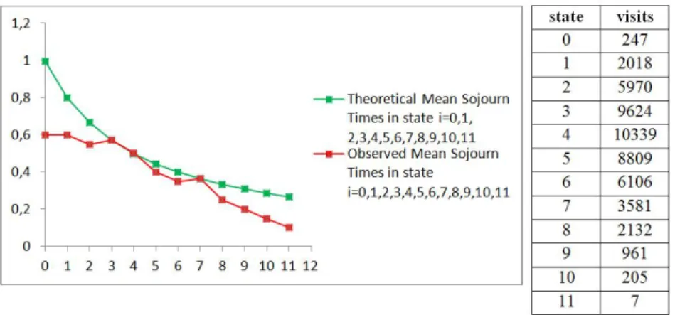
In Figure 1 and Figure 2 the graphics that represent the mean sojourn times in the various states3, for the M / M / ∞ system, considering ρ = 4.016 and ρ = 5.020, respectively, are presented. Beyond the observed mean values the theoretical values are also presented, see (Ramalhoto, 1983), given by

= , = 0, 1, 2, … (1).

In correspondence with the various states are also indicated the number of times that they were visited, in the right columns.

Fig. 1. Mean Sojourn Times, in seconds, theoretical and observed, for

the M / M / ∞ queue system in states i = 0, 1,…, 11, with ρ = 4.016.

3

The state of the system in a given instant is the number of costumers that are being served in that instant.

(7)

Fig. 2. Mean Sojourn Times, in seconds, theoretical and observed, for

the M / M / ∞ queue system in states i = 0, 1,…, 11, with ρ = 5.020.

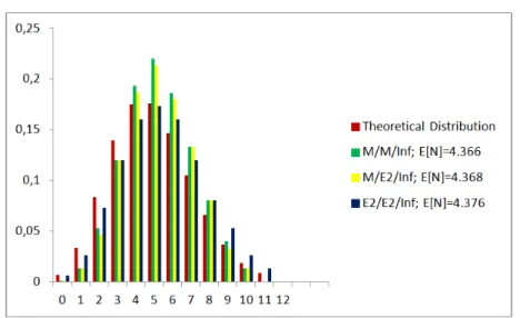
In Figure 3 and Figure 4 are shown the distributions obtained for the number of customers in the systems M / M / ∞, M / E2 / ∞ and E2

/ E2 / ∞ with ρ = 4.016 and ρ = 5.020, respectively. Together is also

presented the theoretical distribution, in equilibrium, for the systems M / M / ∞ and M / E2 / ∞, see (Tackács, 1962):

=

!, = 0, 1, 2, … (2), Obtained performing the direct computations for ρ = 4.016 and ρ = 5.020. E [N] is the mean number of customers in the system.

(8)

Fig. 3. Distribution of the Number of Customers in the System and Theoretical

Distribution for the Systems M / M / ∞, M / E2 / ∞ and E2 / E2 / ∞ with ρ = 4.016.

Fig. 4. Distribution of the Number of Customers in the System and Theoretical

(9)

These Figures suggest some similarity of behaviour among the empirical distributions and the theoretical distribution. Particularly, in the whole of them the mode is identical to the one of the theoretical distribution. But although for the systems M / M / ∞ and M / E2 / ∞

the empirical distributions are more concentrated around the mode, in comparison with the theoretical distribution, the opposite happens to the system E2 / E2 / ∞. And, surprisingly because for this system it

is not known the theoretical distribution, the empirical distributions obtained for E2 / E2 / ∞ seems closer to the theoretical distribution

than the ones of the other systems.

As for the differences observed between the systems M / M / ∞ and M / E2 / ∞, for the number of the customers in the system, the

adequate interpretation may be as follows: although the systems reach certainly the equilibrium, since the number of the simulated arrivals is quite large there is a strong presence of an initial transitory trend that must last a long time. Note, observing Figure 1 and Figure 2, that the mean sojourn times observed and theoretical, given by (1), for the system M / M / ∞ are quite close. This closeness is better for the states to which corresponds greater frequency.

In Figure 5 and Figure 6, about the maximum number of customers served simultaneously in the busy period, it is remarked great diversity in the distributions form. It is always observed a great frequency for the state 1. In the E2 / E2 / ∞ infinite systems it is

always the mode. Curiously, these systems being able to serve any number of customers, present, in these simulations, few customers being served simultaneously: never above the number 14, only assumed by the E2 / E2 / ∞ infinite systems. This fact is acceptable,

in terms of the theoretical distribution, since in the Poisson distribution the values greater than the mode, far away from it, are little probable. Note still that, excluding from this analysis the state 1, the distributions of maximum number of customers served simultaneously in the E2 / E2 / ∞ infinite systems busy period are

more scattered than those of the others. This is in accordance with the fact that, for the same number of arrivals, much more busy periods are observed for the E2 / E2 / ∞ infinite systems.

(10)

Fig. 5. Distribution of the Maximum Number of Customers Served Simultaneously in

a Busy Period for the Systems M / M / ∞, M / E2 / ∞ and E2 / E2 / ∞ with ρ = 4.016.

Fig. 6. Distribution of the Maximum Number of Customers Served Simultaneously in

a Busy Period for the Systems M / M / ∞, M / E2 / ∞ and E2 / E2 / ∞ with ρ = 5.020.

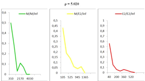
Figure 7 suggests a more and more smooth behaviour of the busy period lengths distribution frequency curve when going from M / M / ∞ system for the M / E2 / ∞ system and then for the E2 / E2 / ∞

(11)

system. The whole of them present a great frequency concentration for the lowest values of the busy period lengths but, in the case of M / M / ∞ system, the interval along which the observations spread has more than the double of the length of the other systems. Remember, a g a i n , t h a t f o r t h e M / M / ∞ s y s t e m m u c h

Fig. 7. Distribution of Observed Busy Period Lengths, in seconds, for the

Systems M / M / ∞, M / E2 / ∞ and E2 / E2 / ∞ with ρ = 4.016.

less busy periods are observed than for the M / E2 / ∞ system

and, for this one less than for the E2 / E2 / ∞ system. Then the curve

of frequencies for the M / M / ∞ system spreads along that interval with two deep valleys. The one of the M / E2 / ∞ system presents

also two valleys, but less deep, and in E2 / E2 / ∞ system practically

they are not observed. Note, also that those valleys occur for different values in the M / M / ∞ and M / E2 / ∞ systems.

Figure 8 suggests a greater similarity among the busy period lengths distributions of the various systems. Again it is observed a g r e a t c o n c e n t r a t i o n i n t h e l o w e s t v a l u e s ,

(12)

Fig. 8. Distribution of Observed Busy Period Lengths, in seconds, for the

Systems M / M / ∞, M / E2 / ∞ and E2 / E2 / ∞ with ρ = 5.020.

although lesser than in Figure 7. But now it is presented present one valley in each graphic. Still goes on observing a great disparity among the maximum values assumed by the busy period lengths.

It seems evident, either in Figure 7 or in Figure 8, a sharp observations lack in the intermediate values zone for the busy period lengths.

Note also that the Figures 7 and 8 are in accordance with the studies that point in order that the busy period length distribution of the M / G / ∞ system is right asymmetric and leptokurtic see (Ferreira and Ramalhoto, 1994).

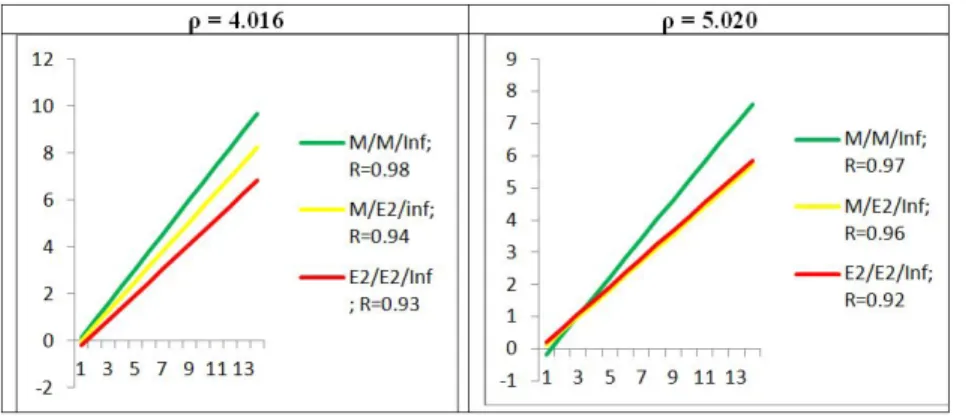
Call X and Y the maximum number of customers served simultaneously and the total number of served customers, respectively, in the busy period. Performing the regression of = ln on X, the results obtained are presented graphically in Figure 9 and the most interesting fact is, maybe, the similarity of the lines behaviour, for the various systems, for the two values of ρ considered. In fact, among the whole considered systems there is a great resemblance of the values of (the intercept) and

(13)

Fig. 9. Regression of Z over X, for the Systems M / M / ∞, M / E2 / ∞ and E2 / E2 / ∞ with ρ = 4.016 and ρ = 5.020. R is the Linear Correlation Coefficient.

the slope for the two values of ρ considered. Actually, it seems natural that the relation between Z and X does not depend on ρ. The values of ρ will only influence the values of Z and X that may occur and not the relation between them. Otherwise, will it be true that the differences observed in the values of and , for the various systems, not being too great, allow facing the hypothesis that the relation between Z and X is identical for those systems? Maybe yes if it is paid attention to the similarities observed in its behaviour: namely the ones related with the distribution of the number of customers in the various systems.

4. CONCLUDING NOTES

It is evident the great waste of these systems when looking to the maximum number of customers present simultaneously in the system.

It is uncontroversial, also, that there is a strong exponential relation between the maximum number of customers served simultaneously in a busy period and the total number of served customers. The question is if either it is always the same or how will it change either with the values of ρ or from system to system.

(14)

i) The great occurrence of busy periods with only one served

customer,

ii) The great amplitude of the interval at which happen the

values of the lengths of the busy periods, although with a great irregularity, and a great occurrence of low values. The results of these simulations seem to suggest also that the systems GI /G / ∞ may be quite well approximated by systems M / G / ∞, at least when the GI process possesses a regularity not very far from the one of the Poisson process.

REFERENCES

1. Andrade M.: A Note on Foundations of Probability. Journal of Mathematics and Technology, vol.. 1, No 1, pp 96-98, 2010.

2. Carrillo M. J.: Extensions of Palm’s Theorem: A Review. In Management Science, Vol. 37, No 6, pp. 739-744, 1991. 3. Ferreira M.A.M.: Simulação de variáveis aleatórias –

Método de Monte Carlo. Revista Portuguesa de Gestão, I

(III/IV), pp. 119-127. ISCTE, 1994.

4. Ferreira M.A.M.: Application of Ricatti Equation to the Busy

Period Study of the MG System. In Statistical Review,

1st Quadrimester, INE, pp. 23-28, 1998.

5. Ferreira M.A.M.: Computational Simulation of Infinite

Servers Systems. In Statistical Review, 3rd Quadrimester, INE, pp. 5-28, 1998a.

6. Ferreira M.A.M.: MG Queue Heavy-Traffic Situation Busy Period Length Distribution (Power and Pareto Service Distributions). In Statistical Review, 1st Quadrimester, INE, pp. 27-36, 2001.

7. Ferreira M.A.M.: The Exponentiality of the MG Queue Busy Period. In Actas das XII Jornadas Luso-Espanholas

de Gestão Científica, Volume VIII- Economia da Empresa e Matemática Aplicada. UBI, Covilhã, Portugal. pp. 267-272, 2002.

(15)

8. Ferreira M.A.M.: The MD Queue Busy Cycle Distribution. International Mathematical Forum, Vol. 9, No

2, pp. 81-87, 2014.

9. Ferreira M.A.M. and Andrade, M.: The Ties Between the

M/G/ Queue System Transient Behaviour and the Busy Period. In International Journal of Academic Research Vol.

1, No 1, pp. 84-92, 2009.

10. Ferreira M.A.M. and Andrade M.: Looking to a M/G/

system occupation through a Ricatti equation. In Journal of Mathematics and Technology, Vol. 1, No 2, pp. 58-62, 2010.

11. Ferreira M.A.M. and Andrade, M.: M/G/ System Transient Behavior with Time Origin at the Beginning of a Busy Period Mean and Variance. In Aplimat- Journal of Applied

Mathematics, Vol. 3, No 3, pp. 213-221, 2010a.

12. Ferreira M.A.M. and Andrade, M.: M/G/ Queue Busy Period Tail. In Journal of Mathematics and Technology, Vol. 1, No 3, 11-16, 2010b.

13. Ferreira M.A.M. and Andrade, M.: Fundaments of Theory

of Queues. International Journal of Academic Research,

Vol. 3, No 1, part II, pp. 427-429, 2011.

14. Ferreira M.A.M. and Andrade M.: Busy Period and Busy

Cycle Distributions and Parameters for a Particular M/G/oo queue system. American Journal of Mathematics and

Statistics, Vol. 2, No 2, pp. 10-15, 2012.

15. Ferreira M.A.M. and Andrade M.: Infinite Servers Queue

Systems Computational Simulation. In International

Conference APLIMAT, 12th, Bratislava: Slovak University of Technology, 2013.

16. Ferreira M.A.M. and Ramalhoto M.F.: Estudo dos

parâmetros básicos do Período de Ocupação da Fila de Espera MG. In A Estatística e o Futuro da Estatística. Actas do I Congresso Anual da S.P.E.. Edições Salamandra, Lisboa, 1994.

17. Ferreira M.A.M., Andrade, M. and Filipe, J. A.: The Ricatti Equation in the MG Busy Cycle Study. In Journal of

(16)

Mathematics, Statistics and Allied Fields Vol. 2, No 1, 2008.

18. Ferreira M.A.M., Andrade M. and Filipe J.A.: Networks of

Queues with Infinite Servers in Each Node Applied to the Management of a Two Echelons Repair System. In

China-USA Business Review Vol. 8, No 8, pp. 39-45 and 62, 2009.

19. Figueira J. and Ferreira M.A.M.: Representation of a

Pensions Fund by a Stochastic Network with Two Nodes: An Exercise. In Portuguese Revue of Financial Markets,

Vol. I, No 3, 1999.

20. Hershey J.C., Weiss E.N. and Morris A.C.: A Stochastic

Service Network Model with Application to Hospital Facilities. In Operations Research, Vol. 29, No 1, pp. 1-22,

1981.

21. Kelly F.P.: Reversibility and Stochastic Networks. New York: John Wiley and Sons, 1979.

22. Kendall and Stuart: The Advanced Theory of Statistics.

Distributions Theory. London. Charles Griffin and Co., Ltd.

4th Edition, 1979.

23. Kleinrock L.: Queueing Systems. Vol. I and Vol. II. Wiley- New York, 1985.

24. Metropolis N. and Ulan S.: The Monte Carlo Method. Journal of American Statistical Association, Vol. 44, No 247, pp. 335-341, 1949.

25. Murteira B.: Probabilidades e Estatística,. Vol. I. Editora McGraw-Hill de Portugal, Lda. Lisboa, 1979.

26. Ramalhoto M. F.: A Note on the Variance of the Busy

Period of the MG Systems. Centro de Estatística e

Aplicações, CEAUL, do INIC and IST. 1983.

27. Stadje W.: The Busy Period of the Queueing System

MG. In Journal of Applied Probability, Vol. 22, pp.

697-704, 1985.

28. Syski R.: Introduction to Congestion Theory in Telephone

Systems, Oliver and Boyd- London, 1960.

29. Syski R.: Introduction to Congestion Theory in Telephone

(17)

30. Tackács L.: An Introduction to Queueing Theory. Oxford University Press. New York, 1962.

APPENDIX PROGRAM FILAESP

C APAGUE 666 OU 555 CONFORME QUEIRA TEMPO INTERCHEGADAS C EXPONENCIAL OU ERLANG DE PARAMETRO 2

DIMENSION V(25000),Y1(25000),Y2(25000),TEPSER(25000) DIMENSION C(25000),AUX(50000),P(25000),N(50000),F(50000) DIMENSION Z(50000),VAL(50000),ARG(50000) DIMENSION NO(0:50000),T(0:25000),TM(0:25000) DIMENSION TTR(0:25000),TMR(0:25000) DIMENSION BUPE(0:25000),NA(0:25000)

WRITE(*,*)’O CODIGO DOS SERVICOS E: 0 PARA A PARETO, 1 PARA A’ WRITE(*,*)’EXPONENCIAL, 2 PARA A ERLANG, 3 PARA A LOGNORMAL,’ WRITE(*,*)’4 PARA A MISTURA DE EXPONENCIAIS COM RPARAMETRO,’ WRITE(*,*)’5 PARA A MISTURA DE ERLANG.’

WRITE(*,*)’ ’

WRITE(*,*)’ QUAL E O CODIGO DA DISTRIBUICAO DE SERVICO?’ READ(*,*) ICOD

WRITE(*,*)’ ’

WRITE(*,*)’ BOA SORTE NA VIAGEM AO MUNDO DA SIMULACAO ’ WRITE(*,*)’ ’ WRITE(*,*)’ ’ U=0.99600 DO 100 I=1,25000 555 V(I)=ALOG(RAN(E*I))*(-U/2.0) 666 V(I)=ALOG(RAN(E*I))*(-U/2.0)+ALOG(RAN(F*I))*(-U/2.0) 100 CONTINUE CALL GERASER(TEPSER) C(1)=V(1) Z(1)=C(1) F(1)=1 Z(25001)=V(1)+TEPSER(1) F(25001)=-1 DO 500 I=2,25000 C(I)=C(I-1)+V(I) P(I)=C(I)+TEPSER(I) Z(I)=C(I) F(I)=1 Z(I+25000)=P(I) F(I+25000)=-1

(18)

500 CONTINUE X=0.0 ICOL=1 IROW=50000 NDIM=50000 CALL ATSG(X,Z,F,AUX,IROW,ICOL,ARG,VAL,NDIM) N(1)=1 DO 600 I=2,50000 N(I)=N(I-1)+VAL(I) 600 CONTINUE MAX=1 DO 650 I=2,50000ESTRE DE 1998 IF (N(I).GE.MAX)MAX=N(I) 650 CONTINUE

WRITE(10,*)’ SIMULACAO FILA DE ESPERA M|G| ‘ DO 700 K=0,MAX

WRITE(10,*)’ TEMPOS DE RECORRENCIA DO ESTADO ‘,K J=1 NO(K)=0 T(K)=0.0 TM(K)=0.0 DO 660 I=1,49999 IF(N(I).EQ.K) THEN NO(K)=NO(K)+1 T(K)=T(K)+(ARG(I+1)-ARG(I)) J=J+1 ENDIF 660 CONTINUE DO 1000 J=1,NO(K)-1 TTR(K)=TTR(K) 1000 CONTINUE IF(NO(K).NE.0)TM(K)=T(K)/NO(K) IF(NO(K).GT.1)TMR(K)=TTR(K)/(NO(K)-1) IF(NO(K).EQ.1)TMR(K)=0 WRITE(10,*)’ESTADO’,K

WRITE(10,*)’NUMERO DE VISITAS =’,NO(K) WRITE(10,*)’TEMPO DE PERMANENCIA =’,T(K)

WRITE(10,*)’TEMPO MEDIO DE PERMANENCIA =’,TM(K) WRITE(10,*)’TEMPO TOTAL DE RECORRENCIA =’,TTR(K) WRITE(10,*)’TEMPO MEDIO DE RECORRENCIA =’,TMR(K) 700 CONTINUE TTBUPE=ARG(50000)-ARG(1)-T(0) NTBUPE=1+N0(0) TMBUPE=TTBUPE/NTBUPE TTIDP=T(0) NTIDP=NO(0)

(19)

TMIDP=TM(0)

WRITE(10,*)’NO TOTAL DE PERIODOS DE OCUPACAO =’,NTBUPE WRITE(10,*)’TEMPO TOTAL DE BUSY PERIOD =’,TTBUPE

WRITE(10,*)’TEMPO MEDIO DE BUSY PERIOD =’,TMBUPE

WRITE(10,*)’NO TOTAL DE PERIODOS DE DESOCUPACAO =’,NTIDP WRITE(10,*)’TEMPO TOTAL DE IDLE PERIOD =’,TTIDP

WRITE(10,*)’TEMPO MEDIO DE IDLE PERIOD =’,TMIDP BUPE(0)=0 NA(0)=1 NP=0 DO 5000 I=1,49999 IF(N(I).EQ.0) THEN NP=NP+1

WRITE(10,*)’BUSY PERIOD NUMERO’,NP NA(NP)=I NB=0 DO 4000 J=NA(NP-1),NA(NP)-1 IF(N(J+1).GT.N(J))NB=NB+1 4000 CONTINUE IF(NP.EQ.1)NB=NB+1

WRITE(10,*)’NUMERO DE CLIENTES ATENDIDOS=’,NB MAXI=1

DO 3900 J=NA(NP-1),NA(NP)

I IF(N(J).GE.MAXI) MAXI=N(J) 3900 CONTINUE

WRITE(10,*)’NUMERO MAXIMO DE CLIENTES ATENDIDOS SIMULTANEAMENTE=’,MAXI BUPE(NP)=ARG(I+1) RBUPE=BUPE(NP)-BUPE(NP-1)-ARG(I+1)+ARG(I) IF(NP.EQ.1)RBUPE=BUPE(1)-ARG(I+1)+ARG(I)-ARG(1) WRITE(10,*)’COMPRIMENTO=’,RBUPE ENDIF 5000 CONTINUE NP=NP+1

WRITE(10,*)’BUSY PERIOD NUMERO=’,NP NB=0

DO 4001 J=NA(NP-1),49999 IF(N(J+1).GT.N(J))NB=NB+1 4001 CONTINUE

IF(NP.EQ.1)NB=NB+1

WRITE(10,*)’NUMERO DE CLIENTES ATENDIDOS=’NB MA=1

DO 4002 J=NA(NP-1),50000 IF(N(J).GE.MA)MA=N(J) 4002 CONTINUE

(20)

WRITE(10,*)’NUMERO MAXIMO DE CLIENTES ATENDIDOS SIMULTANEAMENTE=’MA RBUPE=ARG(50000)-BUPE(NP-1) IF(NP.EQ.1)RBUPE=ARG(50000)-ARG(1) WRITE(10,*)’COMPRIMENTO= ’,RBUPE END SUBROUTINE GERASER (T) DIMENSION T(25000) ICOD=2 IF (ICOD.EQ.0) THEN

PRINT*, ‘INTRODUZA O VALOR DO COEFICINTE DE VARIACAO’ READ*,GAMA

ALFA=2*GAMA/(GAMA-1.0) RK=E*(GAMA+1.0)/(2*GAMA) ELSEIF (ICOD.EQ.4) THEN

PRINT*,’INTRODUZA O VALOR DO PARAMETRO DA MISTURA’ READ(*,*)RPARAMETRO ENDIF IX=35 IY=43 IIX=9 IJX=5 IKX=11 ILX=13 DO 10 I=1,250000 CALL RANDU(IX,IY,FL) IF(ICOD.EQ.O) THEN T(I)=RK/(1-FL)**(1.0/ALFA) ELSE IF (ICOD.EQ.1) THEN T(I)=-7.0*ALOG(RAN(G*I)) ELSE IF (ICOD.EQ.2) THEN

T(I)=-(4.0/2.0)*ALOG(RAN(G*I))-(4.0/2.0)*ALOG(RAN(H*I)) ELSE IF (ICOD.EQ.3) THEN

CALL RANDU(JX,IJY,YFFL) IJX=IJY

T(I)=EXP((-2*ALOG(YFFL))**(0.5)*COS(8*ATAN(1.0)*FL)) ELSE IF (ICOD.EQ.4) THEN

CALL RANDU (IKX,IKY,RFL) IKX=IKY

CALL RANDU (ILX,ILY,SFL) ILX=ILY

IF (FL.LE.RPARAMETRO) THEN

(21)

ELSE

T(I)=-(3.45/2.0)*(1.0/1.0-RPARAMETRO)*LOG(SFL) ENDIF

ELSE IF (ICOD.EQ.5) THEN CALL RANDU (IKX,IKY,RFL) IKX=IKY

CALL RANDU (ILX,ILY,SFL) ILX=ILY

CALL RANDU (IMX,IMY,TFL) IMX=IMY