Modelling and forecasting the UK tourism growth cycle in Algarve

(1)

Modelling and forecasting the UK tourism

growth cycle in Algarve

JORGE L.M. ANDRAZ

Centre for Advanced Studies in Economics and Econometrics (CASEE), Faculty of Economics, University of Algarve, Campus de Gambelas, 8005-139 Faro, Portugal.

PEDRO M.D.C.B. GOUVEIA

Escola Superior de Gestão, Hotelaria e Turismo (ESGHT) and Centre for Advanced Studies in Economics and Econometrics (CASEE), University of Algarve, Faro, Portugal.

PAULO M.M. RODRIGUES

Banco de Portugal, Lisbon, Faculty of Economics, Universidade Nova de Lisboa and Centre for Advanced Studies in Economics and Econometrics (CASEE), Faculty of Economics,

University of Algarve, Campus de Gambelas, 8005-139 Faro, Portugal. E-mail: prodrig@ualg.pt.

Over the past three decades, Portugal has developed a strong economic dependence on tourism, which has several implications for the country’s overall economic development. Tourism is an activity that is interrelated strongly with the economic system since Portugal as a whole and specific regions in particular rely on the performance of tourism for their economic activity. Moreover, because economic cycles affect tourism development, it is highly vulnerable to economic fluctuations. Most tourists who visit Portugal are from the European Union, especially Western Europe. Statistics are based on the number of overnight stays in hotel accommodation and other similar establishments. In 2005, the main source markets were the UK (30.7%), Germany (16.5%), Spain (11.5%), the Netherlands (6.8%), France (4.7%), Ireland (3.6%) and Italy (3.1%). These values show that the UK has the greatest share of visitors to Algarve. The purpose of this paper is to propose a modelling approach that best fits the tourism flow pattern in order to support forecasting. The paper contributes to our understanding of the relationship between economic cycles and tourism flows to Portugal (Algarve) and explores the potential of applying the diffusion index model proposed by Stock and Watson (1999, 2002) for tourism demand forecasting.

The authors thank Professor Stephen Wanhill for his useful comments and suggestions. Financial support from the Portuguese Science Foundation (Grant Reference PTDC/ECO/64595/2006) is gratefully acknowledged.

Andraz, Jorge Miguel Lopo Gonçalves; Gouveia, Pedro; Rodrigues, Paulo M. M.Modelling and Forecasting the UK Tourism Growth Cycle in Algarve, Tourism Economics, 15, 2, 323-338, 2009.

(2)

Keywords: diffusion index model; principal components; tourism

forecasting; Portugal

JEL classification: C51, C52, C53, L83

The service economy is a growing driving force, flourishing in most OECD countries. It represents a large share of economic activity and its importance is increasing. Tourism is a large, complex and fragmented industry and represents a key component of the service economy, constituting 30% of the international services trade in OECD economies. In terms of revenue, OECD countries generate about 70% of the world’s tourism activity. Although it has expanded dramatically over the past 30 years, the tourism industry looks set to continue expanding as societies become more mobile and prosperous.

Portugal is an example of a country with a strong economic dependence on tourism. This sector is responsible for about 8% of GDP and 10% of employment. The increasing number of tourists and tourism’s strategic importance in terms of revenue and employment, as well as in terms of direct and indirect effects on several other economic sectors, have led economic agents to adopt important dynamic measures in relation to supply. Portugal has been able to keep its international market share despite the growing number of competing markets that are once again attracting tourists to traditional destinations. In 2004, Portugal was ranked 19th among the main tourist destinations, having received over 11.6 million tourists, and 21st in terms of revenue, which generated €6.3 billion.

The sector’s strategic importance is well recognized by the leading authorities in Portugal. According to the State Budget for 2007, the Tourism National Strategic Plan looks to develop measures to increase the quality of and diversify tourism demand in Portugal in order to capture tourist flows well above the European average and to increase the average revenue per tourist. To achieve this, the government intends to strengthen the tourism sector by stimulating the strategic convergence and the efficiency of promotional investments in target foreign markets.

This dependency generates several issues for the country’s overall economic development. Tourism is an activity that is interrelated strongly with the economic system since Portugal and specific regions in particular rely on tourism for their economic stability. However, economic cycles impact on the development of the tourism industry, which is prone to unstable economic fluctuations.

The majority of tourists that visit Portugal are from western EU countries. Statistics are based on the number of overnight stays in hotel accommodation and other similar establishments. In 2005, the main source markets were the UK (30.7%), Germany (16.5%), Spain (11.5%), the Netherlands (6.8%), France (4.7%), Ireland (3.6%) and Italy (3.1%). These values show that the UK holds the strongest share of visitors coming to Algarve.

The purpose of this paper is to propose a modelling approach that best fits the tourism flow pattern in order to support forecasting decisions. Recent literature has shown that the lack of parsimony may be an important deter-minant of forecast failure. Hence, factor models will play an important role in

(3)

this context, particularly because they enable all information, represented in a large set of variables, to be captured by a small number of common factors. As pointed out by Ferreira et al (2005), at least two distinct strands of literature adopt this method: (i) dynamic factor models (see inter alia Sargent and Sims, 1977; Engle and Watson, 1981; Geweke and Singleton, 1981; Stock and Watson, 1989, 1998; Quah and Sargent, 1993; and Kim and Nelson, 1998); and (ii) the diffusion index models (see, for instance, Connor and Korajczyk, 1993; Forni and Reichlin, 1996, 1998; Geweke and Zhou, 1996; and Stock and Watson, 1998, 2002). The former represents studies that look to estimate unobservable common factors among some macroeconomic variables, while the latter use principal components (PCs) to estimate the common factors. For the purpose of empirical analysis, we consider the number of overnight stays in hotel accommodation and similar establishments by tourists from the UK in Algarve, one of the Portuguese regions where dependence on tourism is quite evident.

This paper applies the diffusion index model, proposed by Stock and Watson (1999, 2002), to forecast tourism demand. Stock and Watson (1999, 2002) have shown that the information contained in a large set of variables can be summarized through the use of dynamic factor models, where a small number of unobserved common factors may capture co-movements across series. The diffusion index model proposed by Stock and Watson (1999, 2002) has been applied successfully in the forecasting of macroeconomic time series (see, inter alia, Stock and Watson, 1999, 2002; Angelini et al, 2001; Marcelino et al, 2003; Shintani, 2004; and Heij et al, 2006) and it has been shown to outperform traditional time series models in terms of forecasts. Recently, Breitung and Eickmeier (2005) have also pointed out that factor models are more advantageous than other models since (i) they can cope with many variables without running into problems of scarce degrees of freedom; (ii) idiosyncratic movements which possibly include measurement errors and local shocks can be eliminated; (iii) they remain agnostic about the structure of the economy; and (iv) they do not need to rely on overly tight assumptions, as is sometimes the case in structural models.

The paper is organized as follows. The next section describes briefly the data considered; the subsequent section introduces the diffusion index forecast model methodology; we then describe the construction of the models used in the forecasting exercise and present the results of the forecast study; and, finally, we present our conclusions.

The data

For the purposes of empirical analysis, we consider the number of overnight stays in hotel accommodation and similar establishments in Algarve by UK tourists. The sample period considered is from January 1987 to December 2005. The data are taken from statistics published by the Portuguese Office for National Statistics. Following Stock and Watson (1998), we need to ensure that the series are stationary. Thus, the transformation of the variables that were considered is such that it induces stationarity.

(4)

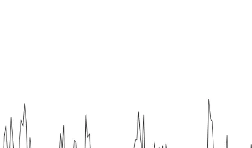
Figure 1. Number of overnight stays of British tourists.

Figure 2. Mean annual growth rate of overnight stays of British tourists.

0 100,000 200,000 300,000 400,000 500,000 600,000 700,000 800,000

Jan-89Jan-90 Jan-91Jan-92 Jan-93Jan-94 Jan-95 Jan-96 Jan-97Jan-98Jan-99 Jan-00Jan-01 Jan-02 Jan-03Jan-04 Jan-05

–30% –20% –10% 0% 10% 20% 30%

(5)

for Algarve used in this study. Specifically, the objective will be to forecast the transformed series presented in Figure 2, that is, the mean annual growth rate. Figure 1 depicts clearly the strong and slow changing seasonal pattern, which is characteristic of this series. Figure 2 presents the mean annual growth rate of the number of overnight stays of British tourists, which is the variable that will be analysed in this study.

The diffusion index forecast model methodology

The first step when building a tourism demand forecast model based on diffusion index models is related to the analysis between tourism demand and economic variables synchronization. The PC approach is intended to identify and explore the existing lags in the behaviour of the main macroeconomic variables and their effects on the level of tourism demand. Within this frame-work, we look to identify the factors that may be considered as coincident, lagging or leading indicators of the tourism demand flows; for details on this type of analysis, see Gouveia and Rodrigues (2005).

Identification of principal components

We consider a set of N variables x_t*_{, with t = 1,2,...,T, represented as the sum}

of two mutually orthogonal unobservable components: the common r-dimen-sional component F_t and the idiosyncratic N-dimensional component ε_t; that is,

x*_t₌Λ_F

t + εt, (1)

where xt* = [x*1t,...,x*Nt]′ is an N × 1 vector, Λ represents the N × r dimensional

matrix of factor loadings relating to the common factors of the observed series and Ft = [f1,…, fr]′ is an r × 1 vector of common factors. The estimated factors

are: X^ Λ ^ F = ––– , N

where ^Λ is equal to N½_{times the eigenvectors of X}′_X.

The main advantage of (1) is that it allows for the estimation of factors by PCs. Stock and Watson (1998) show that factors estimated by PCs are consistent as the number of variables increases (that is, tends to infinity), even for a fixed time period of the series, which is an interesting characteristic for empirical applications.

In this paper, the variable xt* is computed as:

1 11

x*t = –– Σ [ln(xt–s) – ln(xt–12–s)], (2)

12 s=0

which represents the mean annual growth rate of xt. The objective of this

transformation is to eliminate the seasonal component and to reduce the effect of short-run movement. For the UK confidence indicators, no transformation is applied since these variables take positive and negative values and present reduced variability in the short run.

(6)

Factor selection

The selection of the PCs to be included in the forecasting model is based on the maximum value of the coefficient of determination obtained from separate regressions between the tourism demand proxy and each identified factor lagged up to h periods (with h = 1,...,hmax, where hmax represents the maximum

forecasting period). In this way, the recursive nature of the forecasting process and the inclusion of the factors with the highest forecasting power is considered for each time horizon, h.

Estimation of the forecast model

For the purpose of forecasting, we consider the following model: y_t = µ₀ + Σp i=1 αiyt–i + k Σ v=1 qv Σ j=1 αvj ^ f_v,t–h–j + e_t , (3)

where k is the number of factors and p and q_v represent the maximum lag order of autoregressive and factor components, respectively.

The forecasts can be obtained from the expression:

^ y_t+ht = ^ µ0 + p Σ i=1 ^ αiyt–i + k Σ v=1 qv Σ j=1 ^ αvj ^ f_v,t–j . (4)

In this model, y_t represents the mean annual growth rate of the number of overnight stays in hotel accommodation and similar establishments by British tourists, and is computed following (2).

The reasons for including the h order lag in the model are twofold. First, it allows us to explore the potential lag between the behaviour of the economic variables and the evolution of tourism demand and, second, omitting such lags would require the forecasting of both the behaviour of the dependent variable and the set of factors used as explanatory variables.

The forecasting models are re-estimated recursively over this forecasting period. In other words, the appropriate PC lags and autoregressive orders are re-specified recursively during the forecast period. Furthermore, to guarantee parsimonious models, we consider the most significant order of the autoregressive components by excluding the non-significant components at a 5% significance level and controlling for autocorrelation in the residuals (see Rodrigues and Gouveia, 2004).

Measuring forecast performance

To evaluate forecast accuracy, we consider the use of the last m sample observations to evaluate h step-ahead forecasts generated from models fitted to the first (T – m) observations. Although many measures of forecast accuracy are available, we follow much of the literature in basing our evaluation on the root mean squared prediction error (RMSPE), defined as:

1 m

RMSPE(h) = ––––––––– Σ (_y^

T+jT+j–h – yT+j) 2_,

(7)

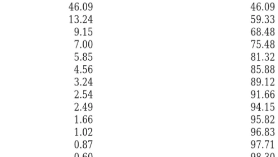
Table 1. Principal components.

Factor Percentage of variance Explained accumulated explained by each factor percentage of variance

F1 46.09 46.09 F2 13.24 59.33 F3 9.15 68.48 F4 7.00 75.48 F5 5.85 81.32 F6 4.56 85.88 F7 3.24 89.12 F8 2.54 91.66 F9 2.49 94.15 F10 1.66 95.82 F11 1.02 96.83 F12 0.87 97.71 F13 0.60 98.30 F14 0.48 98.79 F15 0.39 99.17 where _y^

T+jT+j–h is the h step-ahead forecast made for period (T + j) based on

data available at (T + j – h). Results are computed for horizons h = 1,...,hmax,

where hmax is the maximum forecast horizon.

Empirical study

Diagnostic results

For purposes of empirical analysis, we consider a set of 50% of the variables with the highest performance in terms of the coefficient of determination obtained from regressing the tourism demand proxy on each variable. From the 120 original economic variables, we selected the best 60 variables using this indicator. However, the selection of the initial data set is still an issue that deserves further research development.

From the set of the 60 economic variables selected, 15 PCs were extracted, corresponding to 99.17% of total variance. The percentage of variance explained by each factor is presented in Table 1.

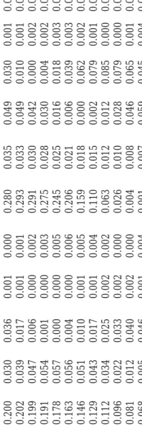
It is noticeable that F1, F2 and F3 are the three components that explain the largest proportion of the variance to a total of 68.48%. The next step of the analysis is related to the selection of the PCs. Table 2 presents the coefficients of determination obtained from regressing the tourism demand proxy on each factor, representing a total of 15 regressions, for different lagging periods and considering the best 50% variables (we also considered the analysis using the 75% variables, but the results did not show any qualitative differences).

In order to select the set of factors to include in the model, 15 factors were analysed, although at the forecast level only a maximum of 6 factors was considered for each forecast horizon. Table 3 allows us to rank the models and

(8)

T

able 2.

Goodness of fit of the factors in explaining UK tourism demand (50% best variables).

Factor lag F1 F2 F3 F4 F5 F6 F7 F8 F9 F10 F11 F12 F13 F14 F15 1 0.017 0.207 0.001 0.200 0.030 0.036 0.001 0.000 0.280 0.035 0.049 0.030 0.001 0.053 0.001 2 0.045 0.196 0.000 0.202 0.039 0.017 0.001 0.001 0.293 0.033 0.049 0.010 0.001 0.063 0.000 3 0.087 0.175 0.001 0.199 0.047 0.006 0.000 0.002 0.291 0.030 0.042 0.000 0.002 0.067 0.000 4 0.140 0.146 0.004 0.191 0.054 0.001 0.000 0.003 0.275 0.028 0.030 0.004 0.002 0.063 0.002 5 0.203 0.112 0.011 0.178 0.057 0.000 0.000 0.005 0.245 0.025 0.016 0.018 0.003 0.052 0.004 6 0.268 0.077 0.022 0.163 0.056 0.004 0.000 0.006 0.206 0.021 0.006 0.039 0.003 0.040 0.008 7 0.332 0.045 0.038 0.146 0.051 0.010 0.001 0.005 0.159 0.018 0.000 0.062 0.002 0.027 0.012 8 0.389 0.020 0.060 0.129 0.043 0.017 0.001 0.004 0.110 0.015 0.002 0.079 0.001 0.015 0.017 9 0.435 0.005 0.087 0.112 0.034 0.025 0.002 0.002 0.063 0.012 0.012 0.085 0.000 0.006 0.021 10 0.468 0.000 0.120 0.096 0.022 0.033 0.002 0.000 0.026 0.010 0.028 0.079 0.000 0.001 0.024 11 0.475 0.006 0.156 0.081 0.012 0.040 0.002 0.000 0.004 0.008 0.046 0.065 0.001 0.001 0.025 12 0.456 0.022 0.192 0.068 0.005 0.046 0.001 0.004 0.001 0.007 0.059 0.045 0.004 0.006 0.020 Mean 0.276 0.084 0.058 0.147 0.037 0.020 0.001 0.003 0.163 0.020 0.028 0.043 0.002 0.033 0.011

(9)

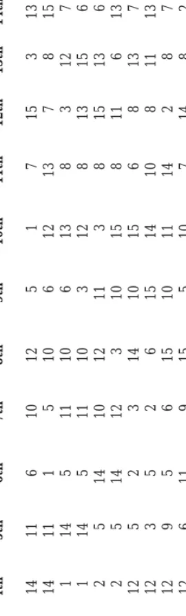
T able 3. Factor hierarchy . Factor lag 1st 2nd 3rd 4th 5th 6th 7th 8th 9th 10th 11th 12th 13th 14th 15th 1 9 2 4 14 11 6 1 0 1 2 5 1 7 15 3 1 3 8 2 9 4 2 14 11 1 5 10 6 1 2 1 3 7 8 1 5 3 3 9 4 2 1 1 4 5 11 10 6 1 3 8 3 1 2 7 15 4 9 4 2 1 1 4 5 11 10 3 1 2 8 13 15 6 7 5 9 1 4 2 5 1 4 10 12 11 3 8 15 13 6 7 6 1 94 25 1 4 1 2 3 1 0 1 5 8 1 1 6 1 3 7 7 1 9 4 12 5 2 3 1 4 1 0 1 5 6 8 1 3 7 11 8 1 4 9 12 3 5 2 6 15 14 10 8 1 1 1 3 7 9 1 4 3 12 9 5 6 1 5 1 0 1 1 1 4 2 8 7 13 10 1 3 4 1 2 6 1 1 9 1 5 5 10 7 1 4 8 2 1 3 11 1 3 4 1 2 1 1 6 15 5 1 0 2 9 7 13 14 8 12 1 3 4 1 1 6 1 2 2 1 5 1 0 1 4 5 13 8 7 9

(10)

help select the factors used in the forecasting exercise. It reveals that F1, F2 and F9 are ranked in the first positions for different time lags and therefore they present the largest explanatory power. Nevertheless, F9 explains only 2.49% of the variance of the selected set of variables.

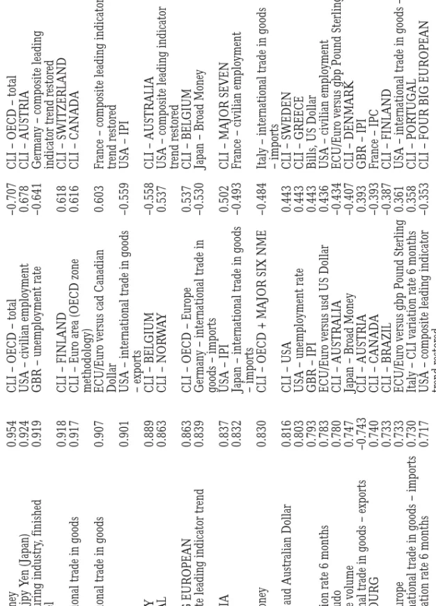
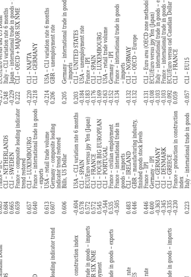
Regarding the selected components, while the first component essentially is influenced by USA Broad Money, ECU/Euro versus Japanese Yen exchange rates and some other exchange rate variables, reflecting also the European economic cycle, the second factor is influenced mostly by the performance of the USA. These results allow us to conclude that tourism demand growth is influenced, firstly and mainly by the change of relative prices (price sensitivity) and, secondly, by the change in the dynamics of economic activity, represented in terms of the effects on income. The behaviour of the first and second components reflects the adjustment period (lag) between the evolution of the economic variables and the growth of tourism demand, which allows for the use of these components as leading indicators of the tourism activity cycle. On the other hand, the 9th PC may be used as a coincident indicator of the pro-and anti-cyclical behaviour of the components. The factor loadings for the selected PCs are presented in a comprehensive manner in Table 4.

Forecasting study

Comparison models

In order to evaluate the quality of the forecasts obtained from the index models, we compare these with forecasts obtained from models used frequently in the literature, namely, the autoregressive moving average (ARMA) model and the pure autoregressive (AR) model.

The ARMA(p,q) model includes both autoregressive and moving average terms: yt = µ0 + p Σ i=1 φiyt–i + q Σ j=1 θj ut–j + ut , (5)

where p and q are the lag orders of the autoregressive and moving average components, respectively; whereas the AR(p) model results from (5) by considering q = 0. For more details on these models see, inter alia, Hamilton (1994).

Forecast design

We study the effects that the number of factors considered in the model have on forecasting accuracy. We consider k = 1,...,6 (where k represents the number of factors in the model). The lag orders of the factor and autoregressive components are based on the follow-up elimination of insignificant regressors. In this analysis, we consider several model specifications. We chose a maximum value for the PC and autoregressive lag order which was defined as [p_max(PC)] and [p_max(AR)], respectively, lying between 1 and 4. On the other hand, the number of PCs in model k can lie between 1 and 6. To analyse the quality of the forecasts, we use the RMSPE, with m = 6. All forecasting models are re-estimated recursively over this forecasting period. In addition, models that

(11)

require specification of the appropriate PC lags and autoregressive orders are also re-specified recursively during the forecast period. The PCs introduced in the diffusion index model are chosen by considering the results in Table 2.

Forecast results

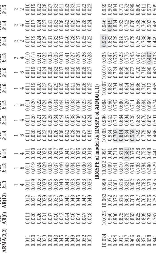
The forecast results are presented in Table 5. The upper part presents the RMSPE using different specifications of the ARMA and the diffusion index model for different horizons. The bottom part compares the performance of the different models with the ARMA(1,1) model by considering the ratio of their RMSPEs. Note that the ARMA(1,1) model is used frequently in the literature as the benchmark model.

From Table 5, we observe that, on average, all diffusion index models outperform the ARMA(1,1) model. Moreover, this superiority is confirmed by analysis of the comparative performance on a month-to-month basis. In fact, almost all diffusion index models outperform the ARMA(1,1) model as the ratios of the corresponding RMSPEs are below unity. The only exceptions are models M6, M8, M11 and M12 for h = 1.

Interestingly, out of the two ARMA models and the two AR models considered, the AR(12) seems to display the best forecast performance for the generality of the forecast horizons considered. Moreover, when comparing the results of the ARMA models with those of the diffusion index models, we observe that the worse performing diffusion index model at each forecast horizon (h = 1,…,12) in terms of RMSPE is very similar to the results of the best performing ARMA model, the AR(12), exceeding it marginally in a few cases only.

The analysis clarifies the superiority of the diffusion index models for all forecast horizons since, as can be observed from the highlighted values, the longer the forecast horizon, the greater is the difference between the ARMA(1,1) and the diffusion index models. This may be interpreted as positive evidence towards the choice of diffusion index models for long-term forecasting purposes. For the diffusion index models, the best performance can be observed for M8, M7 and M18.

Conclusion

This paper provides a pioneering approach in forecasting tourism demand, representing an improvement in forecasting performance. We use the depend-ence between economic and tourism growth cycles to determine our forecasts. We use the diffusion index model proposed by Stock and Watson (1998, 2002) which allows the information contained in a large number of variables to be summarized properly using dynamic factor models, where a small number of unobserved common factors capture co-movements across different series.

The analysis shows that tourism demand growth is influenced mainly by both exchange rate variables and the performance of the US economy. The superiority of the diffusion index model for forecasting purposes is observed when compared with traditional models such as ARMA and AR models. The analysis confirms the superiority for all forecast horizons. Specifically, the longer the forecast

(12)

T able 4. Factor loadings. Variable F 1 V ariable F2 V ariable F9

USA – Broad Money

0.954

CLI – OECD – total

–0.707

–0.456

ECU/Euro versus jpy

Y

en (Japan)

0.924

USA – civilian employment

0.678 CLI – AUSTRIA –0.453 GBR – manufacturing industry , finished 0.919 GBR – unemployment rate –0.641

Germany – composite leading

0.334

goods stocks, level

indicator trend restored

CLI – SP AIN 0.918 CLI – FINLAND 0.618 CLI – SWITZERLAND 0.321

France – international trade in goods

0.917

CLI – Euro area (OECD zone

0.616

CLI – CANADA

–0.301

– exports

methodology)

0.907

ECU/Euro versus cad

Canadian

0.603

France – composite leading indicator

–0.297 – imports Dollar trend restored CLI – FRANCE 0.901

USA – international trade in goods

–0.559 USA – IPI –0.222 – exports CLI – GERMANY 0.889 CLI – BELGIUM –0.558 CLI – AUSTRALIA 0.219 CLI – POR TUGAL 0.863 CLI – NOR W A Y 0.537

USA – composite leading indicator

0.216

trend restored

CLI – FOUR BIG EUROPEAN

0.863

CLI – OECD – Europe

0.537

CLI – BELGIUM

–0.214

France – composite leading indicator trend

0.839

Germany – international trade in

–0.530

Japan – Broad Money

0.212 restored goods – imports CLI – AUSTRALIA 0.837 USA – IPI 0.502

CLI – MAJOR SEVEN

–0.211

CLI – IRELAND

0.832

Japan – international trade in goods

–0.493

France – civilian employment

–0.207

– imports

0.830

CLI – OECD + MAJOR SIX NME

–0.484

Italy – international trade in goods

–0.191

– imports

ECU/Euro versus aud

Australian Dollar 0.816 CLI – USA 0.443 CLI – SWEDEN –0.174 CLI – GREECE 0.803

USA – unemployment rate

0.443 CLI – GREECE –0.169 France – IPC 0.793 GBR – IPI 0.443 Bills, US Dollar 0.160

Italy – CLI variation rate 6 months

0.783

ECU/Euro versus usd

US Dollar

0.436

0.160

Pound versus Escudo

0.780 CLI – AUSTRALIA –0.434 ECU/Euro versus gbp Pound Sterling –0.157

USA – retail trade volume

0.747

–0.407

CLI – DENMARK

–0.145

Italy – international trade in goods – exports

–0.743 CLI – AUSTRIA 0.393 GBR – IPI –0.135 CLI – LUXEMBOURG 0.740 CLI – CANADA –0.393 France – IPC –0.133 CLI – NOR W A Y 0.733 CLI – BRAZIL –0.387 CLI – FINLAND –0.110

0.733

ECU/Euro versus gbp

Pound Sterling

0.361

USA – international trade in goods – exports

0.109

Germany – international trade in goods – imports

0.730

0.358

CLI – POR

TUGAL

–0.101

USA – CLI – variation rate 6 months

0.717

USA – composite leading indicator

–0.353

–0.098

trend restored

CLI – Euro area (OECD zone methodology)

0.715

CLI – MAJOR SEVEN

0.353

CLI – IRELAND

0.089

USA – composite leading indicator trend

0.713

–0.351

Pound versus Escudo

–0.088

restored

– exports

ECU/Euro versus usd

US Dollar

0.698

CLI – NAFT

A

0.302

USA – Broad Money

–0.084

CLI – BRAZIL

0.695

Pound versus Escudo

0.278

CLI – BRAZIL

(13)

T

able 4.

Factor loadings (cont).

V ariable F1 V ariable F2 V ariable F9

ECU/Euro versus cad

Canadian Dollar

0.685

France – IPC

–0.273

ECU/Euro versus usd

US Dollar –0.075 CLI – NETHERLANDS 0.684 CLI – NETHERLANDS 0.248

0.072

Germany – IPI

0.665

CLI – SWEDEN

–0.229

Japan – international trade in goods – imports

0.067

Bills, US Dollar

0.659

France – composite leading indicator

0.222

0.066 trend restored CLI – FINLAND 0.657 CLI – LUXEMBOURG –0.220 CLI – NAFT A –0.066 CLI – SWITZERLAND 0.640

–0.218 CLI – GERMANY –0.063 – exports GBR – IPI 0.613

–0.214

USA – CLI variation rate 6 months

–0.057

Germany – composite leading indicator trend

0.607

Germany – composite leading

0.206

GBR – unemployment rate

0.055

restored

indicator trend restored

CLI – NAFT

A

0.606

Bills, US Dollar

0.205

Germany – international trade in goods

–0.055

– imports

France – production in construction index

–0.604

USA – CLI variation rate 6 months

0.203 CLI – UNITED ST A TES 0.051 CLI – DENMARK 0.578 CLI – SP AIN –0.184

0.051

Japan – international trade in goods – imports

0.572

ECU/Euro versus jpy

Y

en (Japan)

–0.183

France – IPI

–0.049

0.572 CLI – FRANCE –0.176 CLI – SP AIN –0.048

0.545

–0.169 CLI – LUXEMBOURG –0.047 CLI – AUSTRIA –0.544 CLI – POR TUGAL –0.163

–0.045

USA – international trade in goods – exports

0.535

–0.152

Germany – IPI

–0.041

CLI – CANADA

–0.505

France – international trade in

–0.134

–0.039 goods – imports – imports GBR – unemployment rate 0.483 CLI – IRELAND –0.132 CLI – NOR W A Y –0.031 CLI – UNITED ST A TES 0.446 GBR – manufacturing industry , –0.132

–0.031

finished goods stock levels

0.446

France – IPI

–0.131

CLI – Euro area (OECD zone methodology)

0.031

USA – IPI

0.400

Germany – IPI

–0.108

ECU/Euro versus jpy Y

en (Japan) –0.031 CLI – SWEDEN –0.363 CLI – GERMANY –0.103

Italy – international trade in goods – exports

0.029

CLI – EU15

–0.345

CLI – DENMARK

–0.103

France – international trade in goods – exports

0.018

Italy – international trade in goods – imports

–0.335

CLI – GREECE

–0.092

ECU/Euro versus cad

Canadian Dollar

0.014

France – IPI

–0.230

France – production in construction

0.059

CLI – FRANCE

–0.010

index

CLI – MAJOR SEVEN

0.223

–0.057 CLI – EU15 0.010 – imports CLI – BELGIUM 0.185 CLI – EU15 –0.051

ECU/Euro versus aud

Australian Dollar 0.007 ECU/Euro versus gbp Pound Sterling 0.141 CLI – SWITZERLAND 0.047

France – production in construction index

–0.002

0.100

ECU/Euro versus aud

Australian

–0.033

GBR – manufacturing industry finished

0.002

Dollar

goods stock levels

0.069

USA – Broad Money

0.005

CLI – NETHERLANDS

(14)

T

able 5.

Forecasting results.

ARMA models

Dif

fusion index models

h M1 M2 M3 M4 M5 M6 M7 M8 M9 M10 M11 M12 M13 M14 M15 M16 M17 M18 ARMA(1,1) ARMA(2,2) AR(6) AR(12) k =3 k =3 k =4 k =4 k =5 k =5 k =6 k =6 k =3 k =4 k =4 k =5 k =5 k =6 PC order 11 1 1 1 1 1 1 22 2 2 2 2 AR order 46 4 6 4 6 4 6 42 4 2 4 4 1 0.011 0.011 0.011 0.012 0.011 0.011 0.011 0.011 0.011 0.011 0.011 0.011 0.010 0.010 0.010 0.010 0.011 0.011 2 0.021 0.020 0.020 0.021 0.019 0.019 0.020 0.020 0.020 0.020 0.019 0.019 0.018 0.019 0.017 0.019 0.019 0.020 3 0.029 0.027 0.026 0.025 0.025 0.024 0.021 0.020 0.021 0.022 0.020 0.021 0.021 0.024 0.024 0.023 0.024 0.021 4 0.036 0.033 0.031 0.029 0.029 0.029 0.022 0.022 0.024 0.024 0.023 0.024 0.022 0.029 0.027 0.028 0.027 0.025 5 0.042 0.039 0.037 0.034 0.035 0.035 0.024 0.025 0.029 0.030 0.027 0.028 0.033 0.031 0.031 0.027 0.029 0.025 6 0.047 0.043 0.040 0.037 0.038 0.037 0.027 0.026 0.034 0.034 0.029 0.032 0.035 0.032 0.032 0.033 0.034 0.027 7 0.051 0.045 0.042 0.039 0.040 0.040 0.038 0.038 0.044 0.044 0.035 0.037 0.038 0.037 0.038 0.041 0.043 0.030 8 0.055 0.047 0.044 0.041 0.043 0.043 0.041 0.042 0.037 0.037 0.040 0.039 0.041 0.040 0.042 0.033 0.032 0.032 9 0.057 0.049 0.046 0.043 0.033 0.034 0.027 0.028 0.038 0.038 0.041 0.040 0.027 0.028 0.029 0.033 0.031 0.033 10 0.060 0.050 0.046 0.045 0.030 0.032 0.026 0.028 0.030 0.034 0.028 0.029 0.026 0.027 0.028 0.031 0.029 0.024 11 0.062 0.052 0.047 0.047 0.028 0.030 0.025 0.027 0.022 0.023 0.026 0.028 0.026 0.025 0.028 0.022 0.022 0.026 12 0.064 0.053 0.048 0.049 0.026 0.028 0.018 0.019 0.024 0.024 0.025 0.027 0.028 0.022 0.024 0.023 0.024 0.029 (RMSPE of model k )/(RMSPE of ARMA(1,1)) 1 1 10.024 10.023 10.063 0.999 10.022 0.991 10.005 0.996 0.984 10.007 10.010 0.935 0.923 0.946 0.959 0.978 0.998 2 1 0.971 0.960 0.972 0.911 0.909 0.941 0.934 0.942 0.960 0.883 0.887 0.847 0.882 0.819 0.902 0.901 0.943 3 1 0.924 0.900 0.872 0.861 0.841 0.710 0.702 0.741 0.747 0.704 0.724 0.725 0.829 0.834 0.804 0.823 0.742 4 1 0.911 0.875 0.814 0.816 0.810 0.618 0.614 0.684 0.680 0.630 0.666 0.623 0.818 0.763 0.771 0.756 0.691 5 1 0.917 0.875 0.803 0.821 0.830 0.581 0.584 0.694 0.720 0.644 0.656 0.775 0.747 0.742 0.652 0.690 0.601 6 1 0.906 0.855 0.788 0.802 0.791 0.576 0.559 0.728 0.711 0.620 0.672 0.745 0.679 0.678 0.699 0.712 0.564 7 1 0.885 0.825 0.767 0.785 0.793 0.738 0.749 0.855 0.866 0.686 0.720 0.747 0.725 0.738 0.800 0.841 0.584 8 1 0.871 0.809 0.760 0.783 0.794 0.753 0.779 0.676 0.684 0.740 0.718 0.752 0.738 0.766 0.611 0.587 0.588 9 1 0.858 0.792 0.756 0.578 0.590 0.468 0.495 0.655 0.666 0.712 0.690 0.467 0.496 0.503 0.577 0.531 0.579 10 1 0.841 0.767 0.752 0.505 0.529 0.441 0.466 0.501 0.574 0.465 0.483 0.433 0.449 0.469 0.509 0.477 0.399 11 1 0.836 0.759 0.762 0.458 0.488 0.408 0.438 0.348 0.371 0.419 0.449 0.423 0.409 0.452 0.349 0.362 0.425 12 1 0.837 0.760 0.778 0.405 0.434 0.286 0.295 0.379 0.385 0.400 0.419 0.439 0.345 0.371 0.361 0.381 0.464 Mean 1 0.898 0.850 0.824 0.727 0.736 0.626 0.635 0.683 0.696 0.659 0.674 0.659 0.670 0.674 0.666 0.670 0.631 Note : P

C order indicates the number of lags considered for the factors; AR order indicates the autoregressive order considered;

k

represents the number of factors included

in the test regression; and AR(

k

) refers to autoregressive model of order

k

(

k

(15)

horizon, the greater is the difference between the ARMA and the diffusion index model.

The improved forecasting performance obtained in this study raises several interesting issues for future research, such as, for instance, using the diffusion index approach to construct leading indicators for tourism demand; and the importance of addressing the problem of selecting the initial data set.

The economic cycle can introduce asymmetry in tourism variables. Hence, we believe also that forecast gains might be obtained with non-linear versions of diffusion index models, which is an issue presently under analysis by the authors. The introduction of seasonality in the model, in order to allow for forecasting with seasonally unadjusted time series, is another research route. Following Stock and Watson (2002), in future research we may consider a computational algorithm for estimating the PCs with mixed frequency initial data set. Moreover, in order to improve the forecast performance, the problem of variable selection using alternative criteria (for example, Akaike information criterion and Bayesian information criterion) also requires some reflection.

References

Angelini, E., Henry, J., and Mestre, R. (2001), ‘A multi-country trend indicator for euro area average inflation: computation and properties’, Working Paper Series, No 6, European Central Bank, Frankfurt.

Breitung, J., and Eickmeier, S. (2005), ‘Dynamic factor models’, Discussion Paper Series 1: Economic

Studies, No 38, Deutsche Bundesbank, Frankfurt.

Connor, G., and Korajczyk, R. (1993), ‘A test for the number of factors in an approximate factor model’, Journal of Finance, Vol 48, No 4, pp 1263–1291.

Engle, R.F., and Watson, M.W. (1981), ‘A one-factor multivariate time series model of metropolitan wage rates’, Journal of the American Statistical Association, Vol 76, No 376, pp 774–781. Ferreira, R.T., Bierens, H.J., and Castelar, L.I.M. (2005), ‘Forecasting quarterly Brazilian GDP

growth rate with linear and non-linear diffusion index models’, Economia, Vol 6, pp 261–292. Forni, M., and Reichlin, L. (1996), ‘Dynamic common factors in large cross-sections’, Empirical

Economics, Vol 21, pp 27–42.

Forni, M., and Reichlin, L. (1998), ‘Let’s get real: a factor analytic approach to disaggregated business cycle dynamics’, Review of Economic Studies, Vol 65, pp 453–473.

Geweke, J., and Singleton, K.J. (1981), ‘Maximum likelihood “confirmatory” factor analysis of economic time series’, International Economic Review, Vol 22, No 1, pp 37–54.

Geweke, J., and Zhou, G. (1996), ‘Measuring the price error of the arbitrage pricing theory’, Review

of Financial Studies, Vol 9, pp 557–587.

Gouveia, P.M.D.C.B., and Rodrigues, P.M.M. (2005), ‘Dating and synchronizing tourism growth cycles’, Tourism Economics, Vol 11, No 4, pp 501–515.

Hamilton, J.D. (1994), Time Series Analysis, Princeton University Press, Princeton, NJ.

Heij, C., Dijk, D. van, and Groenen, P.J.F. (2006), Improved Construction of Diffusion Indexes for

Macroeconomic Forecasting, Economic Institute Report EI 2006-03, Erasmus Universiteit

Rotter-dam, Rotterdam.

Kim, C.J., and Nelson, C.R. (1998), ‘Business cycle turning points: a new coincident index and tests of duration dependence based on a dynamic factor model with regime-switching’, Review of

Economics and Statistics, Vol 80, No 2, pp 188–201.

Marcelino, M., Stock, J.H., and Watson, M. (2003), ‘Macroeconomic forecasting in the euro area: country specific versus area-wide information’, European Economic Review, Vol 47, No 1, pp 1– 18.

Quah, D., and Sargent, T.J. (1993), ‘A dynamic index model for large cross-sections’, in Stock, J.H., and Watson, M.W., eds, Business Cycles Indicators and Forecasting, University of Chicago Press for NBER, Chicago, IL, pp 285–331.

Rodrigues, P.M.M., and Gouveia, P.M.D.C.B. (2004), ‘An application of PAR models for tourism forecasting’, Tourism Economics, Vol 10, No 3, pp 281–303.

(16)

Sargent, T.J., and Sims, A.C. (1977), ‘Business cycle modelling without pretending to have too much

a priori economic theory’, in Sims, C.A., ed, New Methods in Business Research, Federal Reserve

Bank of Minneapolis, Minneapolis, MN.

Shintani, M. (2004), ‘Non-linear forecasting analysis using diffusion indexes: an application to Japan’, Working Paper No 03-W22R, Department of Economics, Vanderbilt University, Nash-ville, TN.

Stock, J.H., and Watson, M.W. (1989), ‘New indexes of coincident and leading economic indicators’,

NBER Macroeconomic Annual, The University of Chicago Press, Chicago, IL, pp 351–393.

Stock, J.H., and Watson, M.W. (1998), ‘Diffusion indexes’, NBER Working Paper, No 6702, National Bureau of Economic Research, Cambridge, MA.

Stock, J.M., and Watson, M.W. (1999), ‘Forecasting inflation’, Journal of Monetary Economics, Vol 44, No 2, pp 293–335.

Stock, J.M., and Watson, M.W. (2002), ‘Macroeconomic forecasting using diffusion indexes’, Journal