Forecasting telecommunication new service demand by analogy method and combined forecast

FORECASTING TELECOMMUNICATION NEW SERVICE

DEMAND BY ANALOGY METHOD AND COMBINED

FORECAST

Feng-Jenq LIN

Taiwan, R.O.C.

Received: October 2002 / Accepted: November 2004

Abstract: In the modeling forecast field, we are usually faced with the more difficult problems of forecasting market demand for a new service or product. A new service or product is defined as that there is absence of historical data in this new market. We hardly use models to execute the forecasting work directly. In the Taiwan telecommunication industry, after liberalization in 1996, there are many new services opened continually. For optimal investment, it is necessary that the operators, who have been granted the concessions and licenses, forecast this new service within their planning process. Though there are some methods to solve or avoid this predicament, in this paper, we will propose one forecasting procedure that integrates the concept of analogy method and the idea of combined forecast to generate new service forecast. In view of the above, the first half of this paper describes the procedure of analogy method and the approach of combined forecast, and the second half provides the case of forecasting low-tier phone demand in Taiwan to illustrate this procedure’s feasibility.

Keywords: New service, low-tier phone, analogy method, combined forecast, PHS.

1. INTRODUCTION

In order to make techno-economic forecasts for these services, it becomes very important to establish a reasonable forecasting procedure.

In Taiwan, after promoting the telecommunications liberalization in 1996, there are several kind of new telecommunication services desired in the market. For satisfying different kind of demands, the DGT (Directorate General of Tele-communications) in Taiwan is continuing to open telecommunication service markets, the low-tier phone is one of the main service items. Based on estimated potential demand for this new service, network facilities and capacities may have to be established. Therefore, it is necessary that the operators, who have been granted the concessions and licenses, forecast this new service within their planning process.

Although low-tier phone is the new service in Taiwan, it is not global new in the world. For example, this service, called PHS (Personal Handy-phone System), has already in existence in Japan from July 1995. That is, there have historic data on other countries about this service. Hence, in this paper, one reasonable forecasting procedure for low-tier phone in Taiwan based on analogy method and combined forecast is made up. The potential demand of this new service is forecast, and forecasts are presented. In the view above, in this paper, the first part describes the procedure and method of developing forecasts for a new service, while the second part presents the low-tier phone forecasting in Taiwan using this technical procedure.

2. A NEW PROCEDURE OF ANALOGY METHOD

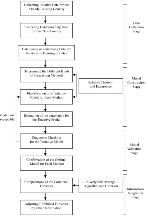
The forecasting procedure of analogy method for a new service will involve historical data already in existence in other countries, its application to the new country and comparison of characteristics between two countries. And the procedure of developing forecasts for a new service, involving the combinations of forecasts, is shown in Figure 1. This procedure can be described as following consecutive steps:

Step 1: Collect the subscriber number of this service and relative socio-economic data series for other country that already in existence.

Step 2: Collect corresponding socio-economic data series for this new country too. Step 3: Calculate their relationship or conversion ratio between the subscriber number

and socio-economic data for other country that are already in existence.

Step 4: Determine to construct independent and different kind of models to the subscriber data using socio-economic data, or time series models (such as polynomial trend model or exponential smoothing model) to the conversion ratio for other country already in existence.

Step 5: Estimate and Evaluate models. This step is often called diagnostic checking. The object is to find out how well the model fits the data. If each model is acceptable then go step 6, otherwise back step 4 to reconsider other models.

Figure 1: A New Procedure of Developing Forecasts for New Services

Collecting Relative Data for the Already Existing Country

Determining the Different Kinds of Forecasting Methods

Identification of a Tentative Model for Each Method

Estimation of the parameters for the Tentative Model

Diagnostic Checking for the Tentative Model

Confirmation of the Optimal Model for Each Method Model not

Acceptable

Computations of the Combined Forecasts

A Weighted-Average Algorithm and Criterion

Relative Theorem and Experience

Model Construction

Stage

Model Validation

Stage

Information Integration

Stage Collecting Corresponding Data

for this New Country

Calculating or conversing Data for the Already Existing Country

Data Collection

Stage

Step 7: Adjust combined forecasts to final potential demand of this new service. Since the combined forecasts are derived from technical or structured models, sometimes, we can use market research or expert opinions to adjust these combined forecasts so to more the real potential demand of this new service market nearly. Therefore, the purpose of this step is an attempt to model the decision process of judgmental forecasting revision in a structured approach.

From above descriptions of main steps, we can find there are two very important assumptions that have to be considered when we use the analogy method to forecast the potential demand of a new service:

(1) There have the most similar socio-economic development trace to convert forecasts between these two countries.

(2) The forecasting models, used in the procedure, have to follow their own statistical assumptions.

3. A METHOD OF OBTAINING THE COMBINED FORECAST

The usual approach to forecasting involves choosing a forecasting method among several candidates and using that method to derive forecasts. However, forecasts from one given method may provide some useful information which is not handled in forecasts from the other methods. Hence, it seems reasonable to consider aggregating information by generating forecasts from independent and different kind of models, and then combining these forecasts for one new service demand. In this manner, the ultimate forecasts should contain more information than is the case when only a single model is used [8].

Therefore, in this section, we consider that one combined forecast could be obtained by a linear combination of the k sets of forecasts, and these forecasts are derived from k different kind of models. We give a weight w1 to the first model set, a weight w2

to the second model set, a weight w3 to the third model set, and so on. That is, the linear

combination is

,

c T

f =w1 f1,T+w2 f2,T+ …

+(1-1

1 k

i i

w

−

=

∑

where fc T, is the combined forecast at time T, f1,T is the forecast at time T from the first

model, f2,T is the forecast at time T from the second model, and fk T, is the forecast at

time T from the last model.

There are many ways to determine these weights. The problem is how best to do it. In this paper, we wish to choose a method that could yield low forecast errors for the combined forecasts. The variance of errors in the combined forecast 2

c

σ can be written as

following:

2 c

σ =Var (fc T, )=Var (w1 f1,T+w2 f2,T+ …

+(1-1

1 k

i i

w

−

=

If the forecasts are independent among these k independent and different kind of models, then above formula could be rewritten as following:

2 c

σ =w12 2 1 σ +w22

2 2

σ + …

+(1-1 1 k i i w − =

∑

where σi2 is variance of the i-th model.

Now, for minimizing the combined variance, the above equation can be differentiated with respect to w₁,w₂,…,w_k-1 individually and equating to zero, and we can get general weight wi as followings:

i

w =

1 1 2 2 1 2

2 2 2

1

1 2

1

1 1 1 ( ... ) k k k k C j j i C j j k σ σ σ

σ σ σ

−

−

=

=

Π ×

Π + + +

=

2

2 2 2 1 2

1

1 1 1 ...

i

k

σ

σ +σ + +σ

i = 1, 2,…, k-1

k

w = 1 -

1 1 k i i w − =

∑

In the case where k=2 and k=3, we can rearrange wi as followings:

(1) When k = 2, w1 will be 2 2 2 2 1 2

σ

σ +σ and w2will be

2 1 2 2 1 2

σ

σ +σ .

(2) When k = 3, w1 will be

2 2 2 3 2 2 2 2 2 2 2 3 1 3 1 2

σ σ

σ σ +σ σ +σ σ ,

2

w will be

2 2 1 3 2 2 2 2 2 2 2 3 1 3 1 2

σ σ

σ σ +σ σ +σ σ , and w3 will be

2 2 1 2 2 2 2 2 2 2 2 3 1 3 1 2

σ σ

σ σ +σ σ +σ σ .

Usually, the true error variance σi2 under a given model will be unknown. In

practice, we can use MSEi(mean of squared forecast errors) to estimate

2 i

σ .

4. THE EMPIRICAL CASE

In order to illustrate the feasibility of this forecasting procedure for a new service, in this section, we will refer to the growth trend of PHS in Japan and use the forecasting procedure, described in the second section, to forecast the potential demand of low-tier phone in Taiwan. The practical forecasting steps are described as followings:

Step 2: We collect the population (each half a year), from 1995 to 1999, in Taiwan (shown in row 3 of 2).

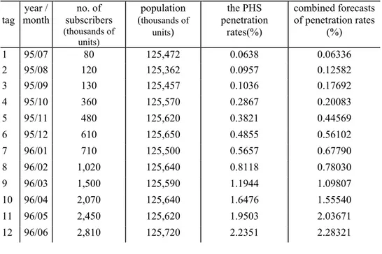
Step 3: From the data of Step 1, we can calculate the PHS penetration rates in Japan (shown in column 5 of Table 1).

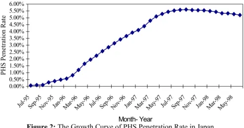
Step 4: A plot of the PHS penetration rate data in Japan versus time is given in Figure 2. From the growth curve pattern in Figure 2, we can find that the penetration rate slightly declines in the 28th period (Oct. of 1997). But it seems still reasonable to use or consider the third-order polynomial trend method, the triple exponential smoothing method, and the logistic regression method to construct different kind of models to PHS penetration rates in Japan.

Step 5: Now, we use the considered methods in Step 4 and the PHS penetration rate data in Table 1 to construct different kind of models. By model selecting process, three kind of optimal models are described as followings:

A. The First Model: The Third-Order Polynomial Trend Model

The estimation of the parameters in this optimal trend model may be obtained by using regression techniques. The estimated model and relative statistics are:

Penetration rate(%) = –0.001900 + 0.020265tag2– 0.000461tag3

(–0.033) (46.545)** (–36.845) **

MSE=0.02928 R-SQUARE=0.9937

Table 1: The No. of PHS Subscribers and Relative Data in Japan

tag year / month

no. of subscribers (thousands of

units)

population (thousands of

units)

the PHS penetration

rates(%)

combined forecasts of penetration rates

(%)

1 95/07 80 125,472 0.0638 0.06336

2 95/08 120 125,362 0.0957 0.12582

3 95/09 130 125,457 0.1036 0.17692

4 95/10 360 125,570 0.2867 0.20083

5 95/11 480 125,620 0.3821 0.44569

6 95/12 610 125,650 0.4855 0.56102

7 96/01 710 125,500 0.5657 0.67790

8 96/02 1,020 125,640 0.8118 0.78030

9 96/03 1,500 125,590 1.1944 1.09807

10 96/04 2,070 125,640 1.6476 1.55540

11 96/05 2,450 125,620 1.9503 2.03671

Table 1 (Cont.)

13 96/07 3,230 125,760 2.5684 2.51725

14 96/08 3,580 125,660 2.8490 2.84445

15 96/09 3,950 125,740 3.1414 3.11947

16 96/10 4,310 125,860 3.4244 3.41590

17 96/11 4,620 125,900 3.6696 3.70399

18 96/12 4,936 125,940 3.9193 3.94452

19 97/01 5,166 125,760 4.1078 4.19355

20 97/02 5,522 125,920 4.3853 4.36995

21 97/03 6,030 125,870 4.7907 4.65978

22 97/04 6,423 125,950 5.0996 5.08561

23 97/05 6,655 125,970 5.2830 5.34237

24 97/06 6,859 126,020 5.4428 5.42665

25 97/07 6,965 126,070 5.5247 5.51287

26 97/08 7,028 125,980 5.5787 5.54128

27 97/09 7,068 126,070 5.6064 5.56824

28 97/10 7,019 126,170 5.5631 5.58672

29 97/11 7,007 126,200 5.5523 5.53254

30 97/12 6,992 126,270 5.5373 5.53326

31 98/01 6,924 126,110 5.4904 5.52964

32 98/02 6,862 126,320 5.4322 5.47697

33 98/03 6,728 126,220 5.3304 5.40580

34 98/04 6,725 126,310 5.3242 5.28090

35 98/05 6,653 126,300 5.2676 5.27344

36 98/06 6,569 126,320 5.2003 5.18409

Table 2: The Half a Year Population Data of Taiwan

Unit: thousands

Tag 1 2 3 4 5 6 7 8 9 10

F.-J. Lin / Forecasting Telecommunication New Service Demand by Analogy Method 104 0.00% 0.50% 1.00% 1.50% 2.00% 2.50% 3.00% 3.50% 4.00% 4.50% 5.00% 5.50% 6.00% Jul-9 5 Sep -95 N ov-95 Ja n-96 M ar-96 Ma y-96_Jul-96

Se p-96 N ov-96 Ja n-97 Mar-9 7 Ma y-97_Jul-97

Se p-97 No v-97 Ja n-98 Mar-9 8 M ay-98 Month- Year PHS P enetration Rate

Figure 2: The Growth Curve of PHS Penetration Rate in Japan

B. The Second Model: The Triple Exponential Smoothing Model

When we use a value of the smoothing constant equal to α = 0.05, we find that the mean of squared forecast errors for 36 observations equals 2.64077. In a similar manner, simulated forecasting of the penetration rate data is carried out using other values of the smoothing constant α . The mean of squared forecast errors for values of

α between 0.05 and 0.99 in increments of 0.05 are given in Table 3. We find that α = 0.65 is the optimal value of the smoothing constant when we use these penetration rates to build a triple exponential smoothing model.

Table 3: The MSE for Different Values of α

α MSE α MSE α MSE α MSE

0.05 2.64077 0.10 0.63609 0.15 0.16691 0.20 0.05792 0.25 0.02844 0.30 0.01823 0.35 0.01367 0.40 0.01125 0.45 0.00982 0.50 0.00896 0.55 0.00845 0.60 0.00817

0.65 0.00808 _{0.70 0.00813 0.75 0.00833 0.80 0.00866}

0.85 0.00917 0.90 0.00989 0.95 0.01088 0.99 0.01193 Note: αis smoothing constant

Therefore, we can obtain updated values of the smoothed statistics ST,

[2] T S and

[3] T

S by using following smoothing equations during building this triple exponential smoothing model:

T

S = 0.65yT+0.35ST-1

[2] T

S = 0.65ST+0.35

[2] -1 T S [3] T

S = 0.65ST[2]+0.35 [3]

-1 T S

where yT is the penetration rate at time T, and ST-1,

[2] -1 T

S , ST[3]-1 are values of the

C. The Third Model: The Logistic Regression Model

The logistic regression curve is different from the linear and exponential curves by having saturation or ceiling level. Therefore, we use non-linear least squares iterative process to estimate its parameters. The estimated model and relative statistics are

Penetration rate(%) = 5.53254

1 exp(43.12777 0.27008 tag)+ − ×

MSE=0.03309 R-SQUARE=0.9981

Step 6: In this step, following the method of obtaining combined forecast described in the third section, we use weighted average to combine three models’ forecasts by their estimated variances MSE. That is, the combined forecast would be obtained by a linear combination of three sets of forecasts in this case, giving a weight w1

to the first model set, a weight w2 to the second model set, and a weight w3=1– 1

w–w2 to the third model set. The linear combination is ,

c T

f =w1 f1,T+w2 f2,T+(1–w1–w2) f3,T

where fc T, is the combined forecast at time T, f1,T is the forecast at time T from

the first model, f2,T is the forecast at time T from the second model, and f3,T is

the forecast at time T from the third model.

Now, if the forecasts are independent among these three models, then for minimizing the combined variance, as described in the third section, the above equation can be differentiated with respect to w1 and w2 individually and

equating to zero, so that we can get weight w1, w2 and w3 as followings:

1

w

=

2 3 1 3 1 2

MSE MSE

MSE MSE +MSE MSE +MSE MSE

2

w

=

2 3 1 3 1 2

MSE MSE

MSE MSE +MSE MSE +MSE MSE

3

w

=

2 3 1 3 1 2

MSE MSE

MSE MSE +MSE MSE +MSE MSE

where MSEi is the estimated error variance of the i-th model.

From the formula, the weights of these three models can be obtained as followings:

1

w=0.1815, w2=0.6578, w3=0.1607

then, the combined forecast at time T can be obtained from following:

,

c T

f =0.1815f1,T+0.6578f2,T+0.1607f3,T

Although low-tier phone service operators have been granted the concessions and licenses in 1999 in Taiwan, the formal operation and service was waited to for till latter half of 2001. And as described before, we suppose that the Taiwanese socio-economic environment and telecommunication industry development are similar as Japanese. Hence, in our study, it is reasonable that we suppose the low-tier phone penetration rate in Taiwan in January 2001 to be equal to the PHS penetration rate in Japan in July 1995. To carry on, we first use the half a year population data of Taiwan (shown in Table 2) to build the following first-order trend model to predict the population from December 2000 to June 2002 (shown in column 3 of Table 4):

Population = 21115 + 93.060606×tag tag=1,2,…

(3052.822) (83.484)**

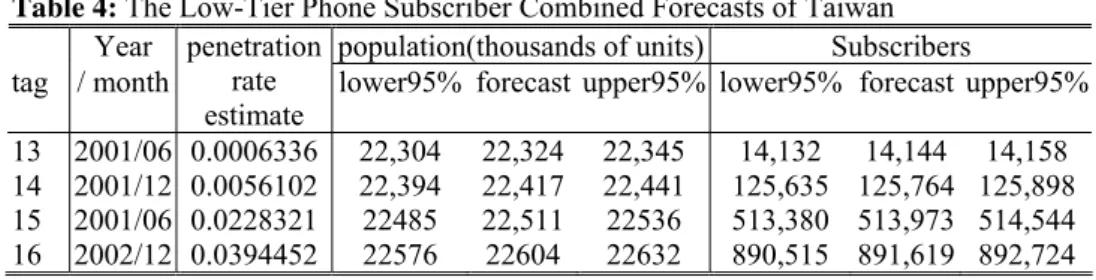
And then, we transfer the estimated penetration rates to low-tier phone subscriber combined forecasts of Taiwan in column 4 of Table 4.

Table 4: The Low-Tier Phone Subscriber Combined Forecasts of Taiwan

Year population(thousands of units) Subscribers tag / month

penetration rate estimate

lower95% forecast upper95% lower95% forecast upper95%

13 2001/06 0.0006336 22,304 22,324 22,345 14,132 14,144 14,158 14 2001/12 0.0056102 22,394 22,417 22,441 125,635 125,764 125,898 15 2001/06 0.0228321 22485 22,511 22536 513,380 513,973 514,544 16 2002/12 0.0394452 22576 22604 22632 890,515 891,619 892,724

From Table 4, in the first half year of beginning operation, we can estimate that potential demand will be 125 thousands at most by our technical procedure. It is very close to actual 120 thousands subscribers that the operator announced. And the first year of beginning operation will be about 513 thousands.

5. CONCLUSIONS

In this paper, we integrate the concept of analogy method and the idea of combined forecast to establish the procedure of forecasting telecommunication new service demands. In this context, we first describe all the steps of the forecasting procedure, and then, we provide a way to determine the weights of obtaining one combined forecast that could yield lower mean of squared forecast error. Finally, for illustrating the feasibility of this forecasting procedure for a new service, we forecast the potential demand of low-tier phone in Taiwan using this technical forecasting procedure. The idea of combined forecast and analogy method are not new. However, in this paper we integrate them in a new way and illustrate that it is feasible for developing new service forecasts.

REFERENCES

[1] Bowerman, B.L., and O’Connell, R.T., Forecasting and Time Series: An Applied Approach, 3rd ed, Wadsworth, Inc., Belmont, California, 1993.

[2] CCITT: Forecasting New Telecommunication Services, CCITT Recommendation E.508, 1-18 1992.

[3] Chang, H.J., and Lin, F.J., "Forecasting telecommunication traffic using the enhanced stepwise projection multiple regression method", Yugoslav Journal of Operation Research, 5 (1995) 271-288.

[4] Chang, H.J., and Lin, F.J., "Forecasting with the enhanced stepwise data adjustment regression method", The Asia-Pacific Journal of Operational Research, 15 (1998) 225-238.

[5] Dartois, J.P., and Gruszecki, M., "Demand forecasting for new telecommunication services", Traffic Engineering for ISDN Design and Planning, 161-172 (1988).

[6] Draper, N., and Smith, H., Applied Regression Analysis, 2nd ed., John Wiley & Sons, Inc., New York, 1981.

[7] Kimura, G. et al., "Service demand forecasting and advanced access network architectures", ITC, 14 (1994) 1301-1310.

[8] Makridakis, S., and Winkler, R.L., "Averages of forecasts: Some empirical results", Management Science, 29(9) (1983) 987-996.

[9] Stordahl, K., and Murphy, E., "Forecasting long-term demand for services in the residential market", IEEE Communications Magazine, 33(2) (1995) 10-49.