Braz. J. Chem. Eng. vol.30 número4

ISSN 0104-6632 Printed in Brazil

www.abeq.org.br/bjche

Vol. 30, No. 04, pp. 909 - 921, October - December, 2013

Brazilian Journal

of Chemical

Engineering

THE USE OF GAUSS-HERMITE QUADRATURE IN

THE DETERMINATION OF THE MOLECULAR

WEIGHT DISTRIBUTION OF LINEAR POLYMERS

BY RHEOMETRY

T. M. Farias

1

, N. S. M. Cardozo

1

and A. R. Secchi

2*

1

GIMSCOP/LATEP - Chemical Engineering Department, Federal University of Rio Grande do Sul, Escola de Engenharia, Departamento de Engenharia Química, Universidade Federal do Rio Grande do Sul

(UFRGS), Phone: + (55) (51) 3316-3528, Fax: + (55) (51) 3316-3277, R. Eng. Luiz Englert, s/n, CEP: 90040-040, Porto Alegre - RS, Brazil.

E-mail: [email protected]; [email protected] 2

COPPE/PEQ - Federal University of Rio de Janeiro, CT, Rio de Janeiro - RJ, Brazil.

Universidade Federal do Rio de Janeiro (UFRJ), Instituto Alberto Luiz Coimbra de Pós Graduação e Pesquisa de Engenharia, Phone: + (55) (21) 2562-8301, Fax: + (55) (21) 2562-8300, Av. Horácio Macedo 2030, Centro de Tecnologia, Bloco G, Cidade Universitária, Fundão, CEP: 21941-914, Rio de Janeiro - RJ, Brazil.

E-mail:[email protected]

(Submitted: May 6, 2012 ; Revised: December 11, 2012 ; Accepted: December 16, 2012)

Abstract - The molecular weight distribution (MWD) and its parameters are of the fundamental importance in the characterization of polymers. Therefore, the development of techniques for faster MWD determination is a relevant issue. This paper aims at implementing one of the relaxation models from double reptation theory proposed in the literature and analyzing the numeric strategy for the evaluation of the integrals appearing in the relaxation model. The inverse problem, i.e., the determination of the MWD from rheological data using a specified relaxation model and an imposed distribution function was approximated. Concerning the numerical strategy for the evaluation of the integrals appearing in the relaxation models, the use of Gauss-Hermite quadrature using a new change of variables was proposed. In the test of samples of polyethylene with polydispersities less than 10, the application of this methodology led to MWD curves which provided a good fit of the experimental SEC data.

Keywords: Rheology; Inverse Problem; Gauss-Hermite Quadrature.

INTRODUCTION

The characterization of a polymer in terms of molecular weight distribution (MWD) requires not only the determination of a single average value but also additional moments of this distribution. This characterization is of fundamental practical importance because the MWD has a direct influence on the processability and final properties of a polymeric material, being one of the key variables in the control of polymerization processes.

Although the MWD is usually determined by gel permeation chromatography (GPC), some limitations of this technique, such as cost and time consumption, have led to the study of alternative methods for its determination. In this context, methods based on the use of relaxation models, which describe the linear viscoelastic properties of polymers as a function of the MWD, have received great attention in the literature.

technique, the conversion of dynamic elastic modulus data (G´(ω)) into distribution curves of molecular weight was done by a simple analytical expression, obtained from considerations regarding the relation between the relaxation mechanisms of polymer melts and the MWD. However, the distribution curves obtained by this method were characterized by presenting artificial multimodality, i.e., multimodality not found in the analysis by GPC. Applying a similar methodology for data of relaxation modulus G(t), Tuminello and Mc Grory (1990) also reported artifi-cial bimodality for some samples.

Recently, methods based on reptation and double reptation theories have been presented (Wasserman, 1995; Léonardi, 1999; Léonardi et al., 2002; van Ruymbeke et al., 2002a; Peirotti and Deiber, 2003; Guzmán et al., 2005; Nobile and Cocchini. 2008; Friedrich et al.. 2009). To obtain the MWD by these methods, it is necessary to calculate the relaxation spectrum from G´(ω) and G´´(ω) experimental data, impose a distribution function to represent the MWD, select a molecular model that incorporates the concept of double reptation to represent the relaxation process of the polymer molecules, and approximate an inverse problem to obtain the parameters of the distribution function selected to represent the MWD from experimental data of dynamic moduli.

The use of an arbitrary distribution function is based on the idea that the MWD is the result of random events that occur during the polymerization reaction and is controlled by the characteristics and conditions of the polymerization process. Conse-quently, it is expected that common characteristics are found between the MWD of different polymers. Several mathematical functions have been used in the literature to describe the molecular weight distribution of polymers (Rogosic et al., 1996; Fried, 2003) including the Flory-Schulz, the Gaussian dis-tribution and the Generalized Exponential (GEX) function (Gloor, 1983), with GEX standing out in terms of goodness of fit to experimental data of MWD derived from techniques like GPC.

Regarding the approximation of the inverse problem involved, two different approaches are usually used in these methods: i) explicit calculation of the relaxa-tion spectrum, and ii) use of the parametric method proposed by Schwarzl (1971) in order to avoid the explicit calculation of the relaxation spectrum. For the explicit calculation of the relaxation spectrum, the application of Tikhonov regularization is sug-gested in the literature (Honerkamp and Weese, 1989; Weese, 1992). In the parametric approach, the dynamic moduli G´ and G´´ are obtained through the inversion of G(t) by using the Schwarzl relations

(van Ruymbeke et al., 2002a), derived from approxi-mations by Fourier transforms.

Besides the intrinsic ill-posedness in the approxi-mation of the inverse problem of retrieving the parameters of the molecular weight distribution from the molecular models for the moduli (van Ruymbeke

et al., 2002b; Léonardi et al., 1998; Léonardi, 1999; Léonardi et al., 2002; van Ruymbeke et al., 2002a; Peirotti and Deiber, 2003; Cocchini and Nobile, 2003; Llorens et al., 2003), another key point in these methods is the efficiency of the numerical scheme used to evaluate the integrals which appear in the mixing rules used to apply the molecular models to polydisperse samples. These integrals relate the shear relaxation modulus of the entangled polymer with the MWD and have to be calculated recursively in the approximation of the inverse problem, which is basically an optimization problem. However, there is little information in the literature concerning specifi-cally the influence of the integration method on the performance of the methods for rheological data-based determination of MWD.

Due to the intrinsic characteristics of the problem under consideration, the use of integration methods based on orthogonal polynomials appears as an interesting alternative. Orthogonal polynomials are widely used in the approximation of inverse problems in the areas of physics and mathematics. In polymer engineering, they are used in the prediction of the evolution of the MWD during polymerization reactions through the solution of chemical kinetics models, representing the MWD as a series of Laguerre (Saidel and Katz, 1968)or Lagrange (Seferlis and Kiparissides, 2002) polynomials, whose weight function is the

Flory-Schulz distribution (Coni Jr., 1992). Peirotti and Deiber (2003) developed a procedure to estimate the density distribution function (DDF) fw(M) from the double reptation mixing rule for binary and polydisperse blends using data of relaxation moduli. Their approach uses the normal and gamma func-tions to represent the DDF, expanding these distribu-tion funcdistribu-tions in Hermite and Laguerre polynomials, respectively, to evaluate the double reptation mixing rule. However, further research is required to find both a robust algorithm and a complete relaxation law to consider multimodal and highly polyidisperse samples.

transfor-mation was proposed for the GEX distribution function in order to allow the use of Gauss-Hermite quadrature to evaluate the integrals appearing in the mixing rules required for the determination of the MWD and the results obtained with the proposed strategy are compared to those obtained with the classical trapezoidal integration method. The MWDs obtained by applying the proposed methodology were compared with size-exclusion chromatography data of commercial samples of polyethylene with polydispersities less than 10. This polydispersity index limit was defined according to preliminary tests which indicated that the methodology based on the

des Cloizeaux model is not appropriate for high polydispersity indexes. Additionally, within this range of polydispersity, theoretical and experimental data are available in the literature for comparison purposes.

METHODOLOGY

Inverse Problem for the Determination of the MWD

The inverse problem for the determination of the MWD was written using well-established strategies described in the literature. Firstly, to apply the theory of double reptation to polydisperse polymers, it is necessary to specify a mixing rule for prediction of rheological properties of the polydisperse polymer sample from the contribution of the individual molecules. The following double reptation mixing rule (van Ruymbeke et al., 2002b; Tsenoglou, 1991; Léonardi et al., 2000; Vega et al., 2012) was used:

1 0

( ) _N ( , ) ( )

LL

G t G F t M P M dM

β +∞

β

⎡ ⎤

⎢ ⎥

= _{⎢ ⎥}

⎣

∫

⎦

(1)

where G_N0 is the plateau modulus, LL is the lower limit of molecular weight for the integration, F(t,M) is a kernel function describing the relaxation behaviour of a monodisperse polymer of molecular weight M,

P(M) is the distribution function used to represent the MWD of the sample, and P(M) dM is the nor-malized probability of finding a chain with molecu-lar weight between M and M + dM.

In the original model of the double reptation (des Cloizeaux, 1988) the value of the exponent β in Equation 1 is 2, but different values have been suggested in the literature (van Ruymbeke et al.,

2002b; Maier et al., 1998). In this work, as suggested by van Ruymbeke et al. (2002b), β= 2.25 was used.

Regarding the lower limit of the integral (LL), the use of either Me (van Ruymbeke et al., 2002b) or 2Me

(Léonardi et al., 1998; Léonardi, 1999; Léonardi et al., 1998; Léonardi et al., 2000; Léonardi et al., 2002) has been suggested in the literature. The molecular model of des Cloizeaux (1990)was used to represent the relaxation process of the polymer molecules. This model, which considers the diffusion mechanism of stress points along the chain, is able to better describe the mechanisms of reptation combined with the fluctuations of the tube length. It is given by:

(

)

1

2

2 2

8 1

( , ) exp ( , )

i ODD

F t M i U t M i

β _{= −}

π

∑

(2)

where iODD means the sum over odd numbers of i,

and U(t,M) is evaluated as:

* *

( , )

( ) ( )

rept rept

t M M t U t M g

M M M M

⎛ ⎞

=_λ + ⎜_⎜ ⎟_⎟ λ

⎝ ⎠ (3)

where g can be approximated as in the following equation, according to van Ruymbeke et al. (2002b):

0.5 0.5 0.5

( ) [ ( ) ]

g q = − +q q q+ πq + π (4) and λrept is given by λrept = KM3. The parameter M* is

related to the molecular weight between entangle-ments (Me) and the parameter K, which can be

deter-mined from experimental measures of viscosity as a function of the molecular weight, depends on the nature of the material and on the temperature. More details on the des Cloizeaux model can be found in the literature (des Cloizeaux, 1990; Maier et al., 1998; van Ruymbeke et al., 2002b).

The GEX function was used as the imposed MWD distribution, in the functional form proposed by Léonardi et al. (2002):

( )

1

exp

k

ref ref

m

ref

m M P M

k M M

m

M M

⎛ ⎞ = _{⎛ +} ⎜_⎜ ⎟_⎟ ⎞ ⎝ ⎠ Γ⎜_⎝ ⎟_⎠

⎡ _{⎛ ⎞} ⎤ ⎢_{−⎜⎜ ⎟⎟} ⎥ ⎢ _{⎝ ⎠} ⎥

⎣ ⎦

(5)

where m, k and Mref are the parameters which define

on these parameters, the expressions for the three first moments of a MWD described by the GEX func-tion can be expressed as (Léonardi et al., 2002; van Ruymbeke et al., 2002a; Cocchini and Nobile; 2003):

1 n ref k m M M k m + ⎛ ⎞ Γ⎜_⎝ ⎟_⎠ =

⎛ ⎞ Γ⎜ ⎟_{⎝ ⎠}

(6) 2 1 w ref k m M M k m + ⎛ ⎞ Γ⎜_⎝ ⎟_⎠

= ₊

⎛ ⎞ Γ⎜_⎝ ⎟_⎠

(7) 3 2 z _ref k m M M k m + ⎛ ⎞ Γ⎜_⎝ ⎟_⎠

= ₊

⎛ ⎞ Γ⎜_⎝ ⎟_⎠

(8)

and the polydispersity index is given by:

2 2 1 w n k k M m m PD

M _k m

+

⎛ ⎞ ⎛ ⎞ Γ_{⎜ ⎟ ⎜ ⎟}Γ ⎝ ⎠ ⎝ ⎠ = =

+ ⎛ ⎞ Γ⎜_⎝ ⎟_⎠

(9)

Formulation of the Parameter Estimation Problem

The optimal GEX parameters were determined by a χ2 minimization procedure, using the following objective function:

(

)

2 ´ ´ ´ 2 2 ´´ ´´ , , , 1 ´´ 1 min 2 ₌ ⎫ ⎧ ⎡ _{⎛ − ⎞} ⎤ ⎪ ⎪ ⎢ _{⎜ ⎟ ⎪}⎥ ⎪ ⎢ ⎜ ⎟ ⎥ ⎪ _{⎢ ⎝ ⎠ ⎥}⎪

χ = _{⎨ ⎬}

⎢ ⎛ − ⎞ ⎥ ⎪ _{⎢ ⎜+ ⎟ ⎥}⎪ ⎪ _{⎢ ⎜ ⎟ ⎥}⎪ ⎪ ⎣ ⎝ ⎠ ⎦⎪ ⎩ ⎭

∑

i i E i ref i i i E M N E

k m M M _{E i}

E M

E

G G G N _{G G}

G

(10)

where ´

i

E

G and ´´

i

E

G are the experimental data measured at the frequencies ωi for i = 1, 2, 3 .... NE, NE is the

number of points in the frequency set, and ´

i

M

G and

´´

i

M

G are the theoretical values of the moduli at each frequency ωi. As suggested by van Ruymbeke et al.

(2002a), G´M_i and G´´M_i were calculated from the

relaxation modulus G(t) using the Schwarzl relations (Schwarzl, 1971):

( ) ( )

( ) ( )

( ) ( )

( ) ( )

( ) ( )

( ) ( )

( ) ( )

(

) ( )

(

) (

)

´ 1 2 3 4 5 6 7 8

~ 4 8

2 4

2 / 2

/ 4 / 2 / 8 / 4 / 16 / 8 / 64 / 32 ...

ω + ⎡_⎣ − ⎤_⎦ + ⎡_⎣ − ⎤_⎦ + ⎡_⎣ − ⎤_⎦ + ⎡_⎣ − ⎤_⎦ + ⎡_⎣ − ⎤_⎦ + ⎡_⎣ − ⎤_⎦ + ⎡_⎣ − ⎤_⎦ + ⎡_⎣ − ⎤_⎦+ M

G G t a G t G t a G t G t a G t G t a G t G t a G t G t a G t G t a G t G t a G t G t

(11)

( )

( ) ( )

( ) ( )

( ) ( )

( ) ( )

( ) ( )

(

) ( )

(

) (

)

(

) (

)

´´ 1 2 3 4 5 6 7 8

~ 2 4

2 / 2

/ 4 / 2 / 8 / 4 / 16 / 8 / 64 / 32

/ 256 / 128 ...

ω − ⎡_⎣ − ⎤_⎦ + ⎡_⎣ − ⎤_⎦ + ⎡_⎣ − ⎤_⎦ + ⎡_⎣ − ⎤_⎦ + ⎡_⎣ − ⎤_⎦ + ⎡_⎣ − ⎤_⎦ + ⎡_⎣ − ⎤_⎦ + ⎡_⎣ − ⎤_⎦+ M

G b G t G t b G t G t b G t G t b G t G t b G t G t b G t G t b G t G t b G t G t

(12)

where ai´s and bi’s are the coefficients that define the

parametric method and can be checked in the work of Schwarzl (1971). The value of t used in the calculation is equal to the inverse of the frequency at a given point. The values of G(t) were obtained using Equations (1)-(5), with the integrals appearing in Eq. (1) being evaluated either by the conventional trapezoidal rule or by the Gauss-Hermite quadrature proposed in the next section.

Due to the large range of possible values for the GEX parameters k, m, and Mref, and the observed

correlation among these parameters, the optimization problem described by Eq. (10) was solved considering an auxiliary parameter ζ:

1

m ref

M

ζ= (13)

1 m ref

M = ζ− (14)

Approximation of the Integral Relating the Shear Relaxation Modulus by Gauss-Hermite Quadrature

Based on the orthogonality of Hermite polyno-mials with respect to the weight function ω(x) = exp(−x2) in the interval (−∞, +∞), Gauss quadrature can be used to approximate the following integral:

1

( ) ( ) ( )

quad

N

i i i

x f x dx w f x

+∞

= −∞

ω ≈

∑

∫

(15)

where the abscissas xi are the roots of the Hermite

polynomial of degree Nquad, and wi are the weights of

the quadrature. This integral is exact when f(x) is a polynomialof degree less than 2 Nquad (Abramowitz

and Stegun, 1972; Press et al., 1988). To apply the Gauss-Hermite quadrature in approximating the inverse problem, the first step is to rewrite the GEX function (Equation 5) in terms of a weight function

ω(x) = exp(−x2) to later apply the double reptation mixing rule (Equation 1). By defining the following terms:

1/2

2

n w

ref

k

M M m

k M

m

+ ⎡_Γ⎜⎛ ⎞⎤

⎟ ⎢ _{⎝ ⎠}⎥

⎢ ⎥

Δ = =

⎛ ⎞ ⎢ _{Γ⎜ ⎟} ⎥ ⎢ _{⎝ ⎠} ⎥

⎣ ⎦

(16)

ln( )

c PD

φ = (17)

and

ln

ref

M M x

⎛ ⎞

⎜ ⎟

⎜ _Δ⎟

⎝ ⎠

= _φ (18)

where c in Eq. (17) is a scaling constant used to regulate the distribution of the quadrature points in the range of molecular weights of interest, the GEX function can be expressed by the following equation:

(

)

( )

1

exp exp

= _{⎛ + ⎞}Δ Γ⎜_⎝ ⎟_⎠

⎡ φ −Δ φ ⎤

⎣ ⎦

k

ref

m

m P x

k M

m

k x m x

(19)

Equation (19) can be written in terms of the weight function ω(x) as follows:

2

( ) ( ) exp( )

P x =g x −x (20)

where:

(

)

2

( )

1

exp exp

= _{⎛ + ⎞}Δ Γ⎜_⎝ ⎟_⎠

⎡ φ −Δ φ + ⎤

⎣ ⎦

k

ref

m

m g x

k M

m

k x m x x

(21)

Then the Gauss-Hermite quadrature can be applied to calculate the relaxation module G(t) repre-sented by the double reptation mixing rule. First,

P(M) dM is written as P(x) dx:

( )

( ) _ref exp ( )

P M dM =M Δ φ φx P x dx (22)

Thus, applying this change of variable to the double reptation mixing rule, Eq. (1), results in:

0 * 2

( ) _N ( ) exp ( )

G t G g x x dx

β +∞

−∞

⎡ ⎤

⎢ ⎥

= −

⎢ ⎥

⎣

∫

⎦

(23)

where:

( )

1

*

( ) ( ) ( , ) _ref exp

g x =g x Fβ t x M Δ φ φx (24) The double reptation mixing rule can then be calculated in terms of Gauss-Hermite quadrature by the following equation:

0 *

1

( ) ( )

quad

N

N i i

i

G t G w g x

β

=

⎡ ⎤

⎢ ⎥

≈

⎢ ⎥

⎣

∑

⎦

       (25)

Direct Problem

Before treating the inverse problem described previously, a direct problem was analyzed in order to verify the implementation of molecular models used in this work. This direct problem consisted of calcu-lating the linear viscoelastic properties of a reference sample by using the molecular weight distribution, obtained from its specific GEX function, in the double reptation mixing rule. A polystyrene sample charac-terized by van Ruymbeke et al. (2002a) was used as reference in this analysis, since for this sample both the rheometric data and the GEX function parameters were available.

Materials and Rheological Measurements

Two commercial grades of high density poly-ethylene (HDPE) were used. These samples, named PE1 (homopolymer used for injection) and PE2 (copolymer used for injection), were kindly provided by the Technology and Innovation Centre of BRASKEM

S.A., as well as their GPC curves The referred GPC analyses were performed in a Waters model GPC/ V2000 liquid chromatograph with RI detection, viscosimetric detector (DV), four columns (Toso-Hass HT3, HT4, HT5, and HT6) and a pre-column (500Å), using narrow PS standards for calibration purposes and a standard polydisperse polyethylene to check the calibration curve. The size-exclusion chromatography (SEC) was carried out at 140 °C in 1,2,4-trichlorobenzene enhanced with BHT. Since both PE1 and PE2 are produced by a catalytic process which does not generate long chain branches (LCBs), the GPC/SEC results for these two materials are expected to be free of any systematic error due to the presence of LCBs. The values of number and weight average molecular weight and polydispersity index of these polyethylenes are presented in Table 1. Table 1: Available information of the samples studied.

Sample Available information M n

(g/mol)

w M

(g/mol)

/ w n

M M

PE1

HDPE, homopolymer, injection

21000 70000 3.3

PE2 HDPE, copolymer,

injection 14000 80000 5.7

Since the parameters β (Equation (1)), K (Equation (3)), plateau modulus (G0_N) and molecular weight be-tween entanglements (Me) are not dependent on the

molecular weight distribution, a single value of each of these parameters was used for both samples of HDPE. These values were obtained from the literature (van Ruymbeke et al., 2002a; van Ruymbeke et al.,

2002b; Léonardi et al., 2000) and are shown in Table 2. Table 2: Constants of the des Cloizeaux model (Equations (1)-(3)) for HDPE at 190 °C.

Parameter Value Parameter Value β 2.25 M * _{[g/mol] 7.0x10}4

α 3 Me [g/mol] 1500

K [s(mol/g)α] 1.4x10-17 G0N [Pa] 2.6x10

6

Dynamic storage and loss moduli were determined using a strain-controlled rheometer (Rheoplus from Anton Paar) in the dynamic mode with a parallel plate geometry (25 mm diameter) at 190 °C. Linearity of the viscoelastic regime was checked by strain sweep tests. In order to obtain linear viscoelasticity measure-ments, strains of 5.5% for PE1 and 4.5% for PE2 were used for all the subsequent tests. The angular frequency sweep interval was 0.1-500 rads-1.

RESULTS

Check of the Implemented Routines with the Direct Problem

The three sets of parameters k, m, and Mref

presented by van Ruymbeke et al. (2002a) for their polystyrene sample PS1 were applied in the imple-mented routines to calculate the dynamic moduli of this sample using the des Cloizeaux model. Although the three set of parameters provided quite similar results, as reported by van Ruymbeke et al. (2002a), all curves of moduli obtained with the implemented routines presented a systematic error characterized by a negative displacement in relation to the experimental data. This systematic error can be observed in the dashed lines of Figure 1, calculated with the parameter set k = 11.245, m = 3.922, and

Mref = 272.960. It is important to mention that these

systematic deviations are not observed in the work of van Ruymbeke et al. (2002a).

The discrepancy observed in Figure 1, i.e., the vertical shift of about 5/4 for the predicted dynamic moduli (G´and G´´) compared to the experimental data, can be related to an uncertainty in the plateau modulus (GN0 ), which is very difficult to measure

representation of the experimental data is observed (solid lines of Figure 1). This correction in the plateau modulus was used in all the remaining calculations.

102 103 104 105 106

10-3 10-2 10-1 100 101 102 103 104

G

’

,

G

’

’

(P

a)

ω (rad/s)

G’ experimental G’’ experimental G’ des Cloizeaux

G’’ des Cloizeaux

G’ des C. with correction G’’ des C. with correction

Figure 1: Experimental values of G’ and G’’ and values predicted by the direct problem using the GEX function with parameters k, m and Mref.

Performance of the Gauss-Hermite Quadrature in the Approximation of the Inverse Problem

The inverse problem was approximated for the samples PE1 and PE2 using the trapezoidal rule and Gauss-Hermite quadrature. In the case of the trape-zoidal rule, Me was adopted as the lower limit of

integration and a molecular weight of 107 g/mol was used as the upper limit of integration and the integra-tion points were equally spaced on a logarithm scale. In order to make a comparison between these integration procedures, the number of points, N, used to represent the molecular weight distribution was varied in the interval ranging from 12 to 55 points.

The parameters k, m and ζ were estimated using the Nelder-Mead algorithm as implemented in the function fminsearch of MATLAB 5.3 (The MathWorks, Inc.) with multiple starting points to skip possible local minima, followed by the Levenberg-Marquardt algorithm implemented in the function lsqnonlin of MATLAB 5.3 to refine the solution. The iterations converged when the absolute change in two succes-sive χ2 values was less than 10-6. A comparison between the estimated MWD and the results of characterization by GPC was carried out, and the dynamic moduli G´ and G´´ were predicted through the double reptation mixing rule and Schwarzl

relations (Schwarzl, 1971) and compared with experimental data. For this purpose, the optimization results were expressed in terms of the following parameters: (i) relative difference between estimated

and experimental (GPC) values of the average molecular weights M_n and M_w ( %EM_n and

%EM_w, respectively), (ii) root mean square error (RMSE) and (iii) the estimated relative integration error (EI_{method i,} ). These parameters were defined as follows:

, ,

,

% _n n calculated n GPC 100

n GPC

M M

EM

M

−

= × (26)

, ,

,

% _w w calculated w GPC 100

w GPC

M M

EM

M

−

= × (27)

2 2

´ ´ ´´ ´´

´ ´´

1

1

% %

100 100

=

⎡_{⎛ − ⎞ ⎛ − ⎞} ⎤ ⎢_{⎜ ⎟ ⎜+ ⎟} ⎥ ⎢⎜_⎝ ⎟ ⎜_{⎠ ⎝} ⎟_⎠ ⎥

⎢ ⎥

⎣ ⎦

=

+ +

∑

E

i i i i

i i

N

E M E M

E i E E

n w

G G G G

N G G

RMSE

E M E M

(28)

, 55 ,

,

,55 G H method i method i

G H

I I EI

I

− − −

= (29)

where ´

i

E

G and ´

i

M

G are the experimental and predicted values of G´, G´´_Eiand G´´_Miare the experimental and predicted values of G´´, I_{G H− , 55} is the value of the integral that represents the area under the MWD curve obtained with the Gauss-Hermite methodology using 55 quadrature points, and I_{method i,} is the value of this integral obtained with the specified method (G-H: Gauss Hermite quadrature, or TRAPZ: trapezoidal rule) and i points of quadrature. I_{G H− , 55}

was taken as representative of the exact value of the integral. Eq. (28) is similar to that presented by Borg and Pääkkönen (2009), differing in the fact that the number of experiments (NE) is inside the square root

to take the average of the square errors.

The problem was assessed using the criteria described above and, after preliminary tests, the appropriate number of points of molecular weight necessary to represent the MWD of each sample was chosen.

using the Nelder-Mead algorithm and values of the Gauss-Hermite quadrature scale constant c (Eq. 15) of 1/2 for PE1 and 1/3 for PE2, according to the following procedure: (i) testing different initial estimates for N = 8, it was found that the sets k = 5,

m = 0.15, ζ= 8 for PE1 and k = 0.5, m = 0.5, ζ= 0.1 for PE2 provide the best fit of the GPC data; (ii) the solution for the subsequent values of N tested (up to 55) was found using the optimal set of parameters found in the previous step as initial estimates.

Figure 2 shows the variation of %EM_n with the number of points of molecular weights for PE1 and PE2 considering the trapezoidal rule and Gauss-Hermite quadrature. It is possible to observe that, for both samples, a limiting value of %EM_n is obtained with the Gauss-Hermite quadrature for a high number of quadrature points, indicating convergence of the integration method. This limiting value of %EM_n

was close to 0% and was reached with N = 12 for sample PE1, while for PE2 it was around 4% and was reached with N = 16. On the other hand, the data of Figure 2 show that the trapezoidal rule provided

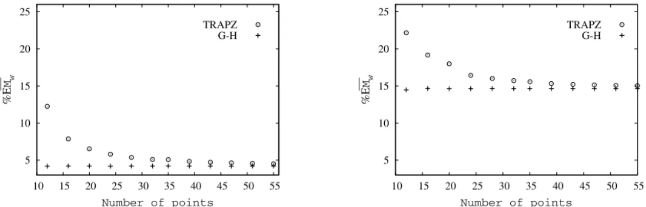
slower convergence, in such a way that a number of quadrature points higher than the maximum used here (55) would be required to achieve the limiting values of %EM_n obtained with the Gauss-Hermite quadrature. Figures 3 and 4 show that the behaviours of the Gauss-Hermite quadrature and the trapezoidal rule in terms of the resulting values of %EM_w and

RMSE are basically the same as described for %EM_n, except that the limiting values obtained by the Gauss-Hermite for %EM_w (4% for PE1 and 15% for PE2) were higher than those corresponding to %EM_n. However, in both cases the values found in the present work are of the same order of magnitude as those obtained by Léonardi et al (2002) (EM_n%=2.46and EM_w% =6.45) in studying the inverse problem for another HDPE of polydispersity index 4.6. Furthermore, Léonardi (1999) obtained

% 14.36 n

EM = and EM_w%=19.59for a HDPE sam-ple of polydispersity index 6.42, applying the GEX function and the DRMD (Double Reptation with Molecular Dynamics) model.

0 5 10 15 20 25 30 35 40

10 15 20 25 30 35 40 45 50 55

%E

M

⎯ n

Number of points

TRAPZ G-H

0 5 10 15 20 25 30 35 40

10 15 20 25 30 35 40 45 50 55

%E

M

⎯ n

Number of points

TRAPZ G-H

Figure 2: %EM versus_n number of points of molecular weight for PE1 (on the left) and PE2 (on the right) samples using the trapezoidal rule and Gauss-Hermite quadrature.

5 10 15 20 25

10 15 20 25 30 35 40 45 50 55

%E

M

⎯ w

Number of points

TRAPZ G-H

5 10 15 20 25

10 15 20 25 30 35 40 45 50 55

%E

M

⎯ w

Number of points

TRAPZ G-H

0.2 0.25 0.3 0.35 0.4 0.45 0.5

10 15 20 25 30 35 40 45 50 55

R

M

S

E

Number of points

TRAPZ G-H

0.2 0.25 0.3 0.35 0.4 0.45 0.5

10 15 20 25 30 35 40 45 50 55

R

M

S

E

Number of points

TRAPZ G-H

Figure 4: RMSEversus number of points of molecular weight for PE1 (on the left) and PE2 (on the right) samples using the trapezoidal rule and Gauss-Hermite quadrature.

The slower convergence of the trapezoidal rule with relation to the Gauss-Hermite in terms of the parameters %EM_n, %EM_w and RMSE can be ex-plained directly based on the intrinsic variation presented by each method regarding the gain in precision resulting from an increase in the number of points of integration. As can be seen in Figure 5, the values of EI_{G H i− ,} decrease rapidly to values close to zero as the number of points of molecular weight increase, while for EI_{TRAPZ i,} the decrease with the number points is much lower, mainly after around 20 points, limiting the accuracy which can be obtained.

Based on the previous discussion of the results presented in Figures 2-5, the results of the trapezoidal rule with N = 55, for both PE1 and PE2, and of the Gauss-Hermite quadrature with N =12 for PE1 and N =16 for PE2 were taken as reference in the subsequent analysis, where experimental and predicted data of MWD and moduli are compared. The values of N =12 for PE1 and N =16 for PE2

correspond to the minimal number of quadrature points required in the Gauss-Hermite quadrature to provide the same accuracy obtained when N tends to infinity. It is important to observe that these results indicate a trend of increase in the number of quadra-ture points needed to represent the MWD when the polydispersity index of the samples increases. In the case of the trapezoidal rule, the value of N = 55 was taken as a tradeoff between accuracy and computa-tional effort based on the fact that a much larger number of integration points is required to achieve the same accuracy provided by the Gauss-Hermite quadrature.

The values obtained with the trapezoidal rule (N = 55) and the Gauss-Hermite quadrature (N =12

for PE1 and N =16 for PE2) for the GEX parameters and their standard deviation, the average molecular weights, and the parameters %EM_n, %EM_w and

RMSE are shown in Table 3. Concerning the parame-ter Mref,, according to Gloor (1983), it is related to

the molecular weight, and is always a positive value.

0 0.005 0.01 0.015 0.02 0.025 0.03

10 15 20 25 30 35 40 45 50 55

E

Im

e

t

h

o

d

,

i

Number of points

TRAPZ G-H

0 0.005 0.01 0.015 0.02 0.025 0.03

10 15 20 25 30 35 40 45 50 55

E

Im

e

t

h

o

d

,

i

Number of points

TRAPZ G-H

Table 3: Approximate solutions of the inverse problem for PE1 and PE2 samples using the GEX function

20796

n

M = %EM_n=0.97

66837 =

w

M %EM_w=4.52

55 points - TRAPZ

k = 4.144

m = 0.1704 ζ = 4.9081

Mref= 8.8124x10-5

σk = 0.10945

σm = 0.0031738

σζ = 0.37222

RMSE = 0.2375 Mw/Mn=3.2

20979 =

n

M %EMn=0.10

67062 =

w

M %EM_w=4.20

PE1

12 points - G-H

k = 4.16303

m = 0.17056 ζ = 4.9067

Mref = 8.9115 x10-5

σk = 0.09302

σm = 0.002714

σζ = 0.31615

RMSE = 0.2386 Mw/Mn=3.2

13282 =

n

M %EM_n=5.13

67976 =

w

M %EMw=15.03

55 points - TRAPZ

k = 2.7864

m = 0.1674 ζ = 3.8857

Mref= 3.0181x10-4

σk = 0.02467

σm = 0.0009381

σζ = 0.08626

RMSE = 0.2365 M_w/M_n=5.1

13525

n

M = %EM_n=3.39

68269

w

M = %EMw=14.66

PE2

16 points - G-H

k = 2.9597

m = 0.16101 ζ = 4.5207

Mref = 8.5279x10-5

σk = 0.02936

σm = 0.001035

σζ = 0.1130

RMSE = 0.2298 M_w/M_n=5.0

Our results indicate that this parameter behaves just as an adjustment factor and does not present physical significance, which is in agreement with the results reported by Cocchini and Nobile (2003), who reported values between 5.28×10-10 and 1.97×104 for the parameter Mref in the approximation of the

inverse problem for samples of polypropylene, polyacetal, and mixtures of polystyrenes of different molecular weights. This can be explained on the basis that the ratio between the gamma functions in Eqs. (6)-(8) can be either much larger or much smaller than one, allowing Mref to be of a different

order of magnitude with relation to the molecular weight and the observed correlation between the parameters m and Mref as given by Eq. (13).

The MWD curve obtained with the GEX parameters reported in Table 3 is compared with experimental data in Figures 6 and 8, where the GPC curves were used as a benchmark for a better understanding of which solved problem should be used. However, this is not the best criterion for assessing the quality of the results, since it is desirable to reach a methodology that is able to reliably determine the MWD without previous knowledge of the average molecular weights for comparison of the results. Because of that, a better evaluation of the molecular models and methodolo-gies used to perform a detailed comparative study between these methods to assess the influence of the main parameters involved is of great importance. As seen from Figures 7 and 9, the estimated parameters do not perfectly fit the dynamic moduli. However, despite the model deficiency in reproducing accu-rately the data of G´ in the region of low frequency,

the accuracy achieved is still sufficient to obtain a good prediction of the MWD.

0 0.05 0.1 0.15 0.2 0.25 0.3 0.35 0.4

2.5 3 3.5 4 4.5 5 5.5 6 6.5 7

P

(

M

)

log₁₀(M)

GPC TRAPZ G-H

Figure 6: MWD of PE1 sample obtained by GPC and estimated by Schawrzl relations (55 points with the trapezoidal rule and 12 points with Gauss-Hermite quadrature).

10-1 100 101 102 103 104 105 106

10-2 10-1 100 101 102 103

G

’

,

G

’

’

(P

a)

ω (rad/s)

G’ G’’ TRAPZ G-H

0 0.05 0.1 0.15 0.2 0.25 0.3 0.35

2.5 3 3.5 4 4.5 5 5.5 6 6.5 7

P

(

M

)

log₁₀(M)

GPC TRAPZ G-H

Figure 8: MWD of sample PE2 obtained by GPC and estimated by Schawrzl relations (55 points with trapezoidal rule and 16 points with Gauss-Hermite quadrature).

100 101 102 103 104 105 106

10-2 10-1 100 101 102 103

G

’

,

G

’

’

(P

a)

ω (rad/s)

G’ G’’ TRAPZ G-H

Figure 9: Experimental and predicted dynamic modules of sample PE2.

CONCLUSIONS

The methodology using Gauss-Hermite quadra-ture for determining the MWD through a Schawrzl

parametric approach considering the des Cloizeaux

model and GEX function with the double reptation mixing rule was applied to commercial samples of HDPE. In testing the developed methodology for polymer samples with polydispersity index less than 10, it was possible to estimate MWD curves and their parameters with good agreement with experimental data from GPC. The inverse problem behaviour was similar for samples with the same polydispersity index found in the literature.

The proposed change of variable in the GEX function to apply the Gauss-Hermite quadrature for solving the integral of the double reptation mixing rule was assessed. There was a tendency to increase the number of quadrature points needed to represent the MWD with increasing polydispersity index of the samples. Compared to the trapezoidal rule, the

Gauss-Hermite quadrature was found to present faster convergence with the increase of the number of integration points, providing more accurate results. This characteristic of integration accuracy can contribute to increase the potential of the prediction of MWD from dynamic rheometry as a tool to be used for practical applications.

ACKNOWLEDGEMENTS

The authors are thankful for financial aid received from the National Council for Scientific and Techno-logical Development (CNPq) and to the team of the Technology and Innovation Centre of BRASKEM S.A. (Triunfo, RS, Brazil), especially to Wilman Roberto Terçariol, for their cooperation and for the opportu-nity to analyze some of the data generated in his group. The authors are also thankful to Evelyne Van Ruymbeke, researcher of POLY - Unité de Chimie et de Physique des Hauts Polymères (Belgium), for the exchange of ideas on the subject of determination of molecular weight distribution of linear polymers by rheometry.

NOMENCLATURE

a Coefficients that define the parametric method

b Coefficients that define the parametric method

c Scale constant used to regulate the distribution of the quadrature points

%EMn

-%EM w

Relative difference between estimated average molecular weights and those obtained by GPC

-f(x) Polynomial of degree less than 2 Nquad

-F (t ,M) Kernel function describing the relaxation behaviour of a monodisperse polymer

-G´ Elastic modulus Pa [kg.m-1s-2]

G´´ Viscous modulus Pa [kg.m-1s-2]

G(t) Relaxation module Pa [kg.m-1s-2]

0 N

G Plateau modulus Pa [kg.m-1s-2]

k Parameter which define the

GEX distribution

-K Constant related to the temperature and the structure of the material

m Parameter which define the

GEX distribution

-M Molecular weight g.mol-1

Me Molecular weight between

entanglements g.mol

-1

Mref Parameter which define the

GEX distribution g.mol -1

M* Parameter of des Cloizeaux model related to the molecular weight between entanglements (Me)

g.mol-1

n

M Number average molar

mass g.mol

-1

w

M Weight average molar

mass g.mol

-1 /

w n

M M Polydispersity index

-z

M Z average molar mass g.mol-1

N Number of points of

molecular weight

-Nquad Number of quadrature

points

-P(M) Distribution function used to

represent the MWD

-t Time s

wi Weights of the quadrature

-x Roots of the Hermite

polynomial

-Greek Letters

α Constant related with the structure of the material and with the temperature

-β The exponent of the double

reptation mixing rule

-Γ Gamma Function

Δ Term written in terms of

function parameters GEX

-λrept Relaxation Time s

ζ Auxiliary parameter

-φ Term written in terms of

function parameters GEX

-χ2 _{Value of the objective}

function

-ωi Experimental frequency rad/s

ω(x) Weight function

-Subscripts

Ei Experimental data

Mi Theoretical values predicted

by the model

G´G Considering simultaneous

contribution of G´ and G´´

ODD Summation of all the odd

integers

REFERENCES

Abramowitz, M. and Stegun, I. A., Handbook of Mathematical Functions. New York, Dover (1972). Borg, T. and Pääkkönen, E. J., Linear viscoelastic

models Part II. Recovery of the molecular weight distribution using viscosity data. Journal of Non-Newtonian Fluid Mechanics, v. 156, p. 129-138 (2009).

Cocchini, F. and Nobile, M. R., Constrained inversion of rheological data to molecular weight distribu-tion for polymer melts. Rheol. Acta, v. 42, p. 232-242 (2003).

Coni Jr., O. L. P., Modelagem e simulação dinâmica da polimerização via catalisadores Ziegler-Natta hete-rogêneos. Cálculo da Distribuição de Pesos Mole-culares (1992). (In Portuguese).

des Cloizeaux, J., Double reptation vs. simple reptation in a polymer melts. Europhys. Lett., v. 5, p. 437-442 (1988).

des Cloizeaux, J., Relaxation and viscosity anomaly of melts made of long entangled polymers. Time-dependent reptation. Macromolecules, v. 23, p. 4678-4687 (1990).

Fried, J. R., Polymer Science & Technology. Upper Saddle River (2003).

Friedrich, C., Loy, R. J. and Anderssen, R. S., Relaxa-tion time spectrum molecular weight distribuRelaxa-tion relation ships. Rheol. Acta, v. 48, p. 151-162 (2009). Gloor, W. E., Extending the continuum of molecular

weight distributions based on the generalized expo-nencial (GEX) distributions. Journal of Applied Polymer Science, v. 28, p. 795-805 (1983). Guzmán, J. D., Schieber, J. D. and Pollard, R., A

regularization free method for the calculation of molecular weight distributions from dynamic moduli data. Rheol. Acta, v. 44, p. 342-351 (2005). Honerkamp, J. and Weese, J., Determination of the

re-laxation spectrum by a regularization method. Macromolecules, v. 22, p. 4372-4377 (1989). Léonardi, F., Détermination de la distribution des

masses molaires d' homopolymères linéaires par spectrométrie mécanique. Université de Pau et des Pays de L'Adour, Pau (1999). (In French). Léonardi, F., Allal, A. and Marin, G., Determination of

Léonardi, F., A. Allal, and Marin, G., Molecular weight distribution from viscoelastic data: The importance of tube renewal and Rouse modes. J. Rheol., v. 46, p. 209-224 (2002).

Léonardi, F., Majesté, J. C., Allal, A. and Marin, G., Rheological models basead on the double reptation mixing rule: The effects of a Polydisperse Envi-ronment. J. Rheol., v. 44 (2000).

Llorens, J., Rudé, E. and Marcos, R. M., Polydisper-sity index from linear viscoelastic data: Unimodal and bimodal linear polymer melts. Polymer, v. 44, p. 1741-1750 (2003).

Maier, D., Eckstein, A., Friedrich, C. and Honerkamp, J., Evaluation of models combining rheological data with the molecular weight distribution. J. Rheol., v. 42, p. 1153-1173 (1998).

Nobile, M. R. and Cocchini, F., A generalized relation between MWD and relaxation time spectrum. Rheol. Acta, v. 47, p. 509-519 (2008).

Peirotti, M. B. and Deiber, J. A., Estimation of the molecular weight distribution of linear homopoly-mer blends from linear viscoelasticity from bimodal and high polydisperse samples. Latin American Applied Research, v. 33, p. 185-194 (2003). Press, W. H., Flannery, B. P., Teukolsky, S. A. and

Vetterling, W. T., Gaussian Quadratures and Orthogonal Polynomials. Numerical Recipes Cambridge University Press (1988).

Rogosic, M., Mencer, H. J. and Gomzi, Z., Polydis-persity Index and molecular weight distributions of polymers. Eur. Polym. J., v. 32, p. 1337-1344 (1996).

Saidel, G. M. and Katz, S., Dynamic analysis of branching in radical polymerization. Polymer Science, v. 6, p. 1149-1160 (1968).

Schwarzl, F. R., Numerical calculation of storage and loss modulus from stress relaxation data for linear viscoelastic materials. Rheol. Acta, v. 10 (1971).

Tsenoglou, C., Molecular weight polydispersity effects on the viscoelasticity of entangled linear polymers. Macromolecules, v. 24, p. 1762-1767 (1991). Tuminello, W. H., Molecular weight and molecular

weight distribution from dynamic measurements of polymer melts. Polym. Eng. Sci, v. 26, p. 1339-1347 (1986).

Tuminello, W. H. and McGrory, W. J., Determining the molecular weight distribution from the stress relaxation properties of a melt. J. Rheol., v. 34, p. 867-890 (1990).

van Ruymbeke, E., Keunings, R. and Bailly, C., Determination of the molecular weight distri-bution of entangled linear polymers from linear viscoelasticity data. J. Non-Newtonian Fluid Mech., v. 35, p. 153-175 (2002a).

van Ruymbeke, E., Keunings, R., Stéphenne, V., Hagenaars, A. and Bailly, C., Evaluation of reptation models for predicting the linear viscoelastic proper-ties of entangled linear polymers. Macromolecules, v. 35, p. 2689-2699 (2002b).

Vega, J. F., Otegui, J., Ramos, J. and Salazar, J. M., Effect of molecular weight distribution on Newto-nian. Rheol. Acta, p. 81-87 (2012).

Wasserman, S. H., Calculating the molecular weight distribution from linear viscoelastic response of polymer melts. J. Rheol., v. 39, p. 601-625 (1995). Weese, J., A reliable and fast method for the solution