A DECISION MODEL FOR PORTFOLIO SELECTION
Rodrigo José Pires Ferreira* Adiel Teixeira de Almeida Filho Fernando Menezes Campello de Souza
Programa de Pós-Graduação em Engenharia de Produção (PPGEP)
Universidade Federal de Pernambuco (UFPE) Recife – PE
[email protected]; [email protected] [email protected]; [email protected] [email protected]
* Corresponding author / autor para quem as correspondências devem ser encaminhadas
Recebido em 09/2007; aceito em 04/2009 após 1 revisão Received September 2007; accepted April 2009 after one revision
Abstract
This study presents one approach to investing in the financial markets using a decision theory point of view, where the main decision is to choose an investment portfolio, based on economic indexes, in order to predict future investments based on historical data, which minimizes the risk involved. The decision model is based on Decision Theory and Bayesian Analysis and the application uses Brazilian financial market data from January 1998 to June 2005 as an input.
Keywords: portfolio selection, decision theory, bayesian analysis.
Resumo
Este artigo apresenta uma modelagem de um problema de decisão no mercado financeiro onde se deseja escolher um portfólio de investimentos de forma a minimizar o risco, utilizando indicadores econômicos para predizer investimentos futuros baseados em dados históricos. O modelo de decisão é baseado na teoria da decisão e análise bayesiana caracterizado por sua estrutura matemática. Em seguida apresenta-se um estudo de caso no mercado financeiro brasileiro considerando dados de Janeiro de 1998 a Junho de 2005.
1. Introduction
When one looks at the financial scenario, it can be perceived that some fluctuations in the stock market happen due to macroeconomic events, such as reflex responses to a terrorist attack, elections, economic and political decisions and announcements. This complexity regarding investment decisions leads to improving and constructing decision models that may help an investor to make a decision and have a better understanding of the problem. If there is more information about the risks involved and prior distributions, the investor might feel more comfortable about making a decision on whether to invest or not, and how much to invest. In this paper, a description will be given of a decision model proposed based on decision theory and Bayesian analysis.
There are several studies on portfolio selection. Markowitz (1991) presented a historical review about the development of the foundations of portfolio theory. One of the most important models on portfolio selection was developed by Markowitz (1952), the goal of which is to maximize expected return and to minimize variance of return. Fifty years later, Rubinstein (2002) published a retrospective look at the work of Markowitz. Recently published models on the problem of portfolio selection include the use of concepts of
uncertainty modelling and Bayesian analysis (Deng et al., 2005; Mao & Särndal, 1966;
Soyer & Tanyeri, 2006; Young, 1998), genetic algorithms (Lin & Liu, 2007), simulated annealing (Crama & Schyns, 2003) and multi-objective methods (Abdelaziz et al., 2007; Ballestero et al., 2007; Ehrgott et al., 2004; Prakash et al., 2003).
Section 2 of the paper describes the model proposed and its features. Section 3 presents a case study from the Brazilian market, illustrating the results of the analysis of the methodology proposed, and Section 4 provides a conclusion of the main results.
2. A Decision Model for Portfolio Investment Selection
This paper proposes a model to tackle the portfolio selection problem based on decision theory (Berger, 1985). The following sections present the elements of the model developed.
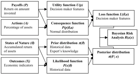
2.1 The Structure of the Decision Model
Figure 1 – The Structure of the Decision Model.
2.2 The Actions Set
In a portfolio selection problem, a common situation is for an investor to have a fixed budget and to have to decide on the asset allocation within this budget constraint. In this study, the actions set will consist of a vector of the percentages of each asset to be invested. For n assets the actions set can be represented by:
A = {a1, a2 , ..., an} and 1
1
n
i i
a
= =
∑
(1)For example, suppose that the investor wants to invest his budget in three types of assets, BOVESPA, DOW JONES and NASDAQ. This set will be represented by A = {a1, a2, a3}
where a1 + a2 + a3 = 1.
Figure 2 presents the graphic representation of the actions set in three dimensions. The investor can choose a point on this plane that corresponds to the percentage that will be invested in each kind of financial asset, a1, a2 and a3.
Figure 2 – Actions Set.
Payoffs (P)
Return on amount invested
Actions (A)
Percentage of assets
States of Nature (θ)
Accumulated return of assets
Outcomes (X)
Economic indicators
Utility function U(p)
Decision maker features
Consequence function P(p|θ,a)
Normal distribution
Prior distribution π(θ)
Historical data Expert’s knowledge
Likelihood function P(x|θ)
Historical data
Loss function L(θ,a)
Decision maker features
Posterior distribution
Philosophically, when one considers a decision theory background, the decision maker is allowed not to make a decision. This means that this decision maker “decided” “not to decide”, which in this particular case would mean not to invest. In a situation where the investor establishes that part of the budget ought not to be invested, or used as a “savings” or as a reserve asset, it is enough to establish a new asset (action) which can represent this “non-investment” or an investment with very low risks and returns. Thus, this problem can be dealt with in a more general way. There are some situations where all assets offer a very high risk level, and perhaps reserving an amount not to be invested in risky assets is good way to deal with it. In this paper it has been considered that the set of actions has n-1 degrees of freedom, due to the restriction that the sum of the percentage of the assets should be equal to one.
2.3 The Payoffs Set
The payoffs set of this decision problem is the return on the amount invested. Let rt be the
return of an action at the period t, and Vt the value of the asset on period t, then:
1 1 t t t t V V r V − − −
= (2)
Let Rt be the accumulated return for t periods, then:
1 (1 ) t t i i R r =
=
∏
+ (3)As each asset has a different return, the accumulated return is a vector with one element for each financial asset, so R = {Rt1, Rt2, ..., Rtn}.
The evaluation of the payoffs set is obtained by the accumulated return rate on each investment in t periods after the investment date, multiplied by the value invested. Let B be the budget to be invested, then the value of payoffs is obtained by the following expression: 1 ( ) n i ti i
P B a R
=
= ⋅
∑
⋅ (4)2.4 States of Nature Set
Nature states are represented by a vector with the accumulated return rates for each asset where the budget can be invested for the next t periods. In other words, future returns are unknown. The uncertainty contained in this element is what motivates the development of this decision model. The vector of states of nature is represented in Equation (5).
Accumulated returns of n assets can be represented by a set of n continuous random
variables. Although this set can be modeled by a joint probability distribution, there is a need for a representative sample to estimate the prior distribution and likelihood function.
Therefore, in some situations it is more appropriate to create categories based on n
continuous random variables because of the limited amount of data. This space can be defined as a set of discrete random variables.
{
1, 2,..., n}
It is important to detach the existing difference among the set of states of nature, θ, and of payoffs, P. It is known that the market will define the states of nature and the investor will obtain a certain return according to the decision made previously. In other words, θ will be represented by a vector with size n, and P will be a value obtained by the internal product among the percentage vector of assets, A, and the returns on those assets, R, for a certain time horizon.
2.5 Outcomes Set
The outcomes set can be based on a vector of economic indicators, for example, gross domestic product, official interest rate, the rate of inflation and other parameters used as indicators. Let k be the number of indicators that need to be observed, then:
{
1, 2,..., k}
X = x x x (6)
This set can also be treated as discrete in the same way as the states of nature set.
2.6 Consequence Function
The consequence function is a probabilistic mechanism that seeks to estimate the probability of having the payoff P given that a certain decision has been made and one specific state of nature has taken place.
The value of payoffs is regarded as a weighted sum of accumulated returns by percentages of investments in each asset as defined by Equation (4). In order to try to represent the consequence function, it can be assumed that this function is a weighted sum of probability distributions, and each probability distribution represents a conditional probability of accumulated return given a state of nature. The percentage of investment in each asset is the weight of these distributions.
1
( | , ) ( | ) n
i i
P p θ a a P p θ
=
=
∑
⋅ (7)Based on statistical analysis of real data, it assumed that these distributions can be modelled by normal distribution.
Let respectively µθ i and σθ i be the average and the standard deviation estimated for each
asset i conditioned to the state of nature θ, and then the consequence function will be:
1
( | , ) ( , , )
n
i i i
i
P p θ a a Normal p µ σθ θ
=
=
∑
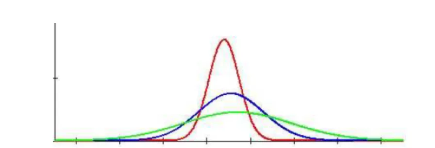
⋅ (8)Where, Normal p( , , )µ σ denotes the normal density function with the mean µ and standard deviation σ.
Figure 3 – Normal Distributions for Consequence Functions, P p( | , )θ a .
2.7 Others Elements of the Decision Model
The prior distribution around states of nature, π(θ), can be estimated directly from the relative frequency of the series of historical accumulated index returns, or obtainable through expert’s knowledge. Lins & Souza (2001) present a protocol for the elicitation of prior distributions.
The likelihood function, P(x|θ), characterizes the probability of occurrence of certain
outcomes, given that a state of nature will happen in m following periods. This function
represents a communication channel between observations and nature, and it can be obtained from historical data which associates the observations and the states of nature. Assuming that the observations and the states of the nature are defined as discrete, this function will be a vector with a dimension (k x n), where k is the number of observations and n the number of states of nature.
The use of decision rules in this problem can be difficult due to the possibly large number of rules needed to analyze the problem. Therefore the use of the extensive method is recommended, where for each observation there is a recommendation for action.
Utility functions are used to measure the value given by the decision maker to the accumulated return on his portfolio in a certain period, that is, the utility is measured against the payoffs. This function can assume different formats for different investors and for the same investor in different periods. Through this function it can be observed if the investor is averse, prone or neutral to risk.
The loss function represents the loss arising from a decision made and the occurrence of a state of nature. It is measured by the negative result of the expected utility and it is denoted by L(θ,a). Thus:
( , ) ( ) ( | , ) p
Lθ a = −
∫
U p P p⋅ θ a dp (10)Based on the concept that risk means the expected value of a loss, the risk of an action given that x occurred will be obtained by
( ) ( , ) ( | ) ( ) a
r x L a P x
θ θ θ π θ
=
∑
⋅ ⋅ (11)The action chosen will be the one that minimizes ra(x) for a given observation. The value of
ra(x) shown in Equation (11) is the Bayes’ risk of this decision rule. This kind of decision
rule will incorporate a prior distribution about nature and also the negative result of the expected utility, represented by the loss function, giving an alternative that will minimize risk of losses. This makes it possible to observe some environmental characteristics and use them to choose an action that minimizes risk of losses. This approach is widely used in several applications and Dale (1991) describes several applications in Decision Theory.
3. Case Study
Using real data from financial market indices and asset indexes from January 1998 to June 2005 collected monthly, the decision problem is how much to invest in BOVESPA, DOW JONES and NASDAQ assets for the six months period from July 2005.
3.1 Actions Set
The actions set of a portfolio selection problem with three assets, ideally should be represented by space a1 + a2 + a3 = 1 as shown in Figure 1. However, due to computational complexity,
some points of this space were selected in order to simplify the computational effort needed. Otherwise, non-linear programming is necessary to find the optimal solution of this problem.
7 points of the actions space were selected to represent the actions set. These actions can be represented in the table below, and each value represents how much of the budget will be invested in each asset.
Table 1 – Actions Set.
a1 a2 a3
A0 1 0 0
A1 0 1 0
A2 0 0 1
A3 1/3 1/3 1/3
A4 1/2 1/4 1/4
A5 1/4 1/2 1/4
3.2 Payoffs Set
It is assumed that the investor will invest an amount of R$ 100,000.00, and the next six months of accumulated returns will belong to the range of the normal distribution limits of the consequence function. Although the limits of the normal distribution are (-∞, ∞), the limits considered in this case study were narrowed to reduce the computational effort.
The limits used were [0.4; 2], then the range of the payoffs is P = [40,000.00; 200,000.00]. Table 2 presents the descriptive statistics of accumulated returns over six months on assets in BOVESPA, DOW JONES and NASDAQ.
The data from the Brazilian financial market for this case study is based on 90 monthly index records from January 1998 to June 2005. Based on Equation (2), this data set results in 89 monthly returns. The accumulated return for the period of six months is considered.
Based on Equation (3) we have t = 6. For example, the first observation of Rt1 was
computed based on the accumulated return (t = 6) of the six first months, the second
observation of Rt1 was computed based on the return from the second to seventh month,
etc. There are 84 observations of the accumulated returns because there is an overlap of 5 months.
Table 2 – Descriptive Statistics of Accumulated Return.
Accumulated Return
N Mean Standard
Deviation Minimum Maximum
Rt1 84 1.100231 0.279246 0.551817 1.714154
Rt2 84 1.017122 0.102458 0.729719 1.255703
Rt3 84 1.030471 0.254115 0.500953 1.714859
3.3 States of Nature
The states of nature set of this case study is considered to be a discrete set, where the accumulated return over six months was evaluated. If the accumulated return is greater than 100% for an asset, then value 1 is assigned to this asset and 0 otherwise. For a three assets problem, we have a combination of eight possible situations.
The states of nature set is represented by a vector with three coordinates where each coordinate is presented in binary form, θ = θ1 x θ2 x θ3. This set will be represented by a set
of eight elements, where θ0=[0,0,0]; θ1=[0,0,1]; θ2=[0,1,0]; θ3=[0,1,1]; θ4=[1,0,0];
θ5=[1,0,1]; θ6=[1,1,0]; θ7=[1,1,1].
Table 3 – Frequency table of States of Nature.
Count Percent θ0 24 28.91566
θ1 1 1.20482
θ2 4 4.81928
θ3 4 4.81928
θ4 7 8.43373
θ5 5 6.02410
θ6 8 9.63855
θ7 30 36.14458
In Figure 4 we show the dispersion of the states of nature over time.
Figure 4 – Scatterplot of States of Nature.
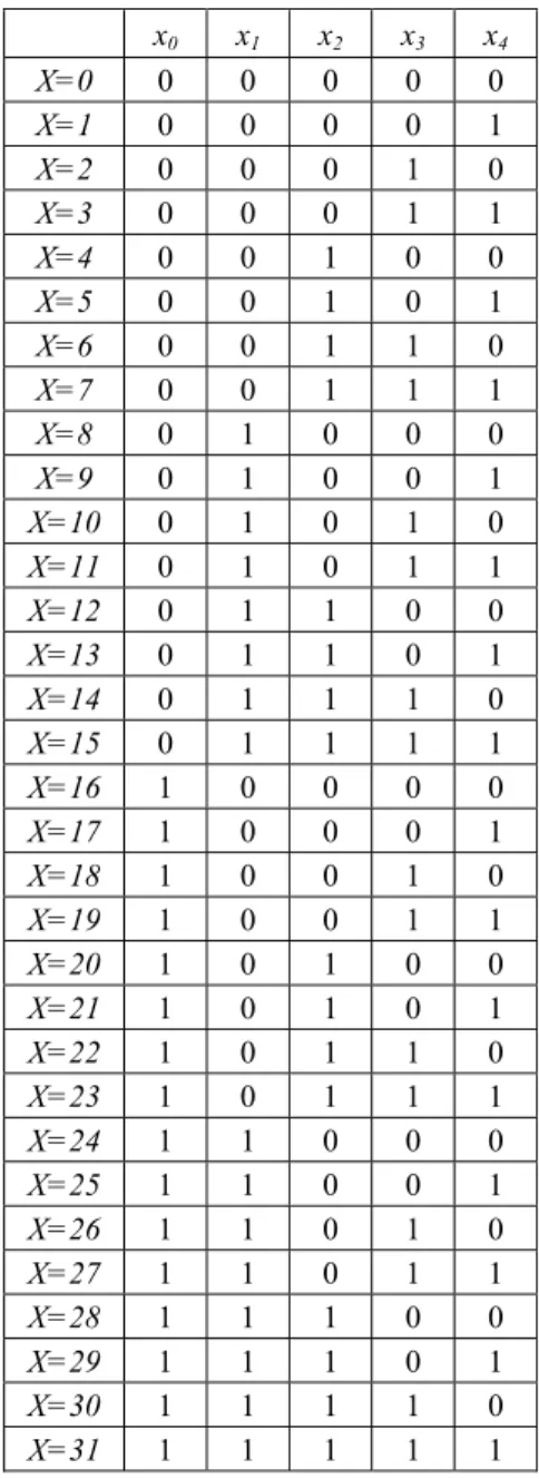
3.4 Outcomes Set
The outcomes set is defined by the indexes X = {x0, x1, x2, x3, x4}, according to the
definitions below:
• x0 will be 1 if the (monthly) Brazilian gross domestic product has a positive change
and 0 otherwise;
• x1 will be 1 if the (monthly) official Brazilian interest rate has a negative change and 0
otherwise;
• x2 will be 1 if (monthly) Brazilian inflation has a negative change and 0 otherwise;
• x3 will be 1 if the official (monthly) United States interest rate has a negative change
and 0 otherwise;
• x4 will be 1 if (monthly) United States inflation has a negative change and 0 otherwise.
Table 4 – Combination of Observations Set.
x0 x1 x2 x3 x4
X=0 0 0 0 0 0
X=1 0 0 0 0 1
X=2 0 0 0 1 0
X=3 0 0 0 1 1
X=4 0 0 1 0 0
X=5 0 0 1 0 1
X=6 0 0 1 1 0
X=7 0 0 1 1 1
X=8 0 1 0 0 0
X=9 0 1 0 0 1
X=10 0 1 0 1 0
X=11 0 1 0 1 1
X=12 0 1 1 0 0
X=13 0 1 1 0 1
X=14 0 1 1 1 0
X=15 0 1 1 1 1
X=16 1 0 0 0 0
X=17 1 0 0 0 1
X=18 1 0 0 1 0
X=19 1 0 0 1 1
X=20 1 0 1 0 0
X=21 1 0 1 0 1
X=22 1 0 1 1 0
X=23 1 0 1 1 1
X=24 1 1 0 0 0
X=25 1 1 0 0 1
X=26 1 1 0 1 0
X=27 1 1 0 1 1
X=28 1 1 1 0 0
X=29 1 1 1 0 1
X=30 1 1 1 1 0
X=31 1 1 1 1 1
The histogram of the frequencies and number of observations and dispersion of this element over time is presented in Figure 5.
Observations 2, 7, 11, 14, 15, 19, 21, 26, 27, 29 did not have any occurrences and were excluded from analysis.
frequent outcome. X = 12 means that the official Brazilian interest rate and Brazilian inflation had a positive change in that month and the Brazilian gross domestic product, the official United States interest rate and United States inflation had a negative change. The scatterplot of outcomes in Figure 5 shows the time series of these observations.
Figure 5 – Histogram and Scatterplot of Outcomes.
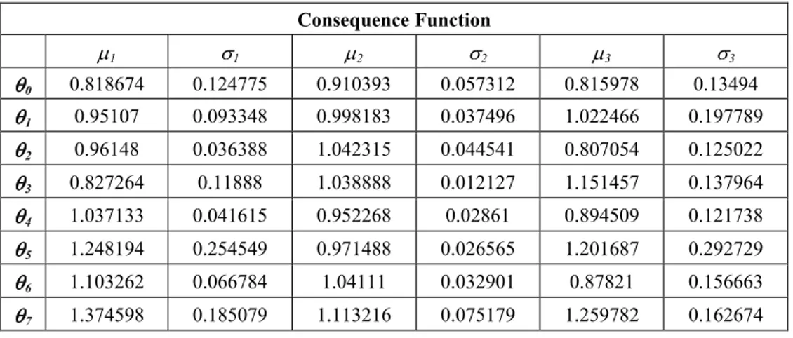
3.5 Consequence Function
Based on the normality hypothesis for accumulated returns in order to estimate the consequence function, the values of the average and standard deviations were estimated for each state of nature, as shown in Table 5 and Figure 6.
The consequence function is assumed by hypothesis to have the behavior of Equation (8). There is a probability distribution that is a mixture of a set of n normal distributions weighted by the percentage of investment in each asset. This distribution is conditioned to percentages of assets and the occurrence of a state of nature. For example, in the first row of Table 5 the state of nature θ0 is considered, then a filter of the occurrence of this state needs be applied
(24 occurrences in this case study). Similarly, a normal distribution fitting for each asset should be carried out in order to estimate the mean and standard deviation for each asset.
Table 5 – Mean and Standard Deviation Estimated for Accumulated Return for Each Asset.
Consequence Function
µ1 σ1 µ2 σ2 µ3 σ3
θ0 0.818674 0.124775 0.910393 0.057312 0.815978 0.13494
θ1 0.95107 0.093348 0.998183 0.037496 1.022466 0.197789
θ2 0.96148 0.036388 1.042315 0.044541 0.807054 0.125022
θ3 0.827264 0.11888 1.038888 0.012127 1.151457 0.137964
θ4 1.037133 0.041615 0.952268 0.02861 0.894509 0.121738
θ5 1.248194 0.254549 0.971488 0.026565 1.201687 0.292729
θ6 1.103262 0.066784 1.04111 0.032901 0.87821 0.156663
Figure 6 – Normal Distributions of Consequence Function, ( | , )P p θ a .
3.6 States of Nature Prior Distribution
The prior distribution was obtained through the relative frequency of each state of nature in the period from January 1998 to June 2005.
Although there are other ways to obtain the prior distributions of states of nature, the relative frequency of the states of nature was used in this case study as presented in Table 3.
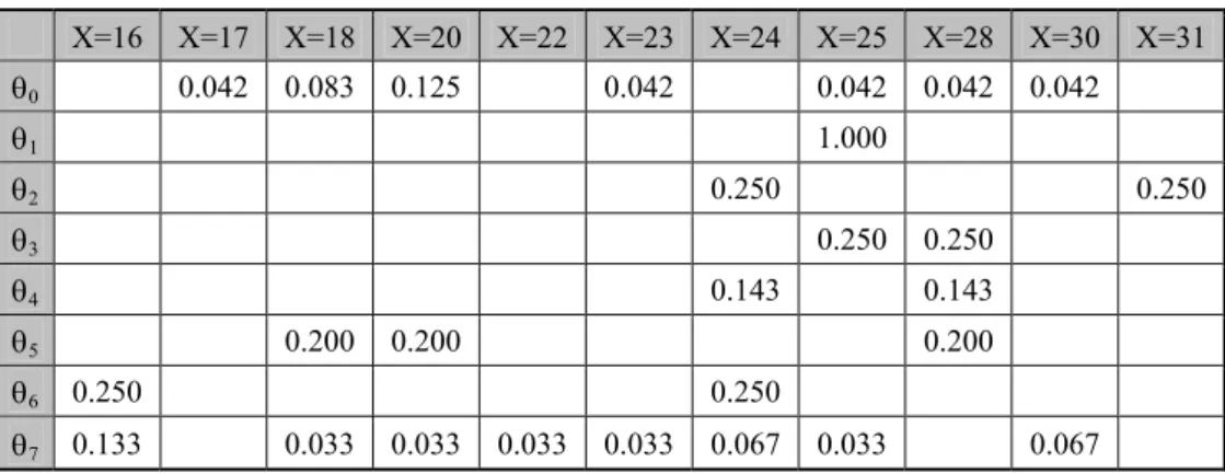
3.7 Likelihood Function
The likelihood function, P(x|θ), was obtained by the relative frequency of the last
occurrences associating states of nature and outcomes. Table 6 displays estimated values, where empty cells represent value zero. For example, P(X=1|θ0)=0.042 means that in the past 4.2% of the outcomes when θ0 occurred were X=1.
Table 6 – Likelihood Function.
X=0 X=1 X=3 X=4 X=5 X=6 X=8 X=9 X=10 X=12 X=13
θ1 0.042 0.042 0.083 0.125 0.292
θ1
θ2 0.250 0.250
θ3 0.250 0.250
θ4 0.143 0.143 0.286 0.143
θ5 0.400
θ6 0.125 0.125 0.125 0.125
X=16 X=17 X=18 X=20 X=22 X=23 X=24 X=25 X=28 X=30 X=31
θ0 0.042 0.083 0.125 0.042 0.042 0.042 0.042
θ1 1.000
θ2 0.250 0.250
θ3 0.250 0.250
θ4 0.143 0.143
θ5 0.200 0.200 0.200
θ6 0.250 0.250
θ7 0.133 0.033 0.033 0.033 0.033 0.067 0.033 0.067
3.8 Utility Function
The utility function used in this study case is a linear utility function, parameterized with the payoffs limits [0.4; 2], in order to rescale the utility into [0; 1]. Thus:
0.4 ( )
2 0.4 p
U p = −
− (12)
3.9 Loss Function and Bayesian Risk Analysis
With the Loss Function defined in (10) and Bayesian Risk in (11) we obtain the results in Table 7. In the first row, we have the risk of actions conditioned to the outcome X=0. For
example, rA0(X=0) = -0.0255. This means that if X=0 (the Brazilian Gross Domestic
Product has a negative change and the Brazilian interest rate, Brazilian inflation, the United States interest rate and United States inflation have a positive change), the expected loss is -0.0255. For the outcome X=0, A0 is the action with the minimum risk, in other
words, this action has the lowest value in the first row. This analysis can be applied to all outcomes in Table 7. The actions with the minimum risk conditioned for each outcome are highlighted in Table 7.
Table 7 – Bayesian Risk Analysis.
A0 A1 A2 A3 A4 A5 A6
X=0 -0.0255 -0.0190 -0.0222 -0.0222 -0.0230 -0.0214 -0.0222
X=1 -0.0032 -0.0039 -0.0032 -0.0034 -0.0033 -0.0035 -0.0033
X=3 -0.0053 -0.0048 -0.0036 -0.0046 -0.0048 -0.0046 -0.0043
X=4 -0.0265 -0.0222 -0.0223 -0.0237 -0.0244 -0.0233 -0.0233
X=5 -0.0075 -0.0055 -0.0066 -0.0065 -0.0068 -0.0063 -0.0066
X=6 -0.0116 -0.0125 -0.0098 -0.0113 -0.0114 -0.0116 -0.0109
X=8 -0.0550 -0.0517 -0.0533 -0.0533 -0.0538 -0.0529 -0.0533
X=10 -0.0075 -0.0055 -0.0066 -0.0065 -0.0068 -0.0063 -0.0066 X=12 -0.0777 -0.0733 -0.0757 -0.0756 -0.0761 -0.0750 -0.0756
X=13 -0.0128 -0.0103 -0.0102 -0.0111 -0.0115 -0.0109 -0.0109 X=16 -0.0408 -0.0318 -0.0339 -0.0355 -0.0368 -0.0346 -0.0351
X=17 -0.0032 -0.0039 -0.0032 -0.0034 -0.0033 -0.0035 -0.0033 X=18 -0.0202 -0.0175 -0.0189 -0.0188 -0,0192 -0.0185 -0.0188 X=19 0.0000 0.0000 0.0000 0.0000 0.0000 0.0000 0.0000
X=20 -0.0233 -0.0213 -0.0220 -0.0222 -0.0225 -0.0220 -0.0222 X=21 0.0000 0.0000 0.0000 0.0000 0.0000 0.0000 0.0000
X=22 -0.0075 -0.0055 -0.0066 -0.0065 -0.0068 -0.0063 -0.0066
X=23 -0.0107 -0.0094 -0.0098 -0.0099 -0.0101 -0.0098 -0.0099 X=24 -0.0328 -0.0280 -0.0258 -0.0289 -0.0299 -0.0287 -0.0281 X=25 -0.0205 -0.0223 -0.0244 -0.0224 -0.0219 -0.0224 -0.0229
X=28 -0.0179 -0.0190 -0.0212 -0.0194 -0.0190 -0.0193 -0.0198 X=30 -0.0184 -0.0150 -0.0166 -0.0167 -0.0171 -0.0163 -0.0167
X=31 -0.0042 -0.0048 -0.0031 -0.0040 -0.0041 -0.0042 -0.0038
With the decision model built in this study, it was possible to conclude that all budgets might be invested in only one asset. If we have a scenario where X={x0, x3, x4, x5, x8, x9, x10, x12, x13,
x16, x18, x20, x22, x23, x24, x30}, then the best portfolio of investments would be in BOVESPA,
where A0 is preferable. On the X = {x1, x6, x17, x31} scenario the best portfolio would be in
DOW JONES, where A1 is preferable. And for the scenario X= {x25, x28} the best portfolio
would be in NASDAQ, where A2 is preferable. The best solutions in this case study are to be
found only in A0, A1 and A2.
4. Conclusions
We conclude that this model is quite appropriate for financial market use. The probability distributions can be updated and they will incorporate more information into the model in future decisions. Surprisingly the actions that were compiled for more than one asset were not recommended by the model. We believe this occurs due to Bayesian Risk Analysis being based on the value of the losses expected. Perhaps a new element of variance of the portfolios can be incorporated into the model in a future study in order to enable us to answer this question.
Acknowledgements
References
(1) Abdelaziz, F.B.; Aouni, B. & Fayedh, R.E. (2007). Multi-objective stochastic
programming for portfolio selection. European Journal of Operational Research, 177, 1811-1823.
(2) Ballestero, E.; Gunther, M.; Pla-Santamaria, D. & Stummer C. (2007). Portfolio
selection under strict uncertainty: A multi-criteria methodology and its application to
the Frankfurt and Vienna Stock Exchanges. European Journal of Operational Research,
181, 1476-1487.
(3) Berger, J.O. (1985). Statistical Decision Theory and Bayesian Analysis.
Springer-Verlag, Berlin.
(4) Crama, Y. & Schyns, M. (2003). Simulated annealing for complex portfolio selection
problems. European Journal of Operational Research, 150, 546-571.
(5) Dale, I.A. (1991). A history of inverse probability: From Thomas Bayes to Karl
Pearson. Springer-Verlag.
(6) Deng, X. -T.; Li, Z.-F. & Wang, S.-Y. (2005). A minimax portfolio selection strategy with equilibrium. European Journal of Operational Research, 166, 278-292.
(7) Ehrgott, M.; Klamroth, K. & Schwehm, C. (2004). An MCDM approach to portfolio
optimization. European Journal of Operational Research, 155, 752-770.
(8) Lin, C.-C. & Liu, Y.-T. (2007). Genetic algorithms for portfolio selection problems
with minimum transaction lots. European Journal of Operational Research, In Press,
Corrected Proof, Available online 11 January 2007.
(9) Lins, G.C.N. & Souza, F.M.C. (2001). A Protocol for the Elicitation of Prior
Distributions. In: 2nd International Symposium on Imprecise Probabilities and Their
Applications, Ithaca, New York.
(10) Mao, J.C.T. & Särndal, E. (1966). A Decision Theory Approach to Portfolio Selection. Management Science, 12(8), B323-B333.
(11) Markowitz, H. (1952). Portfolio selection. Journal of Finance, 7, 77-91.
(12) Markowitz, H.M., (1991). Foundations of portfolio theory. Journal of Finance, 46(2), 469-478.
(13) Prakash, A.J.; Chang, C.-H. & Pactwa, T.E. (2003). Selecting a portfolio with skewness:
Recent evidence from US, European, and Latin American equity markets. Journal of
Banking & Finance, 27, 1375-1390.
(14) Rubinstein, M.(2002). Markowitz’s “Portfolio Selection”: A Fifty-Year Retrospective.
The Journal of Finance, 62(3), 1041-1045.
(15) Soyer, R. & Tanyeri, K. (2006). Bayesian portfolio selection with multi-variate random variance models. European Journal of Operational Research, 171, 977-990.
(16) Young, M.R. (1998). A Minimax Portfolio Selection Rule with Linear Programming