Braz. J. Chem. Eng. vol.19 número4

ISSN 0104-6632 Printed in Brazil

Vol. 19, No. 04, pp. 467 - 474, October - December 2002

of Chemical

Engineering

AN MILP FORMULATION FOR THE SCHEDULING

OF MULTIPRODUCT PIPELINE SYSTEMS

R.Rejowski Jr. and J.M.Pinto

Department of Chemical Engineering, University of São Paulo, USP, Av. Prof. Luciano Gualberto, Travessa 3, 380, 05508-900, São Paulo - SP, Brazil.

E-mail: [email protected] E-mail: [email protected]

(Received: March 5, 2002 ; Accepted: May 27, 2002)

Abstract - Pipelines provide an economic mode of fluid transportation for petroleum systems, specially when large amounts of these products have to be pumped for large distances. The system discussed in this paper is composed of a petroleum refinery, a multiproduct pipeline connected to several depots and the corresponding consumer markets that receive large amounts of gasoline, diesel, LPG and aviation fuel. An MILP optimization model that is based on a convex-hull formulation is proposed for the scheduling system. The model must satisfy all the operational constraints, such as mass balances, distribution constraints and product demands. Results generated include the inventory levels at all locations, the distribution of products between the depots and the best ordering of products in the pipeline.

Keywords: pipeline, scheduling, logistics, distribution planning, optimization.

INTRODUCTION

Planning and scheduling activities related to product distribution have been receiving growing attention since the past decade. Every company should focus on attending all its client requirements at the lowest possible cost. As a matter of fact, transportation costs had already surpassed 400 billions dollars in the early eighties (Bodin et al., 1983).

Petroleum products can be transported by road, railroad, vessels and pipeline. The latter has usually been utilized for crude oil transportation from terminals to refineries (Mas and Pinto, 2002).

Pipeline transportation is the most reliable and economical mode for large amounts of liquid and gaseous product. It differs from the remaining modes, since it can operate continuously (Sasikumar et al., 1997). For the past forty years, pipelines have mainly been utilized by the petroleum industry for transportation of petroleum and its derivatives.

Shobrys and White (2000) and Katzer et al. (2000) mention the importance of MINLP models for the programming of operations in oil refineries because of the inherent nonlinearities of chemical processes and the possibility of representing discontinuous functions and operational decisions. Pinto et al. (2000) present optimization models for planning and scheduling in petroleum refineries. Shah (1996) presents an MILP for crude oil scheduling in a system consisting of a port connected to a refinery by a pipeline. Moro and Pinto (1998) studied the efficiency of an MILP for the allocation of crude oil to tanks.

crude oil and petroleum products in complexes with multiple pipelines.

The system considered in this work is composed of a petroleum refinery, a multiproduct pipeline and several depots that are connected to local consumer markets. Large amounts of oil derivatives that are generated in the refinery must be pumped for long distances until they reach their destinations. The major obstacles faced in these operations are concerned with the satisfaction of product demands by the various consumer markets and the large variation of the same within a small time horizon. Moreover, product sequencing is subject to constraints, which further complicate the generation of optimal schedules for system operation.

A mixed-integer linear programming model is proposed for the simultaneous optimization of systems with multiple depots. This model must satisfy all the operational constraints, such as mass balances, distribution constraints, product demands and storage requirements. It relies on a uniform discrete time representation and a logical formulation generated from linear disjunctions, which are modeled by a convex-hull formulation.

The results generated by this model are the inventory level profiles for all products at the refinery, in all pipeline segments and at the depots along the distribution horizon. The formulation is tested and compared for systems containing up to three depots. This approach is successfully tested in an example that is based on a real-world system that transports four products, which must feed five distribution depots in the southeastern and central regions, from the REPLAN refinery in Paulínia (SP, Brazil). The model was able to find a real-optimal solution for a three-day time horizon.

PROBLEM DEFINITION

A refinery must distribute P petroleum products between D depots connected to a single pipeline, which is divided into D segments. The depots have to satisfy requirements determined by local consumer markets. The pipeline system is shown in Figure 1. Note that a segment can be defined as the part of the pipeline between two consecutive storage centers (refinery and depots).

In the refinery as well as in the distribution depots there may be more than one tank for each product. However, at most one tank must be connected to the pipeline at any time.

Product transfer must satisfy volume and maximum flow rate constraints in the pipeline. There

are also forbidden sequences of products in the pipeline. Operation of multiproduct pipelines has a unique feature, product contamination. Although pipelines provide a safe mode of transportation, product contamination is inevitable and it occurs at the interface of two miscible products. Techo and Holbrook (1974) mention that the costs of this are usually very high.

The depots must control their inventory levels and satisfy product demands imposed by the local consumer markets. Demands must be matched according to inventory levels in the refinery and to pipeline capacity. As products are transported by only one pipeline and very large distances must be covered, it is critical that the correct decisions be made, since delays of several days may occur.

Management of the distribution depots basically requires one major decision in each time period, the transfer of products to the consumer markets. Constraints are imposed by the lower and upper bounds on tank capacities, the transportation time and the timing of the operations of unloading from the pipeline. Operating costs include inventory costs in the refinery as well as in the depots, pumping costs and finally transition costs between different products inside the pipeline. Inventory costs are related to the stored amounts of products at all locations and to the time these remain in the tanks for all systems. Pumping costs are proportional to the amount of each product sent by the refinery and to the distance it covers in the pipeline. Pumping cost coefficients depend on the distances of the depots from the refinery. The most challenging cost term is that which accounts for transition costs. There is one cost for each pair of products that accounts for losses as well as interface reprocessing at each of the distribution depots.

Due to the large number of decisions concerning the system, only a systematic and simultaneous approach may be suitable for this operation.

OPTIMIZATION MODEL

The present mathematical model must represent the correct operational mode of the refinery, the pipeline segments and finally the local depots. The most challenging feature is that product transfer can be temporarily interrupted during the time horizon. Due to this aspect, the representation used for the pipeline system is based on Figure 2.

enters segment d at time k, the content of the first pack in that segment is transferred to the next pack. The same occurs to all packs in the same segment. Consequently, the same amount of product must either leave the segment (VODp,d,k) or be transferred to segment d+1 (VOTp,d+1,k). If no product enters d at time k (VOTp,d,k = 0 ), then all packs keep the same content.

The main assumptions are as follows: (1) All products have constant densities; (2) The production rate and demands are known during the time horizon; (3) All tanks for each product have aggregated capacities; (4) At most one tank at the refinery and at all depots can be connected to the pipeline at any time; and (5) The pipeline segments are always completely filled.

Figure 1: Distribution Pipeline System

Figure 2: Generic Pipeline Segment

Mathematical Formulation

The tanks at the refinery are modeled by constraints (1) to (3). Equations (1) represent the volumetric balances for all products at any time interval, whereas the minimum and maximum capacities are imposed in constraint (2). The pipeline feed (VORp,k) is a function of the volumetric parameter U and binary variable XRp,k, which is 1 if the refinery feeds the pipeline with product p at time k, according to equation (3).

p, k p p, k p, k

VR =VRZERO +RP ×δ −VOR

(1a)

∀p, k=1

VRp, k=VRp, k 1 RPp, k− + ×δ −VORp, k

(1b)

∀p, k=2,…,K

VRMINp, k≤VRp, k≤VRMAXp, k ∀p, k (2)

VORp, k= ×U XRp, k ∀p, k (3)

there is a transfer of p at time k (XRp,k = 1 and from (5) XS1,k = 1), constraint (8) activates XVp,1,1,k; note that the other transfers between packs (l=2, …, L) are activated in a chain effect through (9). Otherwise (XRp,k = XS1,k = 0), the product contained in every pack l at k remains inside it, as imposed by (10). The same logic follows for all the remaining segments.

Vp,d, l, k=XVp,d,l, k U× ∀ p,d, l, k (4)

P

XRp, k XSd, k p 1

= =

∑

XSd, k≤1 ∀ d, k (6)

P

XVp,d,l, k 1 p 1

= =

∑

XVp,d, l, k≥XRp, k ∀ p, k, d=1, l=1 (8)

XVp,d, l, k≥XVZEROp, d,l 1 [1 XSd, k]− − −

(9a)

∀ p, d, l=2,…,L, k=1

XVp,d, l, k≥XVp,d,l 1, k 1 [1 XSd, k]− − − −

(9b)

∀ p, d, l=2,…,L, k=2,…,K

XVp,d, l, k≥XVZEROp, d,l−XSd, k

(10a)

∀ p, d, l, k=1

XVp,d, l, k≥XVp,d,l, k 1 XSd, k− −

(10b)

∀ p, d, l, k=2,…,K

P

[XDp,d, k XTp,d 1, k] XSd, k p 1

+ + =

=

∑

(11)

∀ k, d<D

XDp,d, k XTp,d 1, k

XVZEROp,d, l [1 XSd, k]

+ + ≥

≥ − − (12a)

∀ p, d<D, l= L, k=1 XDp,d, k XTp, d 1, k

XVp,d,l, k 1 [1 XSd, k]

+ + ≥

≥ − − − (12b)

∀ p, d<D, l= L, k=2,…,K

VOTp, d, k=XTp, d, k U× ∀ p,d>1, k (13)

VOTp, d, k= ∀0 p, d=1, k (14)

Constraints for segment d (d ≠ D) are the same as the ones for the first segment with the exception of constraints (5) and (8), which are replaced respectively by constraints (15) and (16). Variable VOTp,d,k replaces VORp,k because this segment d is fed by its predecessor d-1.

P

XTp, d, k XSd, k p 1

= =

∑

XVp,d, l, k≥XTp, d, k ∀ p,d>1, l=1, k (16)

Constraints for the last segment (d = D) are the same as the ones for a generic middle segment with the exception of constraints (11) and (12), which are replaced respectively by constraints (17) and (18).

P

p, d, k d, k p 1

XD XS

= =

∑

p, d, k p, d, l d, k XD ≥XVZERO − −[1 XS ]

(18a)

∀ p, d=D, l= L, k=1

p, d, k p, d, l, k 1 d, k

XD ≥XV − − −[1 XS ]

(18b)

∀ p, d=D, l= L, k=2,…,K

Pinto and Grossmann (1998) and Pinto et al. (2000) describe many approaches for modeling transitions in scheduling systems. Constraints (20) and (21) model transitions for the present case. Note that it is only necessary to verify transitions between two consecutive packs of each segment d (the first and second were selected).

TYp, p ', d, k≥XVp, d,1, k+XVp ', d, 2, k 1−

(19) {∀p, p’, d|∈TSp,p’}, ∀ k

p, p ', d, k

TY =0 {∀p ,p’, d|∈FSp,p’}, ∀ k (20)

VDp,d, k VDZEROp,d XDp,d, k U VOMp,d, k

= +

+ × − (21)

∀ p , d, k=1

VDp,d, k VDp, d, k 1

XDp,d, k U VOMp, d, k

= − +

+ × − (22)

∀ p, d, k=2,…,K

p, d, k p, d, k p, d, k

VDMIN VD

VDMAX

≤ ≤

≤ (23)

∀ p, d, k

VOMp,d, k≤UMp,d, k ∀ p ,d ,k (24)

K

p, d, k p, d k 1

VOM DEM

= =

∑

Objective Function

The overall operational cost is given by equation (26). The terms in brackets represent inventory costs at the refinery and depots, respectively. The third and fourth terms refer to pumping costs and product transitions.

P K P D K

C CERp VRp, k CEDp, d VDp, d, k

p 1k 1 p 1d 1k 1

 

 

= _ × + × _δ +

= = = = =

 



∑ ∑

∑ ∑ ∑

(26)

P D K P P D K

CPp, d, k VODp,d, k CONTACTp, p ' TYp, p ',d, k

p 1d 1k 1 p 1p ' 1d 1k 1

+ × + ×

= = = = = = =

∑ ∑ ∑

∑ ∑ ∑ ∑

EXAMPLE

An example composed of fifteen time intervals is presented in this section. Data for this example, including number of products and depots and the set of forbidden product sequences, are given in Table 1. GAMS modeling language (Brooke et al., 2000) was used to implement the MILP model that was solved with CPLEX (Ilog , 1999).

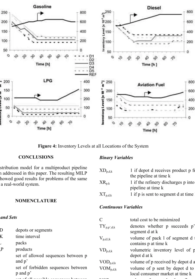
Figure 3 illustrates the production profile at the refinery for the entire time horizon, whereas Figure 4

shows the inventory levels for the refinery and all depots for each of the products. A scenario of intensive production by the refinery is represented. Note that the inventory levels at all depots are minimized as the demands are met during operation. Depots 3, 4 and 5 utilize the products that were inside the pipeline in order to satisfy the local consumer markets, while depots 1 and 2 require products from the refinery. Note that a three-day horizon time is scheduled. A 4.7% relative optimality gap was achieved.

Table 1: Data for Example

Product CERp

[$/m3.h]

CED p,d [$/m3.h]

RPp,k [m3/h]

CPp,d

[$/m3] FSp,q

Gasoline (1) 0.070 0.100 5 3.5/ 4.5/ 5.5/ 6.0/ 6.9 4.3

Diesel oil (2) 0.080 0.155 5 3.6/ 4.6/ 5.6/ 6.2/ 7.3 3.4

LPG (3) 0.095 0.200 5 3.8/ 4.8/ 5.8/ 6.8/ 7.9 3.2

Jet fuel (4) 0.090 0.170 5 3.7/ 4.7/ 5.7/ 6.1/ 7.0 2.3

VRZEROp [m3] VDZEROp,1 [m3] VDZEROp,2 [m3] Initial Content (d) [m3]

500, 520, 210, 515 190/ 180/ 50/ 120 230/ 210/ 65/ 140 d=1/ 75(p=1), 25(p=2)

VDZEROp,3 [m3] VDZEROp,4 [m3] VDZEROp,5 [m3] d=2/ 100(p=2)

200/ 180/ 60/ 190 240/ 180/ 60/ 190 190/ 180/ 60/ 170 d=3/ 50(p=1), 50(p=2)

DEMp,1 [m 3

] DEMp,2 [m

3

] DEMp,3 [m

3

] d=4/ 75(p=1), 25(p=2)

100/ 70/ 60/ 60 110/ 90/ 40/ 50 120/ 100/ 40/ 50 d=5/ 75(p=1)

DEMp,4 [m 3

]

120/ 80/ 0/ 50

DEMp,5 [m 3

]

150/ 100/ 20/ 50

VRMAXp/ VRMINp [m 3

]

1000/270; 1000/270; 300/100; 1000/270

Segment Capacity d [m3] (U) /UM [m3] Interval Duration (δ) [h]

Figure 4: Inventory Levels at all Locations of the System

CONCLUSIONS

A distribution model for a multiproduct pipeline has been addressed in this paper. The resulting MILP model showed good results for problems of the same scale as a real-world system.

NOMENCLATURE

Indices and Sets

d=1,…,D depots or segments k=1,…,K time interval l=1,…,L packs p=1,…,P products

ASp,p’ set of allowed sequences between p and p’

FSp,p’ set of forbidden sequences between p and p’

TSp,p’ set of all possible sequences between p and p’

Binary Variables

XDp,d,k 1 if depot d receives product p from the pipeline at time k

XRp,k 1 if the refinery discharges p into the pipeline at time k

XTp,d,k 1 if p is sent to segment d at time k

Continuous Variables

C total cost to be minimized

TYp,p’,d,k denotes whether p succeeds p’ in segment d at k

Vp,d,l,k volume of pack l of segment d that contains p at time k

VDp,d,k volumetric inventory level of p at depot d at k

VODp,d,k volume of p received by depot d at k VOMp,d,k volume of p sent by depot d to the

local consumer market at time k VORp,k volume of p sent by the refinery to

VOTp,d,k volume of p sent from segment d to d+1 at k

VRp,k volumetric inventory level of p at the refinery at k

XSd,k denotes whether segment d is under operation at k

XVp,d,l,k denotes whether pack l from segment d contains product p at time k

Parameters

CEDp,d inventory unit cost of p at depot d CERp inventory unit cost of p at the

refinery

CONTACTp,p’ transition cost from p to p’

CPp,d,k unit cost for pumping p to depot d at k

DEMp,d demand of p at consumer market supplied at depot d

RPp,k production rate of p at the refinery

U volume of packs

UMp,d,k upper bound on the volume of p sent by d at k

VDMAXp,d,k/ maximum/ minimum volumetric /VDMINp,d,k capacity of p at depot d at time k VDZEROp,d initial inventory level of p at depot d VRMAXp,k/ maximum / minimum volumetric /VRMINp,k capacity of p at the refinery at time k VRZEROp initial inventory level of p at the

refinery.

ACKNOWLEDGEMENTS

The authors would like to thank CAPES for its financial support and especially Petrobras Logistics Coordinator Marlise Fany Lehner.

REFERENCES

Bodin, L., Golden, B., Assad, A. and Ball, M. (1983). Routing and Scheduling of Vehicles and Crews. The State of the Art. Computers & Operations Research, 10 (2), 62.

Brooke, A., Kendrick, D. and Meeraus, A. A. (2000). GAMS - A User's Guide (Release 2.50). The Scientific Press. Redwood City, USA.

Ilog Corp. (1999). Ilog Cplex (6.5) User´s Manual. Gentilly, Cedex, France.

Katzer, J.R., Ramage, M.P. and Sapre, A.V. (2000). Petroleum Refining: Poised for Profound Changes. Chem. Eng. Prog., 96 (7), 41.

Mas, R. and Pinto, J.M. (2002). Mixed-Integer Optimization Techniques for Oil Supply in Distribution Complexes. Optimization and Engineering, accepted for publication.

Moro, L.F.L. and Pinto, J.M. (1998). A Mixed Integer Model for Short-Term Crude Oil Scheduling. AIChE 1998 Annual Meeting, Session 241, Miami Beach (FL).

Pinto, J.M. and Grossmann I.E. (1998). Assignment and Sequencing Models for the Scheduing of Process Systems. Annals of Operations Research, 81, 433.

Pinto, J.M., Joly, M. and Moro, L.F.L. (2000). Planning and Scheduling Models for Refinery Operations. Comput. Chem. Eng., 24, 2259. Raman, R. and Grossmann, I.E. (1994). Modeling

and Computational Techniques for Logic-Based Integer Programming. Comput. Chem Eng., 18 (7), 563.

Sasikumar, M., Prakash, P.R., Patil, S.M. and Ramani, S. (1997). Pipes: A Heuristic Search Model for Pipeline Schedule Generation. Knowledge Based Systems, 10 (3), 169.

Shah, N. (1996). Mathematical Programming Techniques for Crude Oil Scheduling. Comput. Chem. Eng., 20 (Suppl.), 1227.

Shobrys, D.E. and White, C.D. (2000). Planning, Scheduling and Control Systems: Why Can They Not Work Together. Comput. Chem. Eng., 24, 163.