Hidden Markov models applied to a subsequence of the Xylella fastidiosa

Hidden Markov models applied to a subsequence of the

Xylella fastidiosa

genome

Cibele Q. da-Silva

Universidade Federal de Minas Gerais, Departmento de Estatística, Belo Horizonte, MG, Brazil.

Abstract

Dependencies in DNA sequences are frequently modeled using Markov models. However, Markov chains cannot account for heterogeneity that may be present in different regions of the same DNA sequence. Hidden Markov models are more realistic than Markov models since they allow for the identification of heterogeneous regions of a

DNA sequence. In this study we present an application of hidden Markov models to a subsequence of theXylella

fastidiosa DNA data. We found that a three-state model provides a good description for the data considered.

Key words:DNA,Xylella fastidiosa, hidden Markov models.

Received: April 16, 2002; Accepted: June 26, 2003.

Introduction

The rate of sequence data generation in recent years has provided abundant opportunities not only for the devel-opment of new approaches to problems in computational biology but also for the exploration of the already known techniques on data that have never been analysed before.

The starting point in most data analysis consists of the use of well established methodology. As the analysis prog-ress, data particularities may require the development of specific tools that are more suitable to better describe and model the data. Creation of new methods requires deep un-derstanding of the current ones, especially when these methods are incredibly powerful and are not as known as they should be due to their mathematical and computational complexity. We consider that hidden Markov Models (HMM) exemplify this notion very well since although these models are not new, we believe that molecular biolo-gists are not aware of the possibilities that these models provide.

Our aim in this study is to discuss dependencies and heterogeneity in DNA data and how they can be appropri-ately accounted for by the use of HMM. We applied this

sort of model to a subsequence of theXylella fastidiosa(Xf)

genome as a way to suggest possible analysis for the whole genome.

According to Lambaiset al.(2000),Xylella fastidiosa

is a bacteria associated with diseases that cause tremendous losses in many economically important plants, including

citrus.Xylella fastidiosais the causal agent of Citrus

Varie-gated Chlorosis (CVC), a disease that affects all commer-cial sweet orange varieties and that represents a major concern to the Brazilian citrus industry. The plant pathogen attacks citrus fruits resulting in juiceless fruits of no

com-mercial value.Xylella fastidiosais the first plant pathogen

to have its genome (the total genetic information stored in the chromosomes of an organism) completely sequenced. In addition, it is probably the least previously studied of any organism for which the complete genome sequence is available.

Data sets generated by sequencing the entireXylella

fastidiosagenome pose new challenges since now biolo-gists need quantitative tools and statistical methods to help them to analyze sequences. Some recent publications about

Xylella fastidiosasignal the need not only for the applica-tion of current statistical methods available to analyse its sequenced data but also for statistical research to attack its

particularities. Chenet al. (2000) analysed sequenced data

from 16 strains ofXylella fastidiosaoriginating from nine

different hosts. They studied aspects such as sequence

het-erogeneity in the classification ofX. fastidiosaat the

sub-species level. The studies by Qinet al.(2000) and Mehtaet

al. (2001) are concerned with the evaluation of Xylella

fastidiosa genetic diversity isolated from diseased citrus and coffee in Brazil.

Due to the huge size of the datasets, statistical analy-ses for the whole genome of many organisms demand the use of high power state of the art computers. That may rep-resent a major problem since we do not have enough avail-able for this purpose.

www.sbg.org.br

Research Article

In this study we fit hidden Markov models to a dataset

of the bacteriaXylella fastidiosagenome. Model selection

is performed using the Bayesian Information Criterion (BIC) and Akaike’s Information Criteria (AIC). In section 2 we talk about dependencies in DNA data. In section 3 we discuss heterogeneity in DNA sequences. Hidden Markov Models are introduced in section 4. In section 5 we briefly introduce AIC and BIC for model selection. Phage lambda andXylella fastidiosadatasets are analysed in section 6.

Dependencies in DNA Data

An obvious first summary of a DNA sequence is just the distribution of the four base types. Although it would be convenient for mathematical modeling if the four bases were equally frequent, almost all empirical studies show an unequal distribution. That means that a simple independ-ence model for DNA sequindepend-ences have their uses, but only go a little way.

We need to take into account in a model the fact that neighboring bases in DNA sequences are not independent. According to Tavaré and Giddings (1989), associations be-tween adjacent bases will lead to associations bebe-tween more distant bases and an estimate of how far the relations extend may be found from Markov chain theory.

According to Weir (1996), Markov chain analyses are of use at the genome level, rather than at the level of an indi-vidual gene, since the last may involve very short se-quences that are not sufficient to demonstrate the presence of higher order chains. The same author observes that it is unlikely that the same Markov chain can describe the whole genome, and if a Markov chain has been fitted to a genome, no biological mechanism is implied, but useful questions can be answered. For example, the frequency of particular subsequences (words) can be predicted.

According to the website http://www.

accessexcellence.org/AE/AEC/, in genetic engineering it is common to use the many enzymes that are able to modify or join existing DNA molecules, or to aid in the synthesis of new DNA molecules. For example, the enzyme DNA poly-merase makes possible the attachment of two or more DNA molecules to one another. The enzyme DNA ligase breaks DNA molecules into fragments, while the so called restric-tion endonuclease enzyme (REE) funcrestric-tions by “scanning” the length of a DNA molecule. Once the REE encounters its particular specific recognition sequence (word), it will bond to the DNA molecule and cut it in a predictable and re-producible way. It is important to use Markov chains to help a biologist to estimate the expected number of frag-ments produced when a specific restriction enzyme is ap-plied to the genome.

Markov chains might describe DNA sequences in terms of their nucleotide composition,i.e., as a string of

let-ters from a four-letter alphabet, {A, C, G, T}. Let us denote

each one of the four base types asstates.We are going to

in-troduce some terminology and notation useful for Markov chains.

Generally speaking, for a given subject, let Xtdenote

the response on a categorical variable at time t, t = 0, 1, ..., T. The sequence (X0, X1, X2, ...) is an example of a

stochas-tic process, an indexed family of random variables. In this

paper Xtindicates the nucleotide at position t in the

se-quence.

Without invoking any biological mechanism, a

Markov chain of orderrimplies that the base present at

cer-tain position in a sequence depends only on the bases

pres-ent at the previousrpositions. In more formal grounds, a

stochastic process is arth-order Markov chain if, for allt,

the conditional distribution of Xt + 1, given X0, ..., Xt, is

iden-tical to the conditional distribution of Xt + 1, given Xt, ...,

Xt - r + 1. Given the states at the previousrtimes, the future

behavior of the chain is independent of the past behavior

before thosertimes. For a first-order Markov chain withI

possible states, the conditional probabilities

ηij(t) = Pr(X = j Xt _{t -1}= i) (1)

with i, j = 1, ..., I are calledtransition probabilities. The ex-tension for higher orders is immediate. Ifηij(t) does not

de-pend ont, the Markov chain is called homogeneous.

Statistical inference for Markov chain uses standard methods of categorical data analysis, such as log-linear models. Some useful references are Anderson and

Good-man (1957), Birch (1963), Bishopet al.(1975), McCullagh

and Nelder (1989), Agresti (1990), and Averyet al.(1999).

Heterogeneity in DNA Sequences

Markov chains and log-linear models are important tools to help us describe local properties of DNA se-quences. However, Markov chains cannot account for the heterogeneity that may be present in different regions of the same DNA sequence. The basic assumption of this kind of model is that the chain is homogeneous, meaning that the same transition probability matrix is assumed true for the whole sequence being analysed. However, biologists know that coding and non-coding regions of DNA present differ-ent nucleotide frequencies. Thus a Markov model would predict some behavior that is not observed in the data. Therefore, this kind of model may be of little practical use in a variety of problems.

An example of heterogeneous DNA is presented by Bernardi and Bernardi (1986). Working with biochemical aspects of DNA, they explain that the nuclear genome of

warm-blooded vertebrates exhibits a compositional

compartmentalization, in that it consists mainly of a mosaic of very long DNA segments, the isochores. According to the authors, isochores are characterized by fairly

homoge-neous regions inC + Gcontent, and distinct isochores

pres-ent distinct proportions ofC + G. The authors also state that

het-erogeneity within an isochore is very low but is high be-tween isochores. Heterogeneity may be due to differences in patterns of base composition and dependence between neighboring bases, and it might reflect functional and struc-tural differences between regions.

It is possible to describe those heterogeneous unob-served regions of the genome of a given organism by using statistical tools instead of biochemical ones that would then be used more parsimoniously. The referred tools are statis-tical models that can account for heterogeneity that is pres-ent in the sequences. This is the subject of our next discussion.

A Hidden Markov Model for DNA Sequences

In this section we are going to present some hidden Markov models developed by Churchill (1989). These

models are still very popular (see Boyset al., 2000). We

will make a brief description restating some aspects of sec-tion 4 in Churchill (1989). For major details about this issue the referred paper should be consulted.

While the basesA, C, G, Trepresentobserved

out-comesand for short will be denotedoutcomes, the homoge-nous unobserved regions we are looking for will be called

hidden statesand for brevity will be denotedstates. Our job is to estimate how many hidden states there are and to pres-ent a map describing where they are located. The number of states is considered to be finite and fixed and corresponds to the different regions of the DNA. We introduce now some notation and definitions needed for describing hidden Markov models for DNA sequences.

Consider a sequence of random variable {Yi: i = 1, ...,

n} with distribution determined by a corresponding

se-quence of unobserved states {si}. Denote the sequence of

observed outcomes and states up to timetby, respectively,

yt= {y1, ..., yt} and st= {s1, ..., st}.

Admitting a fixed number of states and multinomial outcomes, let yt= (yt,0, ..., yt,m-1) be a

vector whose components are all zero except for one equal to unity, indicating which of the m possible outcomes is observed. Each observation is associated with one of r states indicated by the vector st= (st,0, ..., st,r-1). There is a

vectorπ0of initial probabilities associated to s1, such that

Σiπ0i= 1. Thus, for theπ0i’s there are r - 1 parameters to

es-timate.

The distribution of ytgiven that the state at time t is k

is multinomial, that is, yt| st,kMultinomial(1, p0,k, ..., pm-1,k).

The parameter pi,kis the probability of observing outcome i

when the current state is k, subject to the constraint

pi,k i=0 m -1

=

∑

Therefore, for the pij’s there are r x (m-1) parameters

to estimate.

The observation equations, considering independ-ence between the outcomes are

P(yt st,k pi,k

y

i 0 m 1

t, i

)=

= −

∏

It is also possible to allow for Markov dependence be-tween the observed outcomes. In the case of first-order

de-pendence, the probability of observing outcomejgiven that

the previous outcome wasiand the current state iskis pij,k,

where

pij,k j=0 m -1

=

∑

Therefore for the pij,k‘s there are r x m x (m-1)

param-eters to estimate.

The observation equations allowing for first-order dependence are

P(yt yt -1, st,k pij,k

y y

j 0 m 1

i m 1

t -1, i t, j

)= .

= −

= −

∏

∏

0

(5)

The state process is a Markov chain on the r states. Denote the r x r matrix of state transition probabilities by Λ= (λij). Thus, for theλij‘s there are r x (r - 1) parameters to

estimate.

Thesystem equationscan be written as:

P(s s_{t t -1} ( _{i, j})s s

j 0 r 1

i r 1

t,1 t -1, j

)=

= −

= −

∏

∏

0

(6)

The observation and system equations are assumed to be completely specified. The marginal posterior distribu-tion of the state at timet, Pr(st| yn)is called the smoothed

estimate of st. Graphic displays of the underlying state

pro-cess are produced by plotting the smoothed estimates

against the sequence indext. That represents the mentioned

map that describes where the homogeneous regions of the genome are located.

A recursive updating algorithm can be applied as fol-lows to reconstruct the underlying state process. The gen-eral filtering and smoothing equations needed in the algorithm are

Filter:to begin, suppose that Pr(st-1| yt-1) is known. A

prediction of the state at timet(predictive equations) can be

computed using the system equation

P(s_{t, j} yt -1 P(s y

i, j i r 1

t -1,i t -1

)= )

= −

∑

0

(7)

and the filtered densities are:

P(s y P(y s P(s y

P(y t, j

t -1 t t, j t, j

t -1

i, j i r 1

)= ) )

= −

∑

0

t t,i t,i t -1

s )P(s y )

(8)

P(s , s y P(s y P(s y P(s

t,i t +1, j

n t +1, j n

ij t,i t

t +

)= )λ )

1, j t

y ) (9)

and the smoothed estimates are:

P(s y P(s y P(s y

P(s y

t,i n

t,i

t t +1, j n

i, j

t +1, j t i ) ) ) ) = λ = −

∑

The recursive updating algorithm requires that the pa-rameters of the observation and system equations be

speci-fied. The parameter vector Θ = {π0, p, Λ} has to be

estimated from the data using the EM-algorithm

(Dempster, Laird and Rubin, 1977) where themissing

in-formationis the state at each time {st, t = 1, ..., n}.

The likelihood of theincomplete datais

P(y )n P(y s y P(s y )

t t, j t 1 t, j t 1 j 1 r t 1 n = + − = =

∑

∏

and the likelihood of thecomplete datais

P(y ,s )n n P(yt s yt (s s )

t -1 t t 1 t 1 n = − =

∏

The closed-form solutions for the likelihood of the complete data are:

$

p =

y s

s i, j

t,i t, j t=1 n t, j t=1 n

∑

∑

t -1,i t, j t=1 n t -1,i t=1 n = s s s

∑

∑

When first order Markov dependence between out-comes is present

$

p =

y y s

y s

ij,k

t -1,i t, j t,k t=1

n

t -1,i t,k t=1

n

∑

∑

(14)

The initial probability vector is estimated by

$

π0 =E(s y )1

b

(15)

The EM-algorithm is implemented as follows:

1. Start with an initial guessΘ(0)

of the parameter vec-tor;

2.E-step. run the recursive updating algorithm with

current parameter estimateΘ(p)

. Estimate the states by their conditional expectations

(

E(s y ,t ) = P(s y , )

n (p)

t,0

n (p)

Θ Θ ,... ,

)

P(st,r -1 y , ) n _Θ(p)

(16)

M-step. treat the estimated states as data, solve the complete-data likelihood equations to obtain an updated es-timateΘ(p + 1)

.

The recursive updating algorithm is then updated in step (2) above until convergence.

BIC and AIC for Hypothesis Testing

Due to the large size of theXylellasubsequence we

are working with, traditional Chi-square tests for compar-ing competcompar-ing models systematically reject simpler models (the ones with fewer parameters to estimate) in favor of larger ones. That means we need a different methodology to perform our tests. Such methodology was developed by

Schwarz (1978) and Sakamatoet al.(1986), and applied in

our tests in section 6.

Sakamotoet al.developed Akaike’s Information

Cri-terion (AIC) that has the form of a penalized maximum likelihood function where the size of the penalty depends on the number of units required to encode the parameters. Schwarz (1978) developed the Bayesian Information Crite-rion (BIC) (also known as Schwarz’s Bayesian CriteCrite-rion (SBC)) which is based on Bayesian theory. Raftery (1986), presents a very good description of the BIC.

Let θ be a vector of parameters, λ be the

log-likelihood function in study,Kas the number of parameters

in the model (degrees of freedom), andnbe the sample size.

Then

AIC= −2l_(θ$₎+2K ₍₁₇₎

and

BIC= −2l_(θ$₎+K log(n) ₍₁₈₎

When comparing fitted objects, the smaller the AIC (and BIC) the better the fit is. AIC and BIC values have no intrinsic meaning, except in relation to other models based upon the same dataset.

Examples: Bacteriophage Lambda and

Xylella

In this section we illustrate the application of the hid-den Markov models discussed above using a subsequence

of theXylellagenome and the data for the entire genome of

the virus Bacteriophage lambda which has been studied by Churchill (1989). Our codes have been written in FORTRAN and we used the Bacteriophage lambda data to illustrate the methodology and also to check whether our results match Churchill’s.

Bacteriophage lambda. The DNA sequence for the

Bacteriophage lambda has been acquired from the Genbank website http://www.ncbi.nlm.nih.gov/Genbank/.

Accord-ing to the website http://latin.arizona.edu/~plpweb/lecture/

ge-nome size is 48,514 bases and is by far the most completely studied bacteriophage known. A total of 46 genes have been identified on the circular lambda map. The

bacteriophage’sG + Ccontent has been studied by Skalka

et al. (1967). Using chemical analyses, they concluded that

the genome is composed of six segments with differentG +

Ccontent. Churchill (1989) found a three-state first-order

dependent model as the one that best fits the data. Follow-ing Churchill (1989), in Figure 1 we show the smoothed

es-timates of localA + Tcomposition based on a four-state

independent outcome model. Our map is largely in agree-ment with the one produced by Churchill (1989).

(b) Xylella subsequence. According to information obtained from the website http://aeg.lbi.ic.unicamp.br/xf/,

the main chromosome of theXylella fastidiosa(cataloged

by the National Center for Biotechnology Information (NCBI) by code number AE003849) is composed of 2,838 genes. This chromosome has a total number of 2,679,305

nucleotide bases (A, C, G, T). Among them, 1,411,300

(52.67%) are C or G. The website http://aeg.lbi.ic.

unicamp.br/xf/ makes available the main chromossome gene map which lists adjacent genes. This gene map has the advantage of being presented in the form of colored hori-zontal bars, where each color represents the predominant gene function. As we mentioned in the introductory sec-tion, we worked with only a subsequence of the genome of

Xylella fastidiosa. We chose Xylella main chromossome

subsequence composed of genes XF1141 and XF1196, a total of 38,730 bases. This subsequence is mainly formed by genes that describe three well-defined and contiguous regions. Region 1 starts at base 1 and goes as far as

approxi-mately base 7,401. It contains genes related toenergy

me-tabolism. Region 2 is located between bases 7,402 and

21,723 and it is basically composed of RNA processing

genes. After a very heterogeneous region including several small genes, each with a particular major function, we find region 3 located between bases 26,767 and 32,514. Region

3 is basically composed of macromolecule metabolism

genes. Therefore we are aware of the existence of three functionally speaking different regions (energy metabo-lism, RNA processing and macromolecule metabolism). That may have an impact on the dependence structure be-tween nearby bases. If that is so, hidden Markov models can help us to locate them.

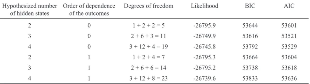
We fitted independent or first-order dependent out-comes and up to four latent states. Table 1 summarizes the

results. BIC and AIC (see Schwarz, 1978 and Sakamotoet

al., 1986) pointed out a three-state independent outcome

model as the one providing the best fit.

Figure 2 shows the smoothed estimates of localC + G

composition based on a three-state independent outcome model . The local composition was estimated as:

$

πt t,1 t,1 t,1

n

i 1

P(y s )P(s y )

=

=

∑

In (19) yt,1implies we are dealing with local

propor-tion ofC + G -there are only two outcomes: 1 (for C or G)

or 2 (for A or T).

In Figure 2 we notice that there are four regions. The

first and the last one present comparableC + Gsmoothed

proportions.

The second region is the largest and presents the larg-estC + Gconcentration. Region three is narrow and spiked. Approximately first region ranges from base 1 to 7,000, the second region goes up to base 21,000, and the third goes from base 22,000 to 24,000. Regions one and two are in very good agreement with our data description, matching

energy metabolism and RNA processing genes. Region three incorporates, functionally speaking, very heteroge-neous data, so it is not possible to characterize it in those

Table 1- Summary statistics used for selecting the best HMM model for theXylelladataset.

Hypothesized number of hidden states

Order of dependence of the outcomes

Degrees of freedom Likelihood BIC AIC

2 0 1 + 2 + 2 = 5 -26795.9 53644 53601 3 0 2 + 6 + 3 = 11 -26749.9 53616 53521 4 0 3 + 12 + 4 = 19 -26745.8 53792 53529 2 1 1 + 2 + 4 = 7 -26795.3 53664 53604 3 1 2 + 6 + 6 = 14 -26795.2 53738 53618 4 1 3 + 12 + 8 = 23 -26739.6 53833 53636

Figure 1- Plot of the local proportions of A+T based on a four-state model

terms. Region four is well defined with a regular low

ex-pression ofC + G. It does not contradict the data

descrip-tion in the sense that approximately from bases 26,000 to 32,000 the smoothed proportions show homogeneity which

matches the location ofmacromolecule metabolismgenes.

These results confirm that hidden Markov models are use-ful tools to reveal homogeneous regions of DNA data.

We notice that there are non negligible differences in scale of the maps obtained for the studied organisms. We can observe that the homogeneous regions are separated more clearly in the case of the phage. This might be due to

the weaker kind of dependencies in theXylella data we

worked with compared to the phage data. Despite the fact that the best model was found to be a three state one, model selection procedures did not support first order

dependen-cies amongXylella outcomes in contrast with the phage

outcomes. Therefore, it is reasonable that the phage map presents a better discrimination of homogeneous regions

than theXylellamap.

Finally, even though we could tell the major function

of the genes included in theXylelladataset we used by

in-specting the chromossome map (website http://aeg.lbi.ic. unicamp.br/xf/), this is no longer feasible when dealing

with the whole genome of theXylellagenome. Thus,

com-putational methods are needed to extract and summarize major underlying features that help the analyst to under-stand DNA structure and function. Hidden Markov models seem to be a good option.

Discussion

Hidden Markov models are useful for describing and revealing some special features of temporal biological se-ries. The main advantage over the regular Markov models is the possibility that HMMs have of accounting for hetero-geneity that may be present in the data. As a result, more sensible models and better data descriptions might be avail-able to the analyst.

In this work we applied HMM methods to a

subsequence of theXylella fastidiosagenome. In order to

describe possible variations in the expression ofC + G,we

worked with theC + Gsequence data instead of with the

original DNA sequence. The HMM that better describes the data was able to correctly discriminate regions in the data corresponding to distinct biological functions. In the future, this kind of model may be used in the study of larger

subse-quences or even the wholeXylellagenome.

There are other already known uses of HMM in

com-putational biology. Those may be tried on theXylelladata.

For example, HMMs are used for obtaining multiple aligned sequences and also for gene detection.

According to Hugley and Krogh (1996), HMM are a highly effective means of modeling a family of unaligned sequences or a common motif within a set of unaligned se-quences. HMMs are particularly useful in the study of pro-tein molecules since they make possible the automatic discrimination of evolutionarily close proteins. Proteins are built from an alphabet of twenty smaller molecules known as amino acids. According to http://www.cse.ucsc.edu/re-search/compbio/ismb99.handouts/KK185FP.html, when a cell reproduces, a protein inside the cell is most of the time exactly duplicated in the daughter cell. However, over long periods of time, errors occur in the copy process. When this happens, a protein in the daughter cell is slightly different from its counterpart in the parent. The three most common errors are “substitution” of an amino acid in a given posi-tion, “insertion” of one or more new amino acids, and “de-letion” of one or more amino acids. As a result of these errors, proteins which share a common ancestor are not ex-actly alike. However, they inherit many similarities in pri-mary structure from their ancestor. This is known as “conservation” of primary structure in a protein family. In an HMM for multiple alignment the states are S (substitu-tion), I (inser(substitu-tion), D (deletion) and M (matching of amino

acids). According to Kroghet al. (1994), an HMM used for

multiple alignment identifies a set of positions that de-scribes the conserved primary structure in the sequences

from a given family of proteins,i.e., the model identifies

the core elements of homologous proteins. In the case of the

Xylella it may be important to know how evolutionarily close is this organism to another, since similar methods used in the combat of the latter could be tried.

HMMs are also a very useful tool in gene prediction. According to Stormo (2000), the states correspond to exons, introns, and any other class of sequences desired (such as 5’ and 3’ UTRs, promoters regions, intergenic re-gions, repetitive DNA, etc). These genetic entities signal the points in the DNA where a new gene starts or ends. The probability of changing from an intron to an exon depends on the local sequence such that it is high only at plausible splice junctions. Stormo (2000) explains that the “hidden” in these HMMs denotes that fact that we see only the DNA sequence directly, and the state that generated the sequence

Figure 2- Plot of the local proportions of C+G based on a three-state

(exon, intron, etc) is not visible. These methods are impor-tant because genes can be located using computational biol-ogy tools.

Acknowledgments

We would like to thank the anonymous referees for valuable comments and suggestions on this study.

References

Agresti A (1990) Categorical Data Analysis. 1st ed. John Wiley & Sons, New York.

Anderson TW and Goodman LA (1957) Statistical Inference About Markov Chains. Annals Math Statist 28:89-110. Arnold J, Cuticchia AJ, Newsome DA, Jennings III, WW and

Ivarie R (1988) Mono-through hexanucleotide composition of the sense strand of yeast DNA: A Markov chain analysis. Nucleic Acids Res 16:7145-7158.

Avery PJ (1987) The analysis of Intron data and their use in the detection of short signals. Journal of Molecular Evolution 26:335-340.

Avery PJ and Henderson DA (1999) Fitting Markov chain models to discrete state series such as DNA sequences. Applied Sta-tistics 48, Part 1:53-61.

Bernardi G and Bernardi G (1986) Compositional constraints and genome evolution. J Mol Evol 24:1-11.

Bishop YMM, Fienberg SE, Holland PW, Mosteller F and Light R (1975) Discrete Multivariate Analysis: Theory and Practice. 1st ed. The MIT Press, Massachusetts.

Boys RJ, Henderson DA and Wilkinson DJ (2000) Detecting ho-mogeneous segments in DNA sequences by using hidden Markov models. Applied Statistics 49 Part 2:269:285. Chen J, Jarret RL, Qin X, Hartung JS, Banks D, Chang CJ and

Hopkins DL (2000) 16S rDNA sequence analysis ofXylella fastidiosa strains. Systematic and Applied Microbiology 23(3):349-354.

Churchill GA (1989) Stochastic models for heterogenous DNA sequences. Bulletin of Mathematical Biology 51(1):79-94. Guilhabert MR, Hoffman LM, Mills DA and Kirkpatrick BC

(2001) Transposon mutagenesis of Xylella fastidiosa by electroporation of Tn5 synaptic complexes. Molecular Plant-Microbe Interactions 14(6):701-706.

Hughey R and Krogh A (1996) Hidden Markov models for se-quence analysis: extensions and analysis of the basic method. CABIOS 12(2):95-107.

Krogh A, Brown M, Mian S, Sjolander K and Haussler D (1994) Hidden Markov models in computational biology. Recent Methods for RNA Modeling Using Stochastic Context-Free Grammars. CPM: 289-306

Lambais MR, Goldman MHS, Camargo LEA and Goldman GH (2000) A genomic approach to the understanding ofXylella fastidiosapathogenicity. Current Opinion in Microbiology 3(5):459-462.

McCullagh P and Nelder JA (1989) Generalized Linear Models. 2nd ed. Chapman & Hall, London.

Mehta A, Leite RP and Rosato YB (2001) Assessment of the ge-netic diversity ofXylella fastidiosaisolated from citrus in Brazil by PCR-RFLP of the 16S rDNA and 16S-23S intergenic spacer and rep-PCR fingerprinting. Antonie Van Leeuwenhoek International Journal of General and Molecu-lar Microbiology 79(1):53-59.

Qin XT, Miranda VS, Machado MA, Lemos EGM and Hartung JS (2000) An evaluation of the genetic diversity of Xylella fastidiosaisolated from diseased citrus and coffee in Sao Paulo, Brazil. Phytopathology 91(6):599-605.

Raftery A (1986) Choosing Models for Cross-classifications, Amer Sociol Rev 51:145-146.

Raftery A (1995) Bayesian Model Selection in Social Research (with Discussion). University of Washington Demography Center Working Paper . 94-12. A revised version appeared in Sociological Methodology 1995, pp 111-196.

Raftery A and Tavare S (1994) Estimation and Modelling Re-peated Patterns in High Order Markov Chains with the Mix-ture Transition Distribution Model, Applied Statistics 43(1):179-199.

Sakamoto Y, Ishiguro M and Kitagawa G (1986) Akaike Informa-tion Criterion Statistics, D. Reidel Publishing Company. Schwarz G (1978) Estimating the dimension of a model. Annals

of Statistics 6:461-464.

Skalka A, Burgi E and Hershey AD (1968) Segmental distribution of nucleotide sequence of Bacteriophage lambda DNA. J Mol Biol 162:729-773.

Stormo GD (2000) Gene-finding approaches for eukaryots. Ge-nome Research 10:394-397.

Tavaré S and Giddings BW (1989) Some statistical aspects of the primary structure of nucleotide sequences. In: Waterman MS (ed) Mathematical Methods for DNA Sequences. CRC Press, Boca Raton, FL, pp 117-132.

Weir BS (1996) Genetic Data Analysis II, 1st. ed., Sinauer Asso-ciates, Inc., Sunderland.