RESEARCH ARTICLE
Fast Bayesian Inference of Copy Number
Variants using Hidden Markov Models with
Wavelet Compression
John Wiedenhoeft, Eric Brugel, Alexander Schliep*
Department of Computer Science, Rutgers University, Piscataway, New Jersey, United States of America *alexander@schlieplab.org
Abstract
By integrating Haar wavelets with Hidden Markov Models, we achieve drastically reduced running times for Bayesian inference using Forward-Backward Gibbs sampling. We show that this improves detection of genomic copy number variants (CNV) in array CGH experi-ments compared to the state-of-the-art, including standard Gibbs sampling. The method concentrates computational effort on chromosomal segments which are difficult to call, by dynamically and adaptively recomputing consecutive blocks of observations likely to share a copy number. This makes routine diagnostic use and re-analysis of legacy data collec-tions feasible; to this end, we also propose an effective automatic prior. An open source software implementation of our method is available athttp://schlieplab.org/Software/ HaMMLET/(DOI:10.5281/zenodo.46262). This paper was selected for oral presentation at RECOMB 2016, and an abstract is published in the conference proceedings.
This is aPLOS Computational BiologySoftware paper.
Introduction
The human genome shows remarkable plasticity, leading to significant copy number variations (CNV) within the human population [1]. They contribute to differences in phenotype [2–4], ranging from benign variation over disease susceptibility to inherited and somatic diseases [5], including neuropsychiatric disorders [6–8] and cancer [9,10]. Separating common from rare variants is important in the study of genetic diseases [5,11,12], and while the experimental platforms have matured, interpretation and assessment of pathogenic significance remains a challenge [13].
Computationally, CNV detection is a segmentation problem, in which consecutive stretches of the genome are to be labeled by their copy number; following the conventions typically employed in CNV method papers, e.g. [14–17], we use this term rather abstractly to denote a11111
OPEN ACCESS
Citation:Wiedenhoeft J, Brugel E, Schliep A (2016) Fast Bayesian Inference of Copy Number Variants using Hidden Markov Models with Wavelet Compression. PLoS Comput Biol 12(5): e1004871. doi:10.1371/journal.pcbi.1004871
Editor:Paul P Gardner, University of Canterbury, NEW ZEALAND
Received:November 26, 2015 Accepted:March 14, 2016 Published:May 13, 2016
Copyright:© 2016 Wiedenhoeft et al. This is an open access article distributed under the terms of the
Creative Commons Attribution License, which permits unrestricted use, distribution, and reproduction in any medium, provided the original author and source are credited.
segments of equal mean value, not actual ploidy, though for homogeneous samples the latter can be easily assigned. Along with a variety of other methods [14–16,18–41], Hidden Markov Models (HMM) [42] play a central role [17,43–52], as they directly model the separate layers of observed measurements, such as log-ratios in array comparative genomic hybridization (aCGH), and their corresponding latent copy number (CN) states, as well as the underlying lin-ear structure of segments.
As statistical models, they depend on a large number of parameters, which have to be either provideda prioriby the user or inferred from the data. Classic frequentist maximum likelihood (ML) techniques like Baum-Welch [53,54] are not guaranteed to be globally optimal, i. e. they can converge to the wrong parameter values, which can limit the accuracy of the segmentation. Furthermore, the Viterbi algorithm [55] only yields a single maximum a posteriori (MAP) seg-mentation given a parameter estimate [56]. Failure to consider the full set of possible parame-ters precludes alternative interpretations of the data, and makes it very difficult to derivep -values or confidence intervals. Furthermore, these frequentist techniques have come under increased scrutiny in the scientific community.
Bayesian inference techniques for HMMs, in particular Forward-Backward Gibbs sampling [57,58], provide an alternative for CNV detection as well [59–61]. Most importantly, they yield a complete probability distribution of copy numbers for each observation. As they are sampling-based, they are computationally expensive, which is problematic especially for high-resolution data. Though they are guaranteed to converge to the correct values under very mild assumptions, they tend to do so slowly, which can lead to oversegmentation and mislabeling if the sampler is stopped prematurely.
Another issue in practice is the requirement to specify hyperparameters for the prior distri-butions. Despite the theoretical advantage of making the inductive bias more explicit, this can be a major source of annoyance for the user. It is also hard to justify any choice of hyperpara-meters when insufficient domain knowledge is available.
Recent work of our group [62] has focused on accelerating Forward-Backward Gibbs sam-pling through the introduction of compressed HMMs and approximate samsam-pling. For the first time, Bayesian inference could be performed at running times on par with classic maximum likelihood approaches. It was based on a greedy spatial clustering heuristic, which yielded a static compression of the data into blocks, and block-wise sampling. Despite its success, several important issues remain to be addressed. The blocks are fixed throughout the sampling and impose a structure that turns out to be too rigid in the presence of variances differing between CN states. The clustering heuristic relies on empirically derived parameters not supported by a theoretical analysis, which can lead to suboptimal clustering or overfitting. Also, the method cannot easily be generalized for multivariate data. Lastly, the implementation was primarily aimed at comparative analysis between the frequentist and Bayesian approach, as opposed to overall speed.
To address these issues and make Bayesian CNV inference feasible even on a laptop, we pro-pose the combination of HMMs with another popular signal processing technology: Haar wavelets have previously been used in CNV detection [63], mostly as a preprocessing tool for statistical downstream applications [28–32] or simply as a visual aid in GUI applications [21,
64]. A combination of smoothing and segmentation has been suggested as likely to improve results [65], and here we show that this is indeed the case. Wavelets provide a theoretical foun-dation for a better, dynamic compression scheme for faster convergence and accelerated Bayes-ian sampling (Fig 1). We improve simultaneously upon the typically conflicting goals of accuracy and speed, because the wavelets allow summary treatment of“easy”CN calls in seg-ments and focus computational effort on the“difficult”CN calls, dynamically and adaptively. This is in contrast to other computationally efficient tools, which often simplify the statistical our supplemental data has been deposited for open
access athttps://zenodo.org/record/46263. Funding:This work was funded by: EB: National Science Foundation "Research Experience for Undergraduates", award 1263082,http://www.nsf. gov/awardsearch/showAward?AWD_ID=1263082; AS: National Institute of Health: "Meaningful Data Compression and Reduction of High-Throughput Sequencing Data", award 1 U01 CA198952-01,
https://datascience.nih.gov/bd2k/funded-programs/ software. The funders had no role in study design, data collection and analysis, decision to publish, or preparation of the manuscript.
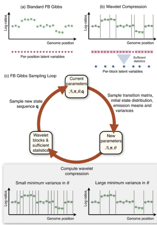
Fig 1. Overview of HaMMLET.Instead of individual computations per observation (panel a), Forward-Backward Gibbs Sampling is performed on a compressed version of the data, using sufficient statistics for block-wise computations (panel b) to accelerate inference in Bayesian Hidden Markov Models. During the sampling (panel c) parameters and copy number sequences are sampled iteratively. During each iteration, the sampled emission variances determine which coefficients of the data’s Haar wavelet transform are dynamically set to zero. This controls potential break points at finer or
model or use heuristics. The required data structure can be efficiently computed, incurs mini-mal overhead, and has a straightforward generalization for multivariate data. We further show how the wavelet transform yields a natural way to set hyperparameters automatically, with little input from the user.
We implemented our method in a highly optimized end-user software, called HaMMLET. Aside from achieving an acceleration of up to two orders of magnitude, it exhibits significantly improved convergence behavior, has excellent precision and recall, and provides Bayesian inference within seconds even for large data sets. The accuracy and speed of HaMMLET also makes it an excellent choice for routine diagnostic use and large-scale re-analysis of legacy data. Notice that while we focus on aCGH in this paper as the most straightforward biological example of univariate Gaussian data, the method we present is a general approach to Bayesian HMM inference as long as the emission distributions come from the exponential family, imply-ing that conjugate priors exist and the dimension of its sufficient statistics remain bounded with increasing sample size. It can thus be readily generalized and adapted to read-depth data, SNP arrays, and multi-sample applications.
Results
Simulated aCGH data
A previous survey [65] of eleven CNV calling methods for aCGH has established that segmenta-tion-focused methods such as DNAcopy [14,36], an implementation of circular binary segmen-tation (CBS), as well as CGHseg [37] perform consistently well. DNAcopy performs a number of t-tests to detect break-point candidates. The result is typically over-segmented and requires a merging step in post-processing, especially to reduce the number of segment means. To this end MergeLevels was introduced by [66]. They compare the combination DNAcopy+MergeLevels to their own HMM implementation [17] as well as GLAD (Gain and Loss Analysis of DNA) [27], showing its superior performance over both methods. This established DNAcopy+MergeLevels as thede factostandard in CNV detection, despite the comparatively long running time.
The paper also includes aCGH simulations deemed to be reasonably realistic by the commu-nity. DNAcopy was used to segment 145 unpublished samples of breast cancer data, and subse-quently labeled as copy numbers 0 to 5 by sorting them into bins with boundaries (−1,−0.4,
−0.2, 0.2, 0.4, 0.6,1), based on the sample mean in each segment (the last bin appears to not
be used). Empirical length distributions were derived, from which the sizes of CN aberrations are drawn. The data itself is modeled to include Gaussian noise, which has been established as sufficient for aCGH data [67]. Means were generated such as to mimic random tumor cell pro-portions, and random variances were chosen to simulate experimenter bias often observed in real data; this emphasizes the importance of having automatic priors available when using Bayesian methods, as the means and variances might be unknowna priori. The data comprises three sets of simulations:“breakpoint detection and merging”(BD&M),“spatial resolution study”(SRS), and“testing”(T) (see their paper for details). We used the MergeLevels imple-mentation as provided on their website. It should be noted that the superiority of DNAcopy+-MergeLevels was established using a simulation based upon segmentation results of DNAcopy itself.
CBS [15]; note that other authors such as [35] compare against a quadratic-time version of CBS [14], which is significantly slower. For HaMMLET, we use a 5-state model with automatic hyperparametersPðs2
0:01Þ ¼0:9(see sectionAutomatic priors), and all Dirichlet
hyper-parameters set to 1.
Following [62], we report F-measures (F1scores) for binary classification into normal and
aberrant segments (Fig 2), using the usual definition ofF¼2pr
pþrbeing the harmonic mean of
precisionp¼ TP
TPþFPand recallr¼ TP
TPþFN, where TP, FP, TN and FN denote true/false positives/ negatives, respectively. On datasets T and BD&M, both methods have similar medians, but HaMMLET has a much better interquartile range (IQR) and range, about half of CBS’s. On the spatial resolution data set (SRS), HaMMLET performs much better on very small aberrations. This might seem somewhat surprising, as short segments could easily get lost under compres-sion. However, Laiet al.[65] have noted that smoothing-based methods such as quantile smoothing (quantreg) [23], lowess [24], and wavelet smoothing [29] perform particularly well in the presence of high noise and small CN aberrations, suggesting that“an optimal combina-tion of the smoothing step and the segmentacombina-tion step may result in improved performance”. Our wavelet-based compression inherits those properties. For CNVs of sizes between 5 and 10, CBS and HaMMLET have similar ranges, with CBS being skewed towards better values; CBS has a slightly higher median for 10–20, with IQR and range being about the same. However, while HaMMLET’s F-measure consistently approaches 1 for larger aberrations, CBS does not appear to significantly improve after size 10. The plots for all individual samples can be found in Web Supplement S1–S3, which can be viewed online athttp://schlieplab.org/Supplements/
HaMMLET/, or downloaded fromhttps://zenodo.org/record/46263(DOI:10.5281/zenodo.
46263).
High-density CGH array
In this section, we demonstrate HaMMLET’s performance on biological data. Due to the lack of a gold standard for high-resolution platforms, we assess the CNV calls qualitatively. We use raw aCGH data (GEO:GSE23949) [68] of genomic DNA from breast cancer cell line BT-474 (invasive ductal carcinoma, GEO:GSM590105), on an Agilent-021529 Human CGH Whole Genome Microarray 1x1M platform (GEO:GPL8736). We excluded gonosomes, mitochondrial and random chromosomes from the data, leaving 966,432 probes in total.
HaMMLET allows for using automatic emission priors (see sectionAutomatic priors) by specifying a noise variance, and a probability to sample a variance not exceeding this value. We compare HaMMLET’s performance against CBS, using a 20-state model with automatic priors,
Pðs2
0:1Þ ¼0:8, 10 prior self-transitions and 1 for all other hyperparameters. CBS took over
2 h 9 m to process the entire array, whereas HaMMLET took 27.1 s for 100 iterations, a speedup of 288. The compression ratio (see section Effects of wavelet compression on speed and conver-gence) was 220.3. CBS yielded a massive over-segmentation into 1,548 different copy number levels; cf. Web Supplement S4 athttps://zenodo.org/record/46263. As the data is derived from a relatively homogeneous cell line as opposed to a biopsy, we do not expect the presence of subclo-nal populations to be a contributing factor [69,70]. Instead, measurements on aCGH are known to be spatially correlated, resulting in a wave pattern which has to be removed in a pre-processing step; notice that the internal compression mechanism of HaMMLET is derived from a spatially adaptive regression method, so smoothing is inherent to our method. CBS performs such a smoothing, yet an unrealistically large number of different levels remains, likely due to residuals of said wave pattern. Furthermore, repeated runs of CBS yielded different numbers of levels, suggesting that indeed the merging was incomplete. This can cause considerable prob-lems downstream, as many methods operate on labeled data. A common approach is to
consider a small number of classes, typically 3 to 4, and associate them semantically with CN labels likeloss,neutral,gain, andamplification, e.g. [27,59,61,67,71–75]. In inference models that contain latent categorical state variables, like HMM, such an association is readily achieved by sorting classes according to their means. In contrast, methods like CBS typically yield a large, often unbounded number of classes, and reducing it is the declared purpose of merging algo-rithms, see [66]. Consider, for instance, CGHregions [74], which uses a 3-label matrix to define regions of shared CNV events across multiple samples by requiring a maximumL1distance of
label signatures between all probes in that region. If the domain of class labels was unrestricted and potentially different in size for each sample, such a measure would not be meaningful, since thei-th out ofnclasses cannot be readily identified with thei-th out ofmclasses forn6¼m, hence no two classes can be said to represent the same CN label. Similar arguments hold true for clustering based on Hamming distance [72] or ordinal similarity measures [71]. Further-more, even CGHregions’s optimized computation of medoids takes several minutes to compute. As the time depends multiplicatively on the number of labels, increasing it by three orders of magnitude would increase downstream running times to many hours.
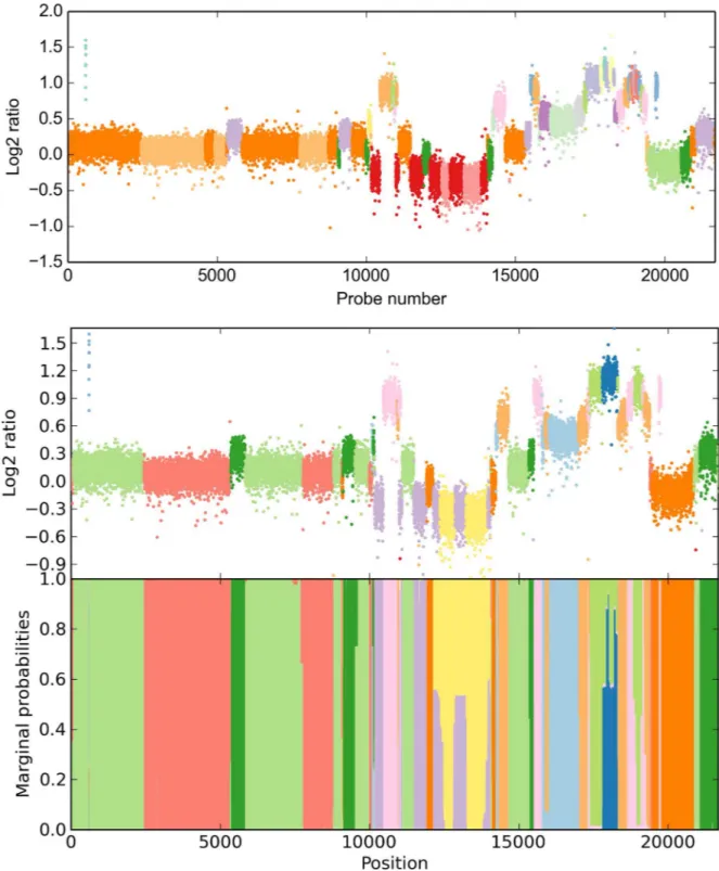
For a more comprehensive analysis, we restricted our evaluation to chromosome 20 (21,687 probes), which we assessed to be the most complicated to infer, as it appears to have the highest number of different CN states and breakpoints. CBS yields a 19-state result after 15.78 s (Fig 3, top). We have then used a 19-state model with automated priors (Pðs2
0:04Þ ¼0:9Þ, 10
prior self-transitions, all other Dirichlet parameters set to 1) to reproduce this result. Using noise control (seeMethods), our method took 1.61 s for 600 iterations. The solution we obtained is consistent with CBS (Fig 3, middle and bottom). However, only 11 states were part of thefinal solution, i. e. 8 states yielded no significant likelihood above that of other states. We
Fig 2. F-measures of CBS (light) and HaMMLET (dark) for calling aberrant copy numbers on simulated aCGH data [66].Boxes represent the interquartile range (IQR = Q3−Q1), with a horizontal line showing the median (Q2), whiskers representing the range (3
2IQRbeyond Q1 and Q3), and the bullet representing the mean. HaMMLET has the same or better F-measures in most cases, and on the SRS simulation converges to 1 for larger segments, whereas CBS plateaus for aberrations greater than 10.
Fig 3. Copy number inference for chromosome 20 in invasive ductal carcinoma (21,687 probes).CBS creates a 19-state solution (top), however, a compressed 19-state HMM only supports an 11-state solution (bottom), suggesting insufficient level merging in CBS.
doi:10.1371/journal.pcbi.1004871.g003
observe superfluous states being ignored in our simulations as well. In light of the results on the entire array, we suggest that the segmentation by DNAcopy has not sufficiently been merged by MergeLevels. Most strikingly, HaMMLET does not show any marginal support for a segment called by CBS around probe number 4,500. We have confirmed that this is not due to data compression, as the segment is broken up into multiple blocks in each iteration (cf. Web Supplement S5 athttps://zenodo.org/record/46263). On the other hand, two much smaller segments called by CBS in the 17,000–20,000 range do have marginal support of about 40% in HaMMLET, suggesting that the lack of support for the larger segment is correct. It should be noted that inference differs between the entire array and chromosome 20 in both methods, since long-range effects have higher impact in larger data.
We also demonstrate another feature of HaMMLET callednoise control. While Gaussian emissions have been deemed a sufficiently accurate noise model for aCGH [67], microarray data is prone to outliers, for example due to damages on the chip. While it is possible to model outliers directly [60], the characteristics of the wavelet transform allow us to largely suppress them during the construction of our data structure (seeMethods). Notice that due to noise control most outliers are correctly labeled according to the segment they occur in, while the short gain segment close to the beginning is called correctly.
Effects of wavelet compression on speed and convergence
The speedup gained by compression depends on how well the data can be compressed. Poor compression is expected when the means are not well separated, or short segments have small variance, which necessitates the creation of smaller blocks for the rest of the data to expose potential low-variance segments to the sampler. On the other hand, data must not be over-compressed to avoid merging small aberrations with normal segments, which would decrease the F-measure. Due to the dynamic changes to the block structure, we measure the level of compression as the average compression ratio, defined as the product of the number of data pointsTand the number of iterationsN, divided by the total number of blocks in all iterations. As usual a compression ratio of one indicates no compression.
To evaluate the impact of dynamic wavelet compression on speed and convergence proper-ties of an HMM, we created 129,600 different data sets withT= 32,768 many probes. In each data set, we randomly distributed 1 to 6 gains of a total length of {100, 250, 500, 750, 1000} uni-formly among the data, and do the same for losses. Mean combinations (μloss,μneutral,μgain)
were chosen from log2 1
2;log21;log2 3 2
, (−1, 0, 1), (−2, 0, 2), and (−10, 0, 10), and variances
ðs2 loss;s
2 neutral;s
2
gainÞfrom (0.05, 0.05, 0.05), (0.5, 0.1, 0.9), (0.3, 0.2, 0.1), (0.2, 0.1, 0.3), (0.1, 0.3, 0.2), and (0.1, 0.1, 0.1). These values have been selected to yield a wide range of easy and hard cases, both well separated, low-variance data with large aberrant segments as well as cases in which small aberrations overlap significantly with the tail samples of high-variance neutral seg-ments. Consequently, compression ratios range from*1 to*2, 100. We use automatic priors
Pðs2
0:2Þ ¼0:9, self-transition priorsαii2{10, 100, 1000}, non-self transition priorsαij= 1,
and initial state priorsα2{1,10}. Using all possible combinations of the above yields 129,600
different simulated data sets, a total of 4.2 billion values.
uncompressed version took over 3 weeks and 5 days. All running times reported are CPU time measured on a single core of a AMD Opteron 6174 Processor, clocked at 2.2 GHz.
We evaluate the convergence of the F-measure of compressed and uncompressed inference for each simulation. Since we are dealing with multi-class classification, we use the micro- and macro-averaged F-measures (Fmi,Fma) proposed by [76]:
Fmi¼ 2pr
pþr with p¼
PM
i¼1TPi
PM
i¼1ðTPiþFPiÞ
; r¼
PM
i¼1TPi
PM
i¼1ðTPiþFNiÞ and
Fma¼
PM
i¼1Fi
M with pi¼ TPi TPiþFPi
; ri¼ TPi
TPiþFNi
; Fi ¼ 2p
iri piþri:
Here, TPidenotes a true positive call for thei-th out ofMstates,πandρdenote precision and recall. These F-measures tend to be dominated by the classifier’s performance on common and rare categories, respectively. Since all state labels are sampled from the same prior and hence their relative order is random, we used the label permutation which yielded the highest sum of micro- and macro-averaged F-measures. The simulation results are included in Web Supple-ment S6 athttps://zenodo.org/record/46263.
InFig 5, we show that the compressed version of the Gibbs sampler converges almost
instantly, whereas the uncompressed version converges much slower, with about 5% of the cases failing to yield an F-measure>0.6 within 1,000 iterations. Wavelet compression is likely to yield reasonably large blocks for the majority class early on, which leads to a strong posterior estimate of its parameters and self-transition probabilities. As expected,Fmaare generally worse, since any
misclassification in a rare class has a larger impact. Especially in the uncompressed version, we
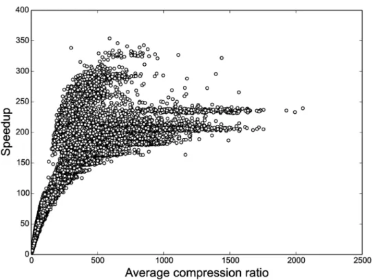
Fig 4. HaMMLET’s speedup as a function of the average compression during sampling.As expected, higher compression leads to greater speedup. The non-linear characteristic is due to the fact that some overhead is incurred by the dynamic compression, as well as parts of the implementation that do not depend on the compression, such as tallying marginal counts.
doi:10.1371/journal.pcbi.1004871.g004
observe thatFmatends to plateau untilFmiapproaches 1.0. Since any misclassification in the
majority (neutral) class adds false positives to the minority classes, this effect is expected. It implies that correct labeling of the majority class is a necessary condition for correct labeling of minority classes, in other words, correct identification of the rare, interesting segments requires the sampler to properly converge, which is much harder to achieve without compression. It should be noted that running compressed HaMMLET for 1,000 iterations is unnecessary on the simulated data, as in all cases it converges between 25 and 50 iterations. Thus, for all practical purposes, further speedup by a factor of 40–80 can be achieved by reducing the number of itera-tions, which yields convergence up to 3 orders of magnitude faster than standard FBG.
Coriell, ATCC and breast carcinoma
The data provided by [77] includes 15 aCGH samples for the Coriell cell line. At about 2,000 probes, the data is small compared to modern high-density arrays. Nevertheless, these data sets
Fig 5. F-measures for simulation results.The median value (black) and quantile ranges (in 5% steps) of the micro- (top) and macro-averaged (bottom) F-measures (Fmi,Fma) for uncompressed (left) and compressed (right) FBG inference, on the same 129,600 simulated data sets, using automatic priors. The x-axis represents the number of iterations alone, and does not reflect the additional speedup obtained through compression. Notice that the compressed HMM converges no later than 50 iterations (inset figures, right).
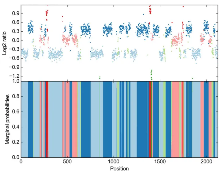
have become a common standard to evaluate CNV calling methods, as they contain few and simple aberrations. The data also contains 6 ATCC cell lines as well as 4 breast carcinoma, all of which are substantially more complicated, and typically not used in software evaluations. In
Fig 6, we demonstrate our ability to infer the correct segments on the most complex example, a
T47D breast ductal carcinoma sample of a 54 year old female. We used 6-state automatic priors withPðs2
0:1Þ ¼0:85, and all Dirichlet hyperparameters set to 1. On a standard laptop,
HaMMLET took 0.09 seconds for 1,000 iterations; running times for the other samples were similar. Our results for all 25 data sets have been included in Web Supplement S7 athttps://
zenodo.org/record/46263.
Discussion
In the analysis of biological data, there are usually conflicting objectives at play which need to be balanced: the required accuracy of the analysis, ease of use—using the software, setting soft-ware and method parameters—and often the speed of a method. Bayesian methods have obtained a reputation of requiring enormous computational effort and being difficult to use, for the expert knowledge required for choosing prior distributions. It has also been recognized
Fig 6. HaMMLET’s inference of copy-number segments on T47D breast ductal carcinoma.Notice that the data is much more complex than the simple structure of a diploid majority class with some small aberrations typically observed for Coriell data. doi:10.1371/journal.pcbi.1004871.g006
[60,62,78] that they are very powerful and accurate, leading to improved, high-quality results and providing, in the form of posterior distributions, an accurate measure of uncertainty in results. Nevertheless, it is not surprising that a hundred times larger effort in computation alone prevented wide-spread use.
Inferring Copy Number Variants (CNV) is a quite special problem, as experts can identify CN changes visually, at least on very good data and for large, drastic CN changes (e. g., long segments lost on both chromosomal copies). With lesser quality data, smaller CN differences and in the analysis of cohorts the need for objective, highly accurate, and automated methods is evident.
The core idea for our method expands on our prior work [62] and affirms a conjecture by Laiet al.[65] that a combination of smoothing and segmentation will likely improve results. One ingredient of our method are Haar wavelets, which have previously been used for pre-pro-cessing and visualization [21,64]. In a sense, they quantify and identify regions of high varia-tion, and allow to summarize the data at various levels of resoluvaria-tion, somewhat similar to how an expert would perform a visual analysis. We combine, for the first time, wavelets with a full Bayesian HMM by dynamically and adaptively infering blocks of subsequent observations from our wavelet data structure. The HMM operates on blocks instead of individual observa-tions, which leads to great saving in running times, up to 350-fold compared to the standard FB-Gibbs sampler, and up to 288 times faster than CBS. Much more importantly, operating on the blocks greatly improves convergence of the sampler, leading to higher accuracy for a much smaller number of sampling iterations. Thus, the combination of wavelets and HMM realizes a simultaneous improvement on accuracy and on speed; typically one can have one or the other. An intuitive explanation as to why this works is that the blocks derived from the wavelet struc-ture allow efficient, summary treatment of those“easy”to call segments given the current sam-ple of HMM parameters and identifies“hard”to call CN segment which need the full
computational effort from FB-Gibbs. Note that it is absolutely crucial that the block structure depends on the parameters sampled for the HMM and will change drastically over the run time. This is in contrast to our prior work [62], which used static blocks and saw no improve-ments to accuracy and convergence speed. The data structures and linear-time algorithms we introduce here provide the efficient means for recomputing these blocks at every cycle of the sampling, cf.Fig 1. Compared to our prior work, we observe a speed-up of up to 3,000 due to the greatly improved convergence,O(T) vs.O(TlogT) clustering, improved numerics and, lastly, a C++ instead of a Python implementation.
We performed an extensive comparison with the state-of-the-art as identified by several review and benchmark publications and with the standard FB-Gibbs sampler on a wide range of biological data sets and 129,600 simulated data sets, which were produced by a simulation process not based on HMM to make it a harder problem for our method. All comparisons demonstrated favorable results for our method when measuring accuracy at a very noticeable acceleration compared to the state-of-the-art. It must be stressed that these results were obtained with a statistically sophisticated model for CNV calls and without cutting algorithmic corners, but rather an effective allocation of computational effort.
from non-automatic, expert-selected priors, but refrained from using them for the evaluation, as they might be perceived as unfair to other methods.
In summary, our method is as easy to use as other, statistically less sophisticated tools, more accurate and much more computationally efficient. We believe this makes it an excellent choice both for routine use in clinical settings and principled re-analysis of large cohorts, where the added accuracy and the much improved information about uncertainty in copy number calls from posterior marginal distributions will likely yield improved insights into CNV as a source of genetic variation and its relationship to disease.
Methods
We will briefly review Forward-Backward Gibbs sampling (FBG) for Bayesian Hidden Markov Models, and its acceleration through compression of the data into blocks. By first considering the case of equal emission variances among all states, we show that optimal compression is equivalent to a concept calledselective wavelet reconstruction, following a classic proof in wave-let theory. We then argue thatwavelet coefficient thresholding, a variance-dependent minimax estimator, allows for compression even in the case of unequal emission variances. This allows the compression of the data to be adapted to the prior variance level at each sampling iteration. We then derive a simple data structure to dynamically create blocks with little overhead. While wavelet approaches have been used for aCGH data before [29,33,34,63], our method provides the first combination of wavelets and HMMs.
Bayesian Hidden Markov Models
LetTbe the length of the observation sequence, which is equal to the number of probes. An HMM can be represented as a statistical modelðq;A;y;πjyÞ, with transition matrixA, a
latent state sequenceq= (q0,q1,. . .,qT−1), an observed emission sequencey= (y0,y1,. . .,yT−1),
emission parametersθ, and an initial state distributionπ.
In the usual frequentist approach, the state sequenceqis inferred by first finding a maxi-mum likelihood estimate of the parameters,
ðA
ML;yML;πMLÞ ¼arg max
ðA;y;πÞ
LðA;y;πjyÞ;
using the Baum-Welch algorithm [53,54]. This is only guaranteed to yield local optima, as the likelihood function is not convex. Repeated random reinitializations are used tofind“good” local optima, but there are no guarantees for this method. Then, the most likely state sequence given those parameters,
^
q¼arg max q
PðqjAML;yML;πML;yÞ;
is calculated using the Viterbi algorithm [55]. However, if there are only a few aberrations, that is there is imbalance between classes, the ML parameters tend to overfit the normal state which is likely to yield incorrect segmentation [62]. Furthermore, alternative segmentations given those parameters are also ignored, as are the ones for alternative parameters.
The Bayesian approach is to calculate the distribution of state sequences directly by integrat-ing out the emission and transition variables,
PðqjyÞ ¼
Z
A
Z
y Z
π
Pðq;A;y;πjyÞdπdydA:
techniques, i. e. drawingNsamples,
ðqðiÞ;AðiÞ;yðiÞ;
πðiÞÞ Pðq;A;y;πjyÞ;
and subsequently approximating marginal state probabilities by their frequency in the sample
Pðq
t¼sjyÞ 1
N
XN
i¼1 IðqðiÞ
t ¼sÞ:
Thus, for each positiont, we get a complete probability distribution over the possible states. As the marginals of each variable are explicitly defined by conditioning on the other variables, an HMM lends itself to Gibbs sampling, i. e. repeatedly sampling from the marginals
ðAjq;y;y;πÞ,ðyjq;A;y;πÞ,ðπjA;y;y;qÞ, andðqjA;y;y;πÞ, conditioned on the
previ-ously sampled values. Using Bayes’s formula and several conditional independence relations, the sampling process can be written as
APðAjπ;q;tAÞ / Pðπ;qjAÞPðAjtAÞ;
yPðyjq;y;tyÞ / Pðq;yjyÞPðyjtyÞ;
πPðπjA;q;tπÞ / PðA;qjπÞPðπjtπÞ;and
qPðqjA;y;y;πÞ;
whereτxrepresents hyperparameters to the prior distributionPðxjtxÞ. Typically, each prior will be conjugate, i. e. it will be the same class of distributions as the posterior, which then only depends on updated parametersτ?, e.g.APðAjt?AÞ ¼PðAj
π;q;tAÞ. ThusτπandtAðk;:Þ, the hyperparameters ofπand thek-th row ofA, will be theαiof a Dirichlet distribution, and
τθ= (α,β,ν,μ0) will be the parameters of a Normal-Inverse Gamma distribution.
Notice that the state sequence does not depend on any prior. Though there are several schemes available to sampleq, [58] has argued strongly in favor of Forward-Backward sam-pling [57], which yields Forward-Backward Gibbs sampling (FBG) above. Variations of this have been implemented for segmentation of aCGH data before [60,62,78]. However, since in each iteration a quadratic number of terms has to be calculated at each position to obtain the forward variables, and a state has to be sampled at each position in the backward step, this method is still expensive for large data. Recently, [62] have introducedcompressed FBGby sam-pling over a shorter sequence of sufficient statistics of data segments which are likely to come from the same underlying state. LetB≔ðBwÞ
W
w¼1be a partition ofyintoWblocks. Each block Bwcontainsnwelements. Letyw,kthek-th element inBw. The forward variableαw(j) for this block needs to take into account thenwemissions, the transitions into statej, and thenw−1
self-transitions, which yields
awðjÞ≔Anw 1
jj PðBwjmj;s 2 jÞ
X
nw
i¼1
aw 1ðiÞAij; and
PðBwjm;s2 Þ ¼Y
nw
k¼1
Pðyw;kjm;s2 Þ:
Wavelet theory preliminaries
Here, we review some essential wavelet theory; for details, see [79,80]. Let
cðxÞ
1 0x<1 2
1 1
2x< 1
0 elsewhere
8
> > > > <
> > > > :
be the Haar wavelet [81], andψj,k(x)≔2j/2ψ(2jx−k);jandkare called thescaleandshift
param-eter. Any square-integrable function over the unit interval,f2L2([0,1)), can be approximated using the orthonormal basisfcj;kjj;k2Z; 1j;0k2j 1g, admitting a multiresolu-tion analysis[82, 83]. Essentially, this allows us to express a functionf(x) using scaled and shifted copies of one simple basis functionψ(x) which is spatially localized, i. e. non-zero on only afinite interval inx. The Haar basis is particularly suited for expressing piecewise constant functions.
Finite datay≔(y0,. . .,yT−1) can be treated as an equidistant samplef(x) by scaling the
indi-ces to the unit interval usingxt≔Tt. Leth ≔ log2T. Thenycan be expressed exactly as a linear combination over the Haar wavelet basis above, restricted to the maximum level of sampling resolution (jh−1):
yt¼
X
j;k
dj;kcj;kðxtÞ:
Thewavelet transformd¼Wyis an orthogonal endomorphism, and thus incurs neither redundancy nor loss of information. Surprisingly,dcan be computed in linear time using the pyramid algorithm[82].
Compression via wavelet shrinkage
The Haar wavelet transform has an important property connecting it to block creation: Letd^be a vector obtained by setting elements ofdto zero, theny^¼WTd^
≔W^Tdis calledselective wavelet reconstruction(SW). If all coefficientsdj,kwithψj,k(xt)6¼ψj,k(xt+1) are set to zero for
somet, then^y
t¼^ytþ1, which implies a block structure ony^. Conversely, blocks of size>2 (to account for some pathological cases) can only be created using SW.This general equivalence between SW and compression is central to our method. Note thaty^doesnothave to be computed
explicitly; the block boundaries can be inferred from the position of zero-entries ind^alone. Assume all HMM states had the same emission varianceσ2. Since each state is associated with an emission mean, findingqcan be viewed as a regression or smoothing problem of find-ing an estimateμ^of a piecewise constant functionμwhose range is precisely the set of emission
means, i. e.
μ¼fðxÞ; y¼fðxÞ þ; iidNð0;s2Þ:
Unfortunately, regression methods typically do not limit the number of distinct values recov-ered, and will instead return some estimatey^6¼^μ. However, ify^is piecewise constant and
minimizeskμ y^k, the sample means of each block are close to the true emission means. This
yields high likelihood for their corresponding state and hence a strong posterior distribution, leading to fast convergence. Furthermore, the change points inμmust be close to change points
iny^, since moving block boundaries incurs additional loss, allowing for approximate recovery
of true breakpoints.y^might however induce additional block boundaries that reduce the
com-pression ratio.
In a series of ground-breaking papers, Donoho, Johnstoneet al.[84–88] showed that SW could in theory be used as an almost ideal spatially adaptive regression method. Assuming one could provide an oracleΔ(μ,y) that would know the trueμ, then there exists a method
MSWðy;DÞ ¼ ^ WT
SWusing an optimal subset of wavelet coefficients provided byΔsuch that the quadratic risk ofy^SW≔W^T
SWdis bounded as
kμ y^SWk 2 2¼O
s2 lnT T
:
By definition,MSWwould be the best compression method under the constraints of the Haar
wavelet basis. This bound is generally unattainable, since the oracle cannot be queried. Instead, they have shown that for a methodMWCT(y,λσ) calledwavelet coefficient thresholding, which
sets coefficients to zero whose absolute value is smaller than some thresholdλσ, there exists somel?T ffiffiffiffiffiffiffiffiffiffi
2lnT p
withy^ WCT≔
^ WT
WCTdsuch that
kμ y^WCTk 2
2 ð2lnTþ1Þ kμ y^SWk 2 2þ s2 T :
Thisl?Tis minimax, i. e. the maximum risk incured over all possible data sets is not larger than that of any other threshold, and no better bound can be obtained. It is not easily computed, but for largeT, on the order of tens to hundreds, theuniversal thresholdluT≔pffiffiffiffiffiffiffiffiffiffi2lnTis asymptoti-cally minimax. In other words, for data large enough to warrant compression, universal thresh-olding is the best method to approximateμ, and thus the best wavelet-based compression
scheme for a given noise levelσ2.
Integrating wavelet shrinkage into FBG
This compression method can easily be extended to multiple emission variances. Since we use a thresholding method, decreasing the variance simply subdivides existing blocks. If the threshold is set to the smallest emission variance among all states,y^will approximately
pre-serve the breakpoints around those low-variance segments. Those of high variance are split into blocks of lower sample variance; see [89,90] for an analytic expression. While the vari-ances for the different states are not known, FBG providesa priorisamples in each iteration. We hence propose the following simple adaptation:In each sampling iteration, use the small-est sampled variance parameter to create a new block sequence via wavelet thresholding (Algorithm 1).
Algorithm 1Dynamically adaptive FBG for HMMs
1:procedureHaMMLETðy;tA;ty;tπÞ
2: T |y|
3: l pffiffiffiffiffiffiffiffiffiffiffi2lnT
4: APðAjtAÞ
5: y PðyjtyÞ 6: π PðπjtπÞ 7: fori= 1,. . .,Ndo
8: smin minsifs^
MAD;sijs 2 i 2yg
9: Create block sequenceBfrom thresholdλσmin
10: qPðqjA;B;y;πÞusing Forward-Backward sampling
11: Add count of marginal states forqto result
12: APðAjt?
AÞ ¼PðAjπ;q;tAÞ / Pðπ;qjAÞPðAjtAÞ
13: yPðyjt?
15: end for
16:end procedure
While intuitively easy to understand, provable guarantees for the optimality of this method, specifically the correspondence between the wavelet and the HMM domain remain an open research topic. A potential problem could arise if all sampled variances are too large. In this case, blocks would be under-segmented, yield wrong posterior variances and hide possible state transitions. As a safeguard against over-compression, we use the standard method to estimate the variance of constant noise in shrinkage applications,
^ s2
MAD≔
MADkfdlog2T 1;kg F 1 3
4
!2
as an estimate of the variance in the dominant component, and modify the threshold definition tolminf^s
MAD;si2yg. If the data is not i.i.d.,s^ 2
MADwill systematically underestimate the true variance [28]. In this case, the blocks get smaller than necessary, thus decreasing the compression.
A data structure for dynamic compression
The necessity to recreate a new block sequence in each iteration based on the most recent estimate of the smallest variance parameter creates the challenge of doing so with little computational overhead, specifically without repeatedly computing the inverse wavelet transform or considering allTelements in other ways. We achieve this by creating a simple tree-based data structure.
The pyramid algorithm yieldsdsorted according to (j,k). Again, leth ≔ log2T, andℓ ≔ h−j. We can map the waveletψj,kto a perfect binary tree of heighthsuch that all wavelets for scalejare nodes on levelℓ, nodes within each level are sorted according tok, andℓis increasing
from the leaves to the root (Fig 7).drepresents a breadth-first search (BFS) traversal of that tree, withdj,kbeing the entry at positionb2jc+k. Addingyias thei-th leaf on levelℓ= 0, each non-leaf node represents a wavelet which is non-zero for then≔2ℓdata pointsyt, fortin the the intervalIj,k ≔ [kn, (k+1)n−1] stored in the leaves below; notice that for the leaves,kn=t.
This implies that the leaves in any subtree all have the same value after wavelet threshold-ing if all the wavelets in this subtree are set to zero. We can hence avoid computthreshold-ing the inverse wavelet transform to create blocks. Instead, each node stores the maximum absolute wavelet coefficient in the entire subtree, as well as the sufficient statistics required for calcu-lating the likelihood function. More formally, a nodeNℓ,tcorresponds to waveletψj,k, with
ℓ=h−jandt=k2ℓ(ψ−1,0is simply constant on the [0,1) interval and has no effect on block
creation, thus we discard it). Essentially,ℓnumbers the levels beginning at the leaves, andt
marks the start position of the block when pruning the subtree rooted atNℓ,t. The members stored in each node are:
• The number of leaves, corresponding to the block size:
N‘;t½n≔2 ‘
• The sum of data points stored in the subtree leaves:
N‘;t½S1≔
X
i2Ij;k yi
• Similarly, the sum of squares:
N‘;t½S2≔
X
i2Ij;k y2
i
• The maximum absolute wavelet coefficient of the subtree, including the currentdj,kitself:
N0;t½d≔0 N‘>0;t½d≔ max
‘0 ‘
tt0<tþ2‘
dh ‘0;t0=2‘0
n o
All these values can be computed recursively from the child nodes in linear time. As some real data sets contain salt-and-pepper noise, which manifests as isolated large coefficients on the lowest level, its is possible to ignore the first level in the maximum computation so that no information to create a single-element block for outliers is passed up the tree. We refer to this technique asnoise control. Notice that this does not imply that blocks are only created at even t, since true transitions manifest in coefficients on multiple levels.
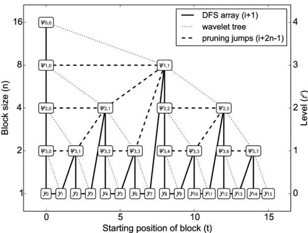
Fig 7. Mapping of waveletsψj,kand data pointsytto tree nodesNℓ,t.Each node is the root of a subtree withn= 2
ℓ
leaves; pruning that subtree yields a block of sizen, starting at positiont. For instance, the nodeN1,6is located at position 13 of the DFS array (solid line), and corresponds to the waveletψ3,3. A block of sizen= 2 can be created by pruning the
subtree, which amounts to advancing by 2n−1 = 3 positions (dashed line), yieldingN3,8at position 16, which is the waveletψ1,1. Thus the number of steps for creating blocks per iteration is at most the number of nodes in the tree, and
The block creation algorithm is simple: upon construction, the tree is converted to depth-first search(DFS) order, which simply amounts to sorting the BFS array according to (kn,j), and can be performed using linear-time algorithms such as radix sort; internally, we imple-mented a different linear-time implementation mimicking tree traversal using a stack. Given a threshold, the tree is then traversed in DFS order by iterating linearly over the array (Fig 7, solid lines). Once the maximum coefficient stored in a node is less or equal to the threshold, a block of sizenis created, and the entire subtree is skipped (dashed lines). As the tree is perfect binary and complete, the next array position in DFS traversal after pruning the subtree rooted at the node at indexiis simply obtained asi+ 2n−1, so no expensive pointer structure needs
to be maintained, leaving the tree data structure a simple flat array. An example of dynamic block creation is given inFig 8.
Once the Gibbs sampler converges to a set of variances, the block structure is less likely to change. To avoid recreating the same block structure over and over again, we employ a tech-nique calledblock structure prediction. Since the different block structures are subdivisions of each other that occur in a specific order for decreasingσ2, there is a simple bijection between the number of blocks and the block structure itself. Thus, for each block sequence length we register the minimum and maximum variance that creates that sequence. Upon entering a new
Fig 8. Example of dynamic block creation.The data is of size T = 256, so the wavelet tree contains 512 nodes. Here, only 37 entries had to be checked against the threshold (dark line), 19 of which (round markers) yielded a block (vertical lines on the bottom). Sampling is hence done on a short array of 19 blocks instead of 256 individual values, thus the compression ratio is 13.5. The horizontal lines in the bottom subplot are the block means derived from the sufficient statistics in the nodes. Notice how the algorithm creates small blocks around the breakpoints, e. g. at t125, which requires traversing to lower levels and thus induces some additional blocks in other parts of the tree (left subtree), since all block sizes are powers of 2. This somewhat reduces the compression ratio, which is unproblematic as it increases the degrees of freedom in the sampler.
doi:10.1371/journal.pcbi.1004871.g008
iteration, we check if the current variance would create the same number of blocks as in the previous iteration, which guarantees that we would obtain the same block sequence, and hence can avoid recomputation.
The wavelet tree data structure can be readily extended to multivariate data of dimensional-itym. Instead of storingmdifferent trees and reconcilingmdifferent block patterns in each iteration, one simply storesmdifferent values for each sufficient statistic in a tree node. Since we have to traverse into the combined tree if the coefficient of any of themtrees was below the threshold, we simply store the largestNℓ,t[d] among the corresponding nodes of the trees,
which means that the block creation can be done inO(T) instead ofO(mT), i. e. the dimension-ality of the data only enters into the creation of the data structure, but not the query during sampling iterations.
Automatic priors
While Bayesian methods allow for inductive bias such as the expected location of means, it is desirable to be able to use our method even when little domain knowledge exists, or large varia-tion is expected, such as the lab and batch effects commonly observed in micro-arrays [91], as well as unknown means due to sample contamination. Since FBG does require a prior even in that case, we propose the following method to specify hyperparameters of a weak prior auto-matically. Posterior samples of means and variances are drawn from a Normal-Inverse Gamma distribution (μ,σ2)*NIΓ(μ0,ν,α,β), whose marginals simply separate into a Normal
and an Inverse Gamma distribution
s2
IGða;bÞ; mN m0;s
2
n
:
Lets2be a user-defined variance (or automatically infered, e. g. from the largest of thefinest detail coefficients, ors^2
MAD), andpthe desired probability to sample a variance not larger than s2. From the CDF of IΓwe obtain
p≔Pðs2 s2Þ ¼G a;
b
s2
GðaÞ ¼Q a; b s2
:
IΓhas a mean forα>1, and closed-form solutions fora2N. Furthermore, IΓhas positive
skewness forα>3. We thus letα= 2, which yields
b¼ s2 W 1 p e þ1
; 0<p1;
whereW−1is the negative branch of the LambertW-function, which is transcendental.
How-ever, an excellent analytical approximation with a maximum error of 0.025% is given in [92], which yields
bs2 2
ffiffiffi b p M1 ffiffiffi b p þ ffiffiffi 2 p
M2bexp M3 ffiffiffi
b p þ1 þb ! ;
b≔ lnp;
M1≔0:3361; M2≔ 0:0042; M3≔ 0:0201:
Since the mean of IΓisab1, the expected variance ofμis
b
nforα= 2. To ensure proper mixing,
we could simply setb
mto the sample variance of the data, which can be estimated from the suffi
contained all states in almost equal number. However, due to possible class imbalance, means for short segments far away fromμ0can have low sampling probability, as they do not
contrib-ute much to the sample variance of the data. We thus defineδto be the sample variance of block means in the compression obtained by^s2
MAD, and take the maximum of those two vari-ances. We thus obtain
m0≔S1
n ; and n¼bmax
nS2 S2 1 n2 ;d
1
:
Numerical issues
To assure numerical stability when working with probabilities, many HMM implementations resort to log-space computations, which involves a considerable number of expensive function calls (exp, log, pow); for instance, on Intel’s Nehalem architecture, log (FYL2X) requires 55 operations as opposed to 1 for adding and multiplying floating point numbers (FADD, FMUL) [93]. Our implementation, which differs from [62] greatly reduces the number of such calls by utilizing the block structure: The term accounting for emissions and self-transitions within the block can be written as
Anwjj 1 ð2πÞnw=2snw
j
exp X
nw
k¼1
ðyw;k mjÞ 2
2s2 j
!
:
Any constant cancels out during normalization. Furthermore, exponentiation of potentially small numbers causes underflows. We hence move those terms into the exponent, utilizing the much stabler logarithm function.
exp X
nw
k¼1
ðyw;k mjÞ 2
2s2 j
þ ðnw 1ÞlogAjj nwlogsj
!
:
Using the block’s sufficient statistics
nw; S1≔
X
nw
k¼1
yw;k; S2≔
X
nw
k¼1 y2
w;k:
the exponent can be rewritten as
EwðjÞ≔ 2m
jS1 S2 2s2
j
þKðnw;jÞ;
Kðnw;jÞ≔ðnw 1ÞlogAjj nw logsjþ m2
j 2s2
j
!
:
K(nw,j) can be precomputed for each iteration, thus greatly reducing the number of expensive function calls. Notice that the expressions above correspond to the canonical exponential fam-ily form exp(ht(x),θi−F(θ) +k(x)) of a product of Gaussian distributions. Hence, equivalent
terms can easily be derived for non-Gaussian emissions, implying that the same optimizations can be used in the general case of exponential family distributions: Only the dot product of the sufficient statisticst(x) and the parametersθhas to be computed in each iteration and for each block, while the log-normalizerF(θ) can be precomputed for each iteration, and the carrier measurek(x) (which is 0 for Gaussian emissions) only has to be computed once.
To avoid overflow of the exponential function, we subtract the largest such exponents among all states, henceEw(j)0. This is equivalent to dividing the forward variables by
exp max k EwðkÞ
;
which cancels out during normalization. Hence we obtain
~
awðjÞ≔exp EwðjÞ maxk EwðkÞ
X
nw
i¼1
aw 1ðiÞAij;
which are then normalized to
^
awðjÞ ¼ ~awðjÞ
P
ka~wðkÞ
:
Availability of supporting data
The supplemental figures, our simulation data and results are available for download athttps://
zenodo.org/record/46263(DOI:10.5281/zenodo.46263) [94], and are referenced as S1–S7
throughout the text. Additionally, the figures can also be viewed through our website athttp://
schlieplab.org/Supplements/HaMMLET/for convenience. The implementation of HaMMLET
and scripts to reproduce the simulation and evaluation are available athttps://github.com/
wiedenhoeft/HaMMLET/tree/biorxiv, and a snapshot is archived athttps://zenodo.org/record/
46262(DOI:10.5281/zenodo.46262) [95]. The high-density aCGH data [68] is available from
http://www.ncbi.nlm.nih.gov/geo/query/acc.cgi?acc=GSE23949(accession GEO:GSE23949).
Coriell etc. data [77] is available fromhttp://www.ncbi.nlm.nih.gov/geo/query/acc.cgi?acc=
GSE16(accession GEO:GSE16). The simulations of [66] are available from the original
authors’s website athttp://www.cbs.dtu.dk/*hanni/aCGH/. Notice that due to the use of a random number generator by HaMMLET, CBS and our simulations, individual results will dif-fer slightly from the data provided in the supplement.
Acknowledgments
We would like to thank Md Pavel Mahmud for helpful advice.
Author Contributions
Conceived and designed the experiments: JW AS. Performed the experiments: JW. Analyzed the data: JW. Wrote the paper: JW AS EB. Software implementation: EB JW.
References
1. Iafrate AJ, Feuk L, Rivera MN, Listewnik ML, Donahoe PK, Qi Y, et al. Detection of large-scale variation in the human genome. Nature Genetics. 2004 Sep; 36(9):949–51. Available from:http://www.nature.
com/ng/journal/v36/n9/full/ng1416.html. doi:10.1038/ng1416PMID:15286789
2. Feuk L, Marshall CR, Wintle RF, Scherer SW. Structural variants: changing the landscape of chromo-somes and design of disease studies. Human Molecular Genetics. 2006 Apr; 15 Spec No:R57–66. Available from:http://www.ncbi.nlm.nih.gov/pubmed/16651370. PMID:16651370
3. McCarroll SA, Altshuler DM. Copy-number variation and association studies of human disease. Nature Genetics. 2007 Jul; 39(7 Suppl):S37–42. Available from:http://www.ncbi.nlm.nih.gov/pubmed/
4. Wain LV, Armour JAL, Tobin MD. Genomic copy number variation, human health, and disease. Lancet. 2009 Jul; 374(9686):340–350. Available from:http://www.sciencedirect.com/science/article/pii/
S014067360960249X. doi:10.1016/S0140-6736(09)60249-XPMID:19535135
5. Beckmann JS, Sharp AJ, Antonarakis SE. CNVs and genetic medicine (excitement and consequences of a rediscovery). Cytogenetic and Genome Research. 2008 Jan; 123(1–4):7–16. Available from:http://
www.karger.com/Article/FullText/184687. doi:10.1159/000184687PMID:19287134
6. Cook EH, Scherer SW. Copy-number variations associated with neuropsychiatric conditions. Nature. 2008 Oct; 455(7215):919–23. Available from:http://www.nature.com/nature/journal/v455/n7215/full/
nature07458.html. doi:10.1038/nature07458PMID:18923514
7. Buretić-TomljanovićA, TomljanovićD. Human genome variation in health and in neuropsychiatric
dis-orders. Psychiatria Danubina. 2009 Dec; 21(4):562–9. Available from:http://www.ncbi.nlm.nih.gov/
pubmed/19935494. PMID:19935494
8. Merikangas AK, Corvin AP, Gallagher L. Copy-number variants in neurodevelopmental disorders: promises and challenges. Trends in Genetics. 2009 Dec; 25(12):536–44. Available from:http://www.
sciencedirect.com/science/article/pii/S016895250900211X. doi:10.1016/j.tig.2009.10.006PMID: 19910074
9. Cho EK, Tchinda J, Freeman JL, Chung YJ, Cai WW, Lee C. Array-based comparative genomic hybrid-ization and copy number variation in cancer research. Cytogenetic and Genome Research. 2006 Jan; 115(3–4):262–72. Available from:http://www.karger.com/Article/FullText/95923. doi:10.1159/ 000095923PMID:17124409
10. Shlien A, Malkin D. Copy number variations and cancer susceptibility. Current Opinion in Oncology. 2010 Jan; 22(1):55–63.
11. Feuk L, Carson AR, Scherer SW. Structural variation in the human genome. Nature Reviews Genetics. 2006 Feb; 7(2):85–97. Available from:http://www.nature.com/nrg/journal/v7/n2/full/nrg1767.html. doi: 10.1038/nrg1767PMID:16418744
12. Beckmann JS, Estivill X, Antonarakis SE. Copy number variants and genetic traits: closer to the resolu-tion of phenotypic to genotypic variability. Nature Reviews Genetics. 2007 Aug; 8(8):639–46. Available from:http://www.ncbi.nlm.nih.gov/pubmed/17637735. doi:10.1038/nrg2149PMID:17637735
13. Sharp AJ. Emerging themes and new challenges in defining the role of structural variation in human dis-ease. Human Mutation. 2009 Feb; 30(2):135–44. Available from:http://www.ncbi.nlm.nih.gov/pubmed/ 18837009. doi:10.1002/humu.20843PMID:18837009
14. Olshen AB, Venkatraman ES, Lucito R, Wigler M. Circular binary segmentation for the analysis of array-based DNA copy number data. Biostatistics (Oxford, England). 2004 Oct; 5(4):557–572. Avail-able from:http://biostatistics.oxfordjournals.org/content/5/4/557.short. doi:10.1093/biostatistics/ kxh008
15. Venkatraman ES, Olshen AB. A faster circular binary segmentation algorithm for the analysis of array CGH data. Bioinformatics. 2007 Mar; 23(6):657–63. Available from:http://bioinformatics.
oxfordjournals.org/content/23/6/657.short. doi:10.1093/bioinformatics/btl646PMID:17234643
16. Xing B, Greenwood CMT, Bull SB. A hierarchical clustering method for estimating copy number varia-tion. Biostatistics (Oxford, England). 2007 Jul; 8(3):632–53. Available from:http://biostatistics. oxfordjournals.org/content/8/3/632.full. doi:10.1093/biostatistics/kxl035
17. Fridlyand J, Snijders AM, Pinkel D, Albertson DG, Jain AN. Hidden Markov models approach to the analysis of array CGH data. Journal of Multivariate Analysis. 2004 Jul; 90(1):132–153. Available from: http://www.sciencedirect.com/science/article/pii/S0047259X04000260. doi:10.1016/j.jmva.2004.02. 008
18. Garnis C, Coe BP, Zhang L, Rosin MP, Lam WL. Overexpression of LRP12, a gene contained within an 8q22 amplicon identified by high-resolution array CGH analysis of oral squamous cell carcinomas. Oncogene. 2004 Apr; 23(14):2582–6. Available from:http://www.ncbi.nlm.nih.gov/pubmed/14676824. doi:10.1038/sj.onc.1207367PMID:14676824
19. Albertson DG, Ylstra B, Segraves R, Collins C, Dairkee SH, Kowbel D, et al. Quantitative mapping of amplicon structure by array CGH identifies CYP24 as a candidate oncogene. Nature Genetics. 2000 Jun; 25(2):144–6. Available from:http://www.ncbi.nlm.nih.gov/pubmed/10835626. doi:10.1038/75985 PMID:10835626
20. Veltman JA, Fridlyand J, Pejavar S, Olshen AB, Korkola JE, DeVries S, et al. Array-based comparative genomic hybridization for genome-wide screening of DNA copy number in bladder tumors. Cancer Research. 2003 Jun; 63(11):2872–80. Available from:http://www.ncbi.nlm.nih.gov/pubmed/12782593. PMID:12782593
bioinformatics.oxfordjournals.org/content/19/13/1714. doi:10.1093/bioinformatics/btg230PMID: 15593402
22. Pollack JR, Sørlie T, Perou CM, Rees CA, Jeffrey SS, Lonning PE, et al. Microarray analysis reveals a
major direct role of DNA copy number alteration in the transcriptional program of human breast tumors. Proceedings of the National Academy of Sciences of the United States of America. 2002 Oct; 99 (20):12963–8. Available from:http://www.pnas.org/content/99/20/12963.long. doi:10.1073/pnas. 162471999PMID:12297621
23. Eilers PHC, de Menezes RX. Quantile smoothing of array CGH data. Bioinformatics. 2005 Apr; 21 (7):1146–53. Available from:http://bioinformatics.oxfordjournals.org/content/21/7/1146.full. doi:10. 1093/bioinformatics/bti148PMID:15572474
24. Cleveland WS. Robust Locally Weighted Regression and Smoothing Scatterplots. Journal of the Amer-ican Statistical Association. 1979 Apr; 74(368). doi:10.1080/01621459.1979.10481038
25. Beheshti B, Braude I, Marrano P, Thorner P, Zielenska M, Squire JA. Chromosomal localization of DNA amplifications in neuroblastoma tumors using cDNA microarray comparative genomic hybridization. Neoplasia. 2003 Jan; 5(1):53–62. Available from:http://www.ncbi.nlm.nih.gov/pmc/articles/ PMC1502121/. doi:10.1016/S1476-5586(03)80017-9PMID:12659670
26. Polzehl J, Spokoiny VG. Adaptive weights smoothing with applications to image restoration. Journal of the Royal Statistical Society: Series B (Statistical Methodology). 2000 May; 62(2):335–354. Available from:http://onlinelibrary.wiley.com/doi/10.1111/1467-9868.00235/abstract. doi:10.1111/1467-9868. 00235
27. Hupé P, Stransky N, Thiery JP, Radvanyi F, Barillot E. Analysis of array CGH data: from signal ratio to gain and loss of DNA regions. Bioinformatics. 2004 Dec; 20(18):3413–22. Available from:http:// bioinformatics.oxfordjournals.org/content/20/18/3413. doi:10.1093/bioinformatics/bth418PMID: 15381628
28. Wang Y, Wang S. A novel stationary wavelet denoising algorithm for array-based DNA Copy Number data. International Journal of Bioinformatics Research and Applications. 2007; 3(x):206–222. doi:10. 1504/IJBRA.2007.013603PMID:18048189
29. Hsu L, Self SG, Grove D, Randolph T, Wang K, Delrow JJ, et al. Denoising array-based comparative genomic hybridization data using wavelets. Biostatistics (Oxford, England). 2005 Apr; 6(2):211–26. Available from:http://biostatistics.oxfordjournals.org/content/6/2/211. doi:10.1093/biostatistics/kxi004
30. Nguyen N, Huang H, Oraintara S, Vo, A. A New Smoothing Model for Analyzing Array CGH Data. In: Proceedings of the 7th IEEE International Conference on Bioinformatics and Bioengineering. Boston, MA; 2007. Available from:http://ieeexplore.ieee.org/xpls/abs_all.jsp?arnumber=4375683.
31. Nguyen N, Huang H, Oraintara S, Vo A. Stationary wavelet packet transform and dependent Laplacian bivariate shrinkage estimator for array-CGH data smoothing. Journal of Computational Biology. 2010 Feb; 17(2):139–52. Available from:http://online.liebertpub.com/doi/abs/10.1089/cmb.2009.0013. doi:
10.1089/cmb.2009.0013PMID:20078226
32. Huang H, Nguyen N, Oraintara S, Vo A. Array CGH data modeling and smoothing in Stationary Wavelet Packet Transform domain. BMC Genomics. 2008 Jan; 9 Suppl 2:S17. Available from:http://www.ncbi. nlm.nih.gov/pmc/articles/PMC2559881/. doi:10.1186/1471-2164-9-S2-S17PMID:18831782
33. Holt C, Losic B, Pai D, Zhao Z, Trinh Q, Syam S, et al. WaveCNV: allele-specific copy number alter-ations in primary tumors and xenograft models from next-generation sequencing. Bioinformatics. 2013 Nov;p. btt611–. Available from:http://bioinformatics.oxfordjournals.org/content/30/6/768.
34. Price TS, Regan R, Mott R, Hedman A, Honey B, Daniels RJ, et al. SW-ARRAY: a dynamic program-ming solution for the identification of copy-number changes in genomic DNA using array comparative genome hybridization data. Nucleic Acids Research. 2005 Jan; 33(11):3455–3464. Available from: http://nar.oxfordjournals.org/content/33/11/3455. doi:10.1093/nar/gki643PMID:15961730
35. Tsourakakis CE, Peng R, Tsiarli MA, Miller GL, Schwartz R. Approximation algorithms for speeding up dynamic programming and denoising aCGH data. Journal of Experimental Algorithmics. 2011 May; 16:1.1. Available from:http://dl.acm.org/citation.cfm?id=1963190.2063517. doi:10.1145/1963190. 2063517
36. Olshen AB, Venkatraman, ES. Change-point analysis of array-based comparative genomic hybridiza-tion data. ASA Proceedings of the Joint Statistical Meetings. 2002;p. 2530–2535.
37. Picard F, Robin S, Lavielle M, Vaisse C, Daudin JJ. A statistical approach for array CGH data analysis. BMC Bioinformatics. 2005 Jan; 6(1):27. Available from:http://www.biomedcentral.com/1471-2105/6/ 27. doi:10.1186/1471-2105-6-27PMID:15705208
![Fig 2. F-measures of CBS (light) and HaMMLET (dark) for calling aberrant copy numbers on simulated aCGH data [66]](https://thumb-eu.123doks.com/thumbv2/123dok_br/18347273.352657/6.918.303.763.117.482/fig-measures-light-hammlet-calling-aberrant-numbers-simulated.webp)