Population and mutation analysis of Y-STR loci in a sample from the city of São Paulo (Brazil)

Population and mutation analysis of Y-STR loci in a sample

from the city of São Paulo (Brazil)

José A. Soares-Vieira

, Ana E.C. Billerbeck

, Edna S.M. Iwamura

, Berenice B. Mendonca

,

Leonor Gusmão

and Paulo A. Otto

1

Departamento de Medicina Legal, Faculdade de Medicina, Universidade de São Paulo, São Paulo,

SP, Brazil.

2

_{Laboratório de Hormônios e Genética Molecular, 1ª Clínica Médica, Hospital das Clínicas,}

Faculdade de Medicina, Universidade de São Paulo, São Paulo, SP, Brazil.

3

Instituto de Patologia e Imunologia Molecular, Universidade do Porto, Porto, Portugal.

4

Departamento de Genética e Biologia Evolutiva, Instituto de Biociências, Universidade de São Paulo,

São Paulo, SP, Brazil.

Abstract

The haplotypes of seven Y-chromosome STR loci (DYS19, DYS389I, DYS389II, DYS390, DYS391, DYS392, and DYS393) were determined in a sample of 634 healthy Brazilian males (190 adult individuals and 222 father-son pairs). The 412 adults were unrelated, and the 222 father-son pairs had their biological relationship confirmed using autosomal STRs (LR > 10,000). Among the 412 adults, a total of 264 different 7-loci haplotypes were identified, 210 of which were unique. The most frequent haplotype was detected in 31 instances, occurring with a frequency of 7.52%. The haplotype diversity index was calculated as 98.83%. Upon transmission of the 1,554 alleles, in 222 fa-ther-son pairs, six mutations were observed, with an average overall rate of 3.86 x 10-3

per locus. A haplotype with a duplicated DYS389I locus, and another with duplicated DYS389I, DYS389II, and DYS439 loci were detected in both fathers and their respective sons.

Key words:Y-STR population data, São Paulo (Brazil), mutation rates, duplications. Received: March 14, 2008; Accepted: June 9, 2008.

Y-chromosome STR typing has become an important tool in forensic analysis (Betzet al., 2001; Sibilleet al., 2002; Cerriet al., 2003; Shewaleet al., 2003; Shewaleet al., 2004; Delfin et al., 2005; Johnsonet al., 2005). Re-cently, the DNA Commission of the International Society of Forensic Genetics (ISFG) has published guidelines and recomendations concerning the use of Y-STRs polymor-phisms in human identification and kinship analysis (Gus-mãoet al., 2005). According to a recent Brazilian govern-ment census (IBGE), 54% of Brazilians were self-declared as white, 38% as mixed (mulatto), and 6% as black; 2% were classified in other categories that include Orientals and Amerindians, with striking regional differences. For instance, mixed tri-hybrid types are overwhelmingly pre-dominant (almost 100%) in some parts of the northeastern region, whereas whites vastly predominate in the southern

states (almost 100% in some inner regions of the states of Santa Catarina and Rio Grande do Sul). Several studies per-formed in different population samples from Brazil (Costa et al., 2002; Grattapagliaet al., 2005; Cainéet al., 2005;; Carvalho-Silvaet al., 2006; Silvaet al., 2006; Domingues et al., 2007; Palhaet al., 2007) have shown, however, that in spite of this racial melting pot, genes carried on the Y chromosome are almost exclusively of European origin (Iberian, Mediterranean, and Central-European), while analyses of mtDNA variability in Brazilian samples re-vealed that about 60% of the maternal lineages are Amerin-dian and African (Carvalho-Silvaet al., 2006). Therefore, regardless of this intense gene flow and high degree of ge-netic heterogeneity, Y chromosome polymorphisms in Bra-zilian males have a distribution typical of a mixed Euro-pean population. This paper presents data on 7 Y-STR loci

DYS19, DYS389I, DYS389II, DYS390, DYS391,

DYS392, and DYS393 in a Brazilian mixed population sample from the city of São Paulo.

Genetics and Molecular Biology, 31, 3, 651-656 (2008)

Copyright © 2008, Sociedade Brasileira de Genética. Printed in Brazil www.sbg.org.br

Send correpondence to José Arnaldo Soares-Vieira. Departa-mento de Medicina Legal, Faculdade de Medicina, Universidade de São Paulo, Rua Teodoro Sampaio 115, 05405-000, São Paulo, SP, Brazil. E-mail: jasv@usp.br.

Whole blood samples were collected from 634 healthy Brazilian males (190 adult individuals and 222 pairs of fathers and respective sons), under written in-formed consent. The 412 adults were unrelated and the 222 father-son pairs had their biological relationship confirmed by paternity index values larger than 10,000 obtained by means of autosomal STRs typing. DNA was extracted from 5 mL of peripheral blood by a salting-out procedure (Miller et al., 1988), and quantified by spectrometry (Ultrospec III, Pharmacia, Piscataway, NJ, USA). The amplification of

DYS19, DYS389I, DYS389II, DYS390, DYS391,

DYS392 and DYS393 loci was performed according to Kayseret al.(1997), in two multiplex reactions, one triplex (DYS391,DYS392, DYS393), and one tetraplex (DYS19, DYS389I, DYS389II and DYS390). One primer of each pair was labeled with a fluorescent dye. In a final volume of 25µL, 50 ng of genomic DNA was mixed with 200µM of dNTP, 2.0 mM MgCl2, 2.5 U of Taq polymerase (Amer-sham Biosciences, Piscataway, NJ, USA), 2.5 µL of the10X reaction buffer provided by the manufacturer, and with the forward and reverse primers. In the triplex reac-tion, the concentrations of primers were 7.0 pmol for DYS391, 8.5 pmol for DYS392 and 3.0 pmol for DYS393; in the tetraplex reaction, 7.0 pmol for DYS19, 6.0 pmol for DYS389I/II and 4.0 pmol for DYS390. The samples were subjected to 30 cycles of amplification in a 9700 thermal cycler (Applied Biosystems, Foster City, CA). The amplifi-cation conditions were 94 °C, 5 min; 35 cycles of 94 °C 1 min, 55 °C 1 min, and 72 °C 1 min; followed by 72 °C 30 min, and 12 °C until the samples were removed from the

thermal cycler. Fragment size analysis was performed using the GeneScan 2.1 software. Two microliters of the amplification products were mixed with 24 µL of Hi-Di Formamide (Applied Biosystems), 1µL of the size stan-dard TAMRA-350 (triplex reaction) or TAMRA-500 (tetraplex reaction) and subjected to capillary electrophore-sis on the ABI 310 Genetic Analyzer (Applied Biosystems) using POP-4 (performance optimized polymer), filter set C and an injection time of 5 s. The electrophoresis time was 24 min for the triplex reaction and 28 min for the tetraplex reaction. Four samples were reanalyzed using the AmpFlSTR YFiler kit (Applied Biosystems) as recom-mended by the manufacturer. Since Y-STRs are haploid, allele and haplotype frequencies, as well as linkage dis-equilibrium values between pairs of genes at different loci and mutation rates per locus, were estimated by direct counting methods, using computer programs prepared by us. The significance of association measurements [linkage disequilibrium values (ldv) estimated between all possible pairs of alleles belonging to two out of the seven loci here studied] was verified through Fisher exact tests performed on 2x2 contingency tables. All the methods here men-tioned are detailed in standard text-books on statistical and population genetic methodology (Zar, 1999; Weir, 2001; Sham, 2002).

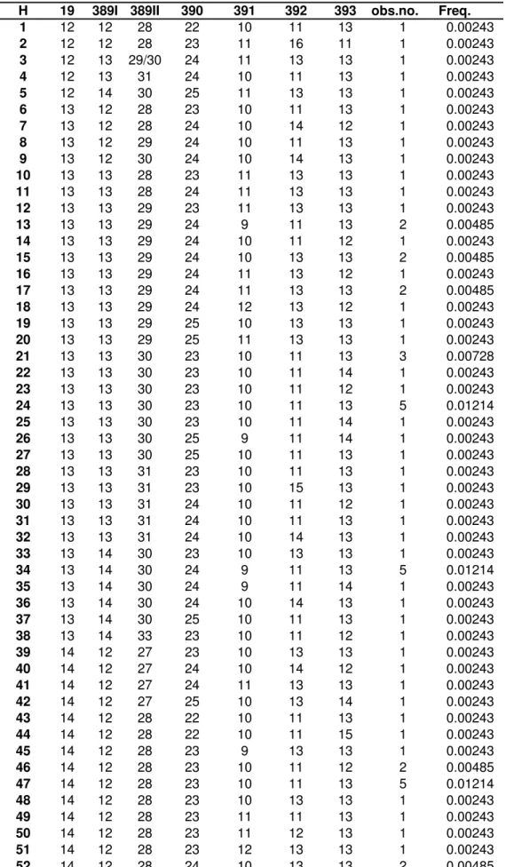
Table 1 lists the observed relative frequencies of dif-ferent Y-STR alleles segregating in each of the seven loci. Table S1 (Supplementary Material) lists the observed abso-lute and relative frequencies of the 7-loci haplotypes among the 412 unrelated adult subjects.

652 Soares-Vieiraet al.

Table 1- Observed relative frequencies of Y-STR alleles segregating at each of the seven loci here reported.

Allele DYS19 DYS389I DYS389II DYS390 DYS391 DYS392 DYS393

8 0.0024

9 0.0558

10 0.0024 0.5073 0.0097

11 0.4053 0.3835 0.0073

12 0.0121 0.1772 0.0316 0.0437 0.1893

13 0.1117 0.6432 0.5073 0.6626

13/14 0.0024

14 0.5655 0.1699 0.0461 0.1165

15 0.2354 0.0049 0.0024 0.0243

16 0.0607 0.0049

17 0.0146

18

19

20

21 0.0704

22 0.0777

23 0.2524

A total of 264 different haplotypes were identified, 210 of which were unique. The most frequent haplotype

(DYS19 14/DYS389I 13/DYS389II 29/DYS390

24/DYS391 11/DYS392 13/DYS393 13) was found in 31 instances (7.52%). The second most frequent haplotype (14/13/29/24/10/13/13), which differed from the previous haplotype by only a single DYS391 repeat, was shared by 14 individuals (3.39%).

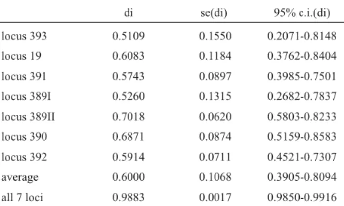
Table 2 lists the estimates of the diversity index ob-tained for each of the 7 Y-STR loci, the average figure cal-culated for these 7 loci and for the set of 7-loci haplotypes, together with their corresponding standard errors and ap-proximate 95% confidence intervals. While diversity indi-ces for isolated loci ranged from 0.51 to 0.70 with an overall average value of 0.60, the 7-loci haplotype diversity index was of the order of 0.99, as expected, since 210/264 (79.5%) of all haplotypes were unique, each occurring with a frequency of about 0.002.

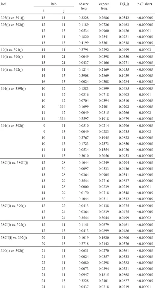
Table 3 lists the results of association tests performed between the genes of possible pairs of Y-STR loci. Since the number of different statistical tests performed was 859, the critical alpha rejection level (for testing the null

hypoth-esis of ldv = 0) was adjusted following Bonferroni’s method, giving a corrected alpha critical value of 0.00006. Therefore, Table 3 lists only the pairs of linked Y-STR loci (out of the 859 tested for linkage disequilibrium) with link-age disequilibrium values [D(i,j)] significantly different from zero at the level of 6 x 10-5or less. As expected, many (if not most) of these very significant values occurred pref-erentially between pairs of contiguous loci.

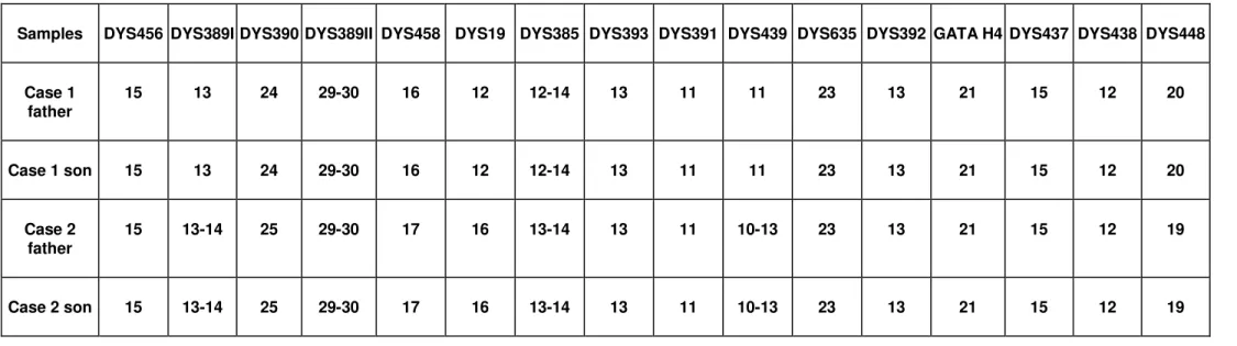
In forensic cases, in which multiple male aggressors are involved, the autosomal STR profiles often provide in-conclusive results. Y-STR markers are being increasingly used as potential tools for distinguishing low levels of male DNA in the presence of excess female DNA, which occurs in many sexual assault samples. Due to the haploid nature of Y-STRs, in cases where multiple males are contributors, the number of donors can be estimated by the presence of additional alleles in a Y chromosome profile, usually being interpreted as an admixture of more than one contributor. The most commonly used Y-STR markers are single-copy loci, with the exception of the DYS385 locus. However, many regions of the Y-chromosome are duplicated or even triplicated in some individuals and this fact can thus com-plicate potential mixture interpretation (Kayseret al., 2000; Bosch and Jobling, 2003; Çakiret al., 2004; Kuriharaet al., 2004; Butleret al., 2005; Diedericheet al., 2005;). The pre-cise estimation of the frequency of duplicated mutated Y-STR alleles is thus very important in forensic genetic analyses, because the presence of multiple peaks can be misinterpreted as mixed profiles (Diedericheet al., 2005). In the present study, one sample had a 7 Y-STR haplotype with double peaks at the DYS389I locus, and another pre-sented a 7 Y-STR haplotype with double peaks at DYS389I and DYS389II. The analysis of these two samples was in-creased to 16 markers, using the AmpF/STR Yfiler Kit, and a double peak was also found in the locus DYS439 of the second sample. Each one of the two pairs of father and son had the same haplotype (Table S2).

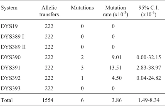
The set of 7 Y-STR loci was typed in 222 father-son pairs. Upon 1,554 allele transmissions, sixde novo

muta-Y-STR loci analysis 653

Table 2- Estimates of Nei’s diversity index (di), with corresponding stan-dard errors [se(di)] and approximate 95% confidence intervals for each in-dividual locus, for their average value, and for the complete 7-loci haplo-types.

di se(di) 95% c.i.(di)

locus 393 0.5109 0.1550 0.2071-0.8148

locus 19 0.6083 0.1184 0.3762-0.8404

locus 391 0.5743 0.0897 0.3985-0.7501

locus 389I 0.5260 0.1315 0.2682-0.7837

locus 389II 0.7018 0.0620 0.5803-0.8233

locus 390 0.6871 0.0874 0.5159-0.8583

locus 392 0.5914 0.0711 0.4521-0.7307

average 0.6000 0.1068 0.3905-0.8094

all 7 loci 0.9883 0.0017 0.9850-0.9916

Table 1 (cont.)

Allele DYS19 DYS389I DYS389II DYS390 DYS391 DYS392 DYS393

25 0.1189

26 0.0049 0.0049

27 0.0121 0.0024

28 0.1408

29 0.4223

29/30 0.0049

30 0.3010

31 0.0947

32 0.0170

654 Soares-Vieiraet al.

Table 3- Results of association tests and estimates of linkage disequilibrium values between possible pairs of Y-STR loci. Only pairs of loci for which the hypothesis of no association was discarded with a probability value less than 0.00006 are shown (see text).

loci hap observ.

freq.

expect. freq.

D(i, j) p (Fisher)

i j

393(i)vs.391(j) 13 11 0.3228 0.2686 0.0542 <0.000005

393(i)vs.392(j) 12 11 0.1189 0.0726 0.0463 <0.000005

12 13 0.0534 0.0960 -0.0426 0.00001

13 11 0.1820 0.2541 -0.0721 <0.000005

13 13 0.4199 0.3361 0.0838 <0.000005

19(i)vs.391(j) 14 11 0.2791 0.2292 0.0499 0.00003

19(i)vs.390(j) 14 21 0.0049 0.0398 -0.0350 <0.000005

15 21 0.0437 0.0166 0.0271 <0.000005

19(i)vs.392(j) 14 11 0.1214 0.2169 -0.0955 <0.000005

14 13 0.3908 0.2869 0.1039 <0.000005

16 13 0.0024 0.0308 -0.0284 <0.000005

391(i)vs.389I(j) 10 12 0.1383 0.0899 0.0485 <0.000005

11 12 0.0316 0.0718 -0.0403 0.00001

10 12 0.0704 0.0394 0.0310 <0.000005

10 1314 0.1699 0.2401 -0.0702 <0.000005

11 12 0.0049 0.0315 -0.0266 0.00002

11 1314 0.2597 0.1918 0.0679 <0.000005

391(i)vs.392(j) 9 11 0.0510 0.0214 0.0296 <0.000005

9 13 0.0049 0.0283 -0.0235 0.00002

10 11 0.2767 0.1945 0.0822 <0.000005

10 13 0.1723 0.2573 -0.0850 <0.000005

11 11 0.0534 0.1554 -0.1020 <0.000005

11 13 0.3010 0.2056 0.0953 <0.000005

389I(i)vs.389II(j) 12 28 0.1044 0.0249 0.0794 <0.000005

12 30 0.0097 0.0533 -0.0436 <0.000005

13 28 0.0364 0.0905 -0.0541 <0.000005

13 29 0.3544 0.2716 0.0827 <0.000005

14 28 0.0000 0.0239 -0.0239 0.00001

14 29 0.0170 0.0718 -0.0548 <0.000005

15 30 0.1044 0.0511 0.0532 <0.000005

389I(i)vs.390(j) 12 22 0.0413 0.0138 0.0275 <0.000005

12 24 0.0364 0.0839 -0.0475 <0.000005

13 24 0.3544 0.3044 0.0499 0.00002

389I(i)vs.392(j) 12 11 0.1141 0.0679 0.0461 <0.000005

12 13 0.0413 0.0899 -0.0486 <0.000005

389II(i)vs.392(j) 29 11 0.1019 0.1620 -0.0600 <0.000005

29 13 0.2718 0.2142 0.0576 <0.000005

390(i)vs.392(j) 21 11 0.0631 0.0270 0.0361 <0.000005

21 13 0.0024 0.0357 -0.0333 <0.000005

22 11 0.0680 0.0298 0.0382 <0.000005

22 13 0.0073 0.0394 -0.0321 <0.000005

24 11 0.0947 0.1815 -0.0868 <0.000005

24 13 0.3228 0.2401 0.0827 <0.000005

tions were observed, one mutation had occurred at the DYS392 locus (14 to 13), two mutations at the DYS390 lo-cus (24 to 23; 22 to 24), and three mutations took place at the DYS391 locus (12 to 10; 12 to 11; 11 to 10) (Table 4). Except for two cases (DYS390 and DYS391), all were sin-gle-step mutations, and only a single mutation occurred during each father-son transmission.

Acknowledgments

This work was partially supported by FAPESP and LIM-HC-FMUSP, Brazil. IPATIMUP is partially sup-ported by Fundação para a Ciência e a Tecnologia, through POCI (Programa Operacional Ciência e Inovação 2010).

References

Betz A, Babler G, Dietl G, Steil X, Weyermann G and Pflug W (2001) DYS STR analysis with epithelial cells in a rape case. Forensic Sci Int 118:126-130.

Bosch E and Jobling MA (2003) Duplications of the AZFa region of the human Y chromosome are mediated by homologous recombination between HERVs and are compatible with male fertility. Hum Mol Genet 12:341-34.

Butler JM, Decker AE, Kline MC and Vallone PM (2005) Chro-mosomal duplications along the Y-chromosome and their potential impact on Y-STR interpretation. J Forensic Sci 50:1-7.

Cainé L, Corte-Real F, Vieira DN, Carvalho M, Serra A, Lopes V and Vide MC (2005) Allele frequencies and haplotypes of 8 Y-chromosomal STRs in the Santa Catarina population of southern Brazil. Forensic Sci Int 148:75-79.

Çakir AH, Celebioglu A and Yardimci E (2004) Y-STR haplo-types in Central Anatolia region of Turkey. Forensic Sci Int 144:59-64.

Carvalho-Silva DR, Tarazona-Santos E, Rocha J, Pena SDJ and Santos FR (2006) Y chromosome diversity in Brazilians: Switching perspectives from slow to fast evolving markers. Genetica 126:251-260.

Cerri N, Ricci U, Sani I, Verzeletti A and de Ferrari F (2003) Mixed stains from sexual assault cases: Autosomal or

Y-Chromosome short tandem repeat? Croat Med J 44:289-292.

Costa NA, Silva B and Moura-Neto RS (2002) Y-chromosome variation in a Rio de Janeiro, Brazil, population sample. Fo-rensic Sci Int 126:254-257.

Delfin FC, Madrid BJ, Tan MP and Ungria MCA (2005) Y-STR analysis for detection and objective confirmation of child sexual abuse. Int J Legal Med 119:158-163.

Diederiche M, Martín P, Amorim A, Corte-Real F and Gusmão L (2005) A case of double alleles at three Y-STR loci: Foren-sic implications. Int J Legal Med 119:223-225.

Domingues PM, Gusmão L, da Silva DA, Amorim A, Pereira RW and de Carvalho EF (2007) Sub Saharan Africa descendents in Rio de Janeiro (Brazil): Population and mutational data for 12 Y-STR loci. Int J Legal Med 121:238-241.

Grattapaglia D, Kalupniek S, Guimarães CS, Ribeiro MA, Diener PS and Soares CN (2005) Y-chromosome STR haplotype diversity in Brazilian populations. Forensic Sci Int 149:99-107.

Gusmão L, Butler JM, Carracedo A, Gill P, Kayser M, Mayr WR, Morling N, Prinz M, Roewer L and Tyler-Smith C (2005) DNA Commission of the International Society of Forensic Genetics (ISFG): An update of the recommendations on the use of Y-STRs in forensic analysis. Int J Legal Med 26:1-10. Johnson CL, Giles RC, Warren JH, Floyd JI and Staub RW (2005)

Analysis of non-suspect samples lacking visually identifi-able sperm using a Y-STR 10- Plex. J Forensic Sci 50:1116-1118.

Kayser M, Cagliá A, Corach D, Fretwell N, Gehrig C, Graziosi G, Heidorn F, Herrmann S, Herzog B, Hidding M,et al.(1997) Evaluation of Y-chromosomal STRs: A multicenter study. Int J Legal Med 110:125-133.

Kayser M, Roewer L, Hedman M, Henke L, Henke J, Brauer S, Kruger C, Krawczak M, Nagy M, Dobosz T,et al.(2000) Characteristics and frequency of germline mutations at microsatellite loci from the human Y chromosome, as re-vealed by direct observation in father/son pairs. Am J Hum Genet 66:1580-1588.

Kurihara R, Yamamoto T, Uchihi R, Li SL, Yoshimoto T, Ohtaki H, Kamiyama K and Katsumata Y (2004) Mutations in 14 Y-STR loci among Japanese father-son haplotypes. Int J Le-gal Med 118:125-131.

Miller SA, Dykes DD and Polesky HF (1988) A simple salt-ing-out procedure for extracting DNA from human nucle-ated cells. Nucleic Acids Res 6:1215.

Palha TJBF, Rodrigues EMR and Santos SEB (2007) Y-chro-mosomal STR haplotypes in a population from the Amazon region, Brazil. Forensic Sci Int 166:233-239.

Sham P (2002) Statistics in Human Genetics. Arnold, London, 290 pp.

Shewale JG, Nasir H, Schneida E, Gross AM, Budowle B and Sinha SK (2004) Y-Chromosome STR system, Y-PlexTM 12, for forensic casework: Development and validation. J Forensic Sci 49:1278-1290.

Shewale JG, Sikka SC, Schneida E and Sinha SK (2003) DNA profiling of azoospermic semen samples from vasectomized males by using Y-Plex TM 6 amplification Kit. J Forensic Sci 48:127-129.

Sibille I, Duverneuil C, Grandmaison GL, Guerrouache K, Teis-sière F, Durigon M and de Mazancourt P (2002) Y-STR DNA amplification as biological evidence in sexually

as-Y-STR loci analysis 655

Table 4- Estimated mutation rates for Y-STR individual loci, together with an overall estimate (average 7-loci figure) and the corresponding 95% binomial exact confidence intervals for each estimate.

System Allelic

transfers

Mutations Mutation rate (x10-3)

95% C.I. (x10-3)

DYS19 222 0 0

DYS389 I 222 0 0

DYS389 II 222 0 0

DYS390 222 2 9.01 0.00-32.15

DYS391 222 3 13.51 2.83-38.97

DYS392 222 1 4.50 0.04-24.82

DYS393 222 0 0

saulted female victims with no cytological detection of sper-matozoa. Forensic Sci Int 125:212-216.

Silva DA, Carvalho E, Costa G, Tavares L, Amorim A and Gusmão L (2006) Y-chromosome genetic variation in Rio de Janeiro population. Am J Hum Biol 18:829-837. Weir BS (2001) Genetic Data Analysis II. Sinauer, Sunderland,

445 pp.

Zar JH (1999) Biostatistical Analysis. Prentice Hall, Upper Sad-dle River, 663 pp.

Internet Resources

Instituto Brasileiro de Geografia e Estatística (IBGE), www.ibge. gov.br (2007).

Supplementary Material

The following online material is available for this ar-ticle:

- Table S1. Observed absolute and relative frequen-cies of STR-Y 7-loci haplotypes.

- Table S2. Y-STR haplotype profiles showing the presence of additional alleles.

This material is available as part of the online article from http://www.scielo.br.gmb.

Associate Editor: Francisco Mauro Salzano

License information: This is an open-access article distributed under the terms of the Creative Commons Attribution License, which permits unrestricted use, distribution, and reproduction in any medium, provided the original work is properly cited.

TABLE S1 – Observed absolute and relative frequencies of STR-Y 7-loci haplotypes.

H 19 389I 389II 390 391 392 393 obs.no. Freq.

1 12 12 28 22 10 11 13 1 0.00243

2 12 12 28 23 11 16 11 1 0.00243

3 12 13 29/30 24 11 13 13 1 0.00243

4 12 13 31 24 10 11 13 1 0.00243

5 12 14 30 25 11 13 13 1 0.00243

6 13 12 28 23 10 11 13 1 0.00243

7 13 12 28 24 10 14 12 1 0.00243

8 13 12 29 24 10 11 13 1 0.00243

9 13 12 30 24 10 14 13 1 0.00243

10 13 13 28 23 11 13 13 1 0.00243

11 13 13 28 24 11 13 13 1 0.00243

12 13 13 29 23 11 13 13 1 0.00243

13 13 13 29 24 9 11 13 2 0.00485

14 13 13 29 24 10 11 12 1 0.00243

15 13 13 29 24 10 13 13 2 0.00485

16 13 13 29 24 11 13 12 1 0.00243

17 13 13 29 24 11 13 13 2 0.00485

18 13 13 29 24 12 13 12 1 0.00243

19 13 13 29 25 10 13 13 1 0.00243

20 13 13 29 25 11 13 13 1 0.00243

21 13 13 30 23 10 11 13 3 0.00728

22 13 13 30 23 10 11 14 1 0.00243

23 13 13 30 23 10 11 12 1 0.00243

24 13 13 30 23 10 11 13 5 0.01214

25 13 13 30 23 10 11 14 1 0.00243

26 13 13 30 25 9 11 14 1 0.00243

27 13 13 30 25 10 11 13 1 0.00243

28 13 13 31 23 10 11 13 1 0.00243

29 13 13 31 23 10 15 13 1 0.00243

30 13 13 31 24 10 11 12 1 0.00243

31 13 13 31 24 10 11 13 1 0.00243

32 13 13 31 24 10 14 13 1 0.00243

33 13 14 30 23 10 13 13 1 0.00243

34 13 14 30 24 9 11 13 5 0.01214

35 13 14 30 24 9 11 14 1 0.00243

36 13 14 30 24 10 14 13 1 0.00243

37 13 14 30 25 10 11 13 1 0.00243

38 13 14 33 23 10 11 12 1 0.00243

39 14 12 27 23 10 13 13 1 0.00243

40 14 12 27 24 10 14 12 1 0.00243

41 14 12 27 24 11 13 13 1 0.00243

42 14 12 27 25 10 13 14 1 0.00243

43 14 12 28 22 10 11 13 1 0.00243

44 14 12 28 22 10 11 15 1 0.00243

45 14 12 28 23 9 13 13 1 0.00243

46 14 12 28 23 10 11 12 2 0.00485

47 14 12 28 23 10 11 13 5 0.01214

48 14 12 28 23 10 13 13 1 0.00243

49 14 12 28 23 11 11 13 1 0.00243

50 14 12 28 23 11 12 13 1 0.00243

51 14 12 28 23 12 13 13 1 0.00243

TABLE S1 (Continued)

H 19 389I 389II 390 391 392 393 obs.no. Freq.

53 14 12 28 24 11 13 13 2 0.00485

54 14 12 28 24 11 14 13 1 0.00243

55 14 12 28 24 12 13 13 1 0.00243

56 14 12 28 27 10 13 13 1 0.00243

57 14 12 29 22 10 11 12 1 0.00243

58 14 12 29 22 10 11 14 1 0.00243

59 14 12 29 23 10 11 12 1 0.00243

60 14 12 29 25 10 13 13 1 0.00243

61 14 12 29 25 11 12 13 1 0.00243

62 14 12 30 22 10 11 13 1 0.00243

63 14 12 30 23 10 12 14 1 0.00243

64 14 13 26 23 10 13 13 1 0.00243

65 14 13 28 23 11 13 13 1 0.00243

66 14 13 28 24 10 13 13 1 0.00243

67 14 13 28 24 11 13 13 4 0.00971

68 14 13 28 24 11 13 14 1 0.00243

69 14 13 28 24 11 14 12 1 0.00243

70 14 13 29 21 11 13 14 1 0.00243

71 14 13 29 22 9 11 12 1 0.00243

72 14 13 29 22 10 11 12 1 0.00243

73 14 13 29 22 10 11 13 1 0.00243

74 14 13 29 23 10 11 12 3 0.00728

75 14 13 29 23 10 13 13 2 0.00485

76 14 13 29 23 11 11 12 3 0.00728

77 14 13 29 23 11 11 13 1 0.00243

78 14 13 29 23 11 12 13 1 0.00243

79 14 13 29 23 11 13 13 4 0.00971

80 14 13 29 24 9 13 13 1 0.00243

81 14 13 29 24 10 11 12 1 0.00243

82 14 13 29 24 10 13 12 7 0.01699

83 14 13 29 24 10 13 13 14 0.03398

84 14 13 29 24 10 14 13 2 0.00485

85 14 13 29 24 11 12 13 1 0.00243

86 14 13 29 24 11 13 12 3 0.00728

87 14 13 29 24 11 13 13 31 0.07524

88 14 13 29 24 11 13 14 2 0.00485

89 14 13 29 24 11 14 12 1 0.00243

90 14 13 29 24 11 14 13 1 0.00243

91 14 13 29 24 12 13 13 1 0.00243

92 14 13 29 25 10 13 13 3 0.00728

93 14 13 29 25 11 11 12 1 0.00243

94 14 13 29 25 11 13 11 1 0.00243

95 14 13 29 25 11 13 13 6 0.01456

96 14 13 29 25 12 13 13 1 0.00243

97 14 13 29 26 10 11 12 1 0.00243

98 14 13 29 26 11 13 12 1 0.00243

99 14 13 30 21 10 11 13 1 0.00243

100 14 13 30 22 10 11 13 1 0.00243

101 14 13 30 22 10 11 14 1 0.00243

102 14 13 30 22 10 13 13 1 0.00243

103 14 13 30 23 10 11 11 1 0.00243

104 14 13 30 23 10 11 12 5 0.01214

105 14 13 30 23 10 13 13 3 0.00728

TABLE S1 (Continued)

H 19 389I 389II 390 391 392 393 obs.no. Freq.

107 14 13 30 23 11 13 13 1 0.00243

108 14 13 30 24 10 10 13 1 0.00243

109 14 13 30 24 10 11 12 2 0.00485

110 14 13 30 24 10 13 12 1 0.00243

111 14 13 30 24 10 13 13 2 0.00485

112 14 13 30 24 10 13 14 1 0.00243

113 14 13 30 24 11 12 13 1 0.00243

114 14 13 30 24 11 13 12 1 0.00243

115 14 13 30 24 11 13 13 7 0.01699

116 14 13 30 24 11 13 14 1 0.00243

117 14 13 30 24 12 13 13 2 0.00485

118 14 13 30 25 10 13 13 1 0.00243

119 14 13 30 25 10 16 13 1 0.00243

120 14 13 30 25 11 13 13 3 0.00728

121 14 13 31 23 10 11 12 1 0.00243

122 14 13 31 23 10 13 13 2 0.00485

123 14 13 31 24 9 11 13 1 0.00243

124 14 13 31 24 11 13 13 1 0.00243

125 14 14 29 23 10 10 14 1 0.00243

126 14 14 29 23 10 13 12 1 0.00243

127 14 14 29 23 10 13 13 1 0.00243

128 14 14 29 23 11 13 13 1 0.00243

129 14 14 29 24 11 14 12 2 0.00485

130 14 14 30 22 10 13 13 1 0.00243

131 14 14 30 23 9 11 13 1 0.00243

132 14 14 30 23 10 11 12 1 0.00243

133 14 14 30 23 10 13 13 1 0.00243

134 14 14 30 23 11 13 12 1 0.00243

135 14 14 30 23 11 13 13 2 0.00485

136 14 14 30 23 12 13 13 1 0.00243

137 14 14 30 24 10 13 12 1 0.00243

138 14 14 30 24 10 13 13 2 0.00485

139 14 14 30 24 11 13 12 1 0.00243

140 14 14 30 24 11 13 13 7 0.01699

141 14 14 30 24 11 13 14 2 0.00485

142 14 14 30 24 11 14 13 2 0.00485

143 14 14 30 24 12 13 13 1 0.00243

144 14 14 30 24 12 13 14 1 0.00243

145 14 14 30 25 10 11 12 1 0.00243

146 14 14 30 25 10 13 12 1 0.00243

147 14 14 30 25 10 13 13 2 0.00485

148 14 14 30 25 11 12 13 1 0.00243

149 14 14 30 25 11 13 13 1 0.00243

150 14 14 31 23 9 11 12 1 0.00243

151 14 14 31 23 9 11 14 1 0.00243

152 14 14 31 23 10 11 13 1 0.00243

153 14 14 31 23 10 13 13 1 0.00243

154 14 14 31 24 11 11 13 1 0.00243

155 14 14 31 24 11 13 13 2 0.00485

156 14 14 31 25 11 11 13 1 0.00243

157 14 14 31 25 11 13 13 1 0.00243

158 14 14 32 23 10 11 13 1 0.00243

159 14 14 32 24 11 13 13 1 0.00243

TABLE S1 (Continued)

H 19 389I 389II 390 391 392 393 obs.no. Freq.

161 14 15 31 25 11 13 13 1 0.00243

162 14 15 32 23 10 13 13 1 0.00243

163 15 10 29 21 10 10 13 1 0.00243

164 15 12 26 21 10 11 13 1 0.00243

165 15 12 27 23 10 13 13 1 0.00243

166 15 12 28 21 10 11 14 1 0.00243

167 15 12 28 22 10 11 13 1 0.00243

168 15 12 28 22 10 11 14 2 0.00485

169 15 12 28 23 10 11 12 1 0.00243

170 15 12 28 23 10 11 14 1 0.00243

171 15 12 28 24 10 11 12 1 0.00243

172 15 12 28 24 10 11 13 2 0.00485

173 15 12 28 24 11 11 12 1 0.00243

174 15 12 28 25 10 11 12 1 0.00243

175 15 12 28 25 11 13 12 1 0.00243

176 15 12 28 25 11 13 13 1 0.00243

177 15 12 29 21 10 11 14 1 0.00243

178 15 12 29 22 10 11 12 1 0.00243

179 15 12 29 22 10 11 14 2 0.00485

180 15 12 29 23 10 11 12 2 0.00485

181 15 12 29 23 10 11 13 1 0.00243

182 15 12 29 23 10 11 15 1 0.00243

183 15 12 29 23 10 12 14 1 0.00243

184 15 12 29 23 10 13 13 1 0.00243

185 15 12 30 22 10 11 14 1 0.00243

186 15 13 28 22 11 11 13 1 0.00243

187 15 13 28 23 10 11 13 1 0.00243

188 15 13 28 25 10 13 13 1 0.00243

189 15 13 28 25 11 13 13 1 0.00243

190 15 13 29 21 10 11 14 1 0.00243

191 15 13 29 22 10 11 13 1 0.00243

192 15 13 29 22 11 13 12 1 0.00243

193 15 13 29 23 9 11 12 3 0.00728

194 15 13 29 23 10 11 12 1 0.00243

195 15 13 29 23 10 11 13 1 0.00243

196 15 13 29 23 10 11 14 1 0.00243

197 15 13 29 23 10 12 14 1 0.00243

198 15 13 29 23 10 13 13 2 0.00485

199 15 13 29 23 10 12 12 1 0.00243

200 15 13 29 23 10 13 13 3 0.00728

201 15 13 29 23 11 13 13 9 0.02184

202 15 13 29 23 11 14 13 2 0.00485

203 15 13 29 23 12 13 14 1 0.00243

204 15 13 29 25 10 13 13 1 0.00243

205 15 13 29 25 11 13 13 1 0.00243

206 15 13 29 25 12 13 13 1 0.00243

207 15 13 30 21 9 11 14 1 0.00243

208 15 13 30 21 10 11 13 1 0.00243

209 15 13 30 21 10 11 14 1 0.00243

210 15 13 30 21 10 11 15 1 0.00243

211 15 13 30 21 11 11 13 1 0.00243

212 15 13 30 21 11 11 14 1 0.00243

213 15 13 30 21 12 11 13 1 0.00243

TABLE S1 (Continued)

H 19 389I 389II 390 391 392 393 obs.no. Freq.

215 15 13 30 23 9 11 12 2 0.00485

216 15 13 30 23 11 13 13 1 0.00243

217 15 13 30 24 10 11 13 1 0.00243

218 15 13 30 24 10 12 15 1 0.00243

219 15 13 30 24 11 13 13 1 0.00243

220 15 13 30 24 11 13 14 2 0.00485

221 15 13 30 24 11 14 13 1 0.00243

222 15 13 31 21 10 10 13 1 0.00243

223 15 13 31 21 10 11 13 3 0.00728

224 15 13 31 21 10 11 15 1 0.00243

225 15 13 31 21 11 11 13 1 0.00243

226 15 13 31 24 10 11 12 1 0.00243

227 15 13 31 24 10 11 13 1 0.00243

228 15 13 31 24 11 13 13 1 0.00243

229 15 13 31 25 10 11 13 1 0.00243

230 15 13 32 22 10 11 14 1 0.00243

231 15 14 29 24 11 13 13 1 0.00243

232 15 14 30 24 11 13 13 1 0.00243

233 15 14 31 22 10 11 14 1 0.00243

234 15 14 31 23 10 12 14 1 0.00243

235 15 14 31 23 10 12 15 1 0.00243

236 15 14 32 24 10 11 12 1 0.00243

237 15 14 32 24 11 13 13 1 0.00243

238 16 12 28 21 10 11 13 1 0.00243

239 16 12 28 22 10 11 13 3 0.00728

240 16 12 28 22 10 11 14 1 0.00243

241 16 12 29 21 10 11 15 1 0.00243

242 16 12 29 21 11 11 13 2 0.00485

243 16 12 29 25 10 11 13 1 0.00243

244 16 13 29 22 10 8 15 1 0.00243

245 16 13 29 23 9 11 12 1 0.00243

246 16 13 29 23 10 12 14 1 0.00243

247 16 13 29 23 11 11 12 1 0.00243

248 16 13 29 23 11 12 14 1 0.00243

249 16 13 29 25 11 12 13 1 0.00243

250 16 13 30 21 10 11 15 1 0.00243

251 16 13 30 23 11 12 13 1 0.00243

252 16 13 30 24 10 11 13 1 0.00243

253 16 13 30 24 10 11 14 1 0.00243

254 16 13 30 24 11 11 13 1 0.00243

255 16 13 30 25 11 11 13 1 0.00243

256 16 13 31 23 10 14 14 1 0.00243

257 16 13 31 24 11 11 13 2 0.00485

258 16 13/14 29/30 25 11 13 13 1 0.00243

259 17 13 28 22 10 11 13 1 0.00243

260 17 13 30 21 10 11 14 1 0.00243

261 17 13 30 24 11 11 13 1 0.00243

262 17 14 30 21 10 11 15 1 0.00243

263 17 14 31 21 10 11 13 1 0.00243

TABLE S2 – Y-STR haplotype profiles showing the presence of additional alleles at DYS389II (case 1) and DYS389I, DYS389II and

DYS439 (case 2), after amplification with the AmpF/STR Yfiler kit.

Samples DYS456 DYS389I DYS390 DYS389II DYS458 DYS19 DYS385 DYS393 DYS391 DYS439 DYS635 DYS392 GATA H4 DYS437 DYS438 DYS448

Case 1 father

15 13 24 29-30 16 12 12-14 13 11 11 23 13 21 15 12 20

Case 1 son 15 13 24 29-30 16 12 12-14 13 11 11 23 13 21 15 12 20

Case 2 father

15 13-14 25 29-30 17 16 13-14 13 11 10-13 23 13 21 15 12 19