Braz. J. Phys. vol.38 número3A

A New Formulation for the Dielectric Tensor for Magnetized Dusty

Plasmas with Variable Charge on the Dust Particles

L. F. Ziebell∗ and R. S. Schneider †

Instituto de F´ısica, Universidade Federal do Rio Grande do Sul, Caixa Postal 15051, CEP: 91501-970, Porto Alegre, RS, Brazil.

M. C. de Juli

Centro de R´adio-Astronomia e Astrof´ısica Mackenzie - CRAAM, Universidade Presbiteriana Mackenzie, Rua da Consolac¸˜ao 896, CEP: 01302-907, S˜ao Paulo, SP, Brazil

R. Gaelzer

Instituto de F´ısica e Matem´atica, Universidade Federal de Pelotas, Caixa Postal 354 - Campus UFPel, CEP: 96010-900, Pelotas, RS, Brazil

(Received on 11 March, 2008)

A kinetic approach to the problem of wave propagation in dusty plasmas, which takes into account the varia-tion of the charge of the dust particles due to inelastic collisions with electrons and ions, is utilized as a starting point for the development of a new formulation, which writes the components of the dielectric tensor in terms of a finite and an infinite series, containing all effects of harmonics and Larmor radius. The formulation is quite general and valid for the whole range of frequencies above the plasma frequency of the dust particles, which were assumed motionless. The formulation is employed to the study of electrostatic waves propagating along the direction of the ambient magnetic field, in the case for which ions and electrons are described by Maxwellian distributions. The results obtained in a numerical analysis corroborate previous analysis, about the important role played by the inelastic collisions between electrons and ions and the dust particles, particularly on the imaginary part of the dispersion relation. The numerical analysis also show that additional terms in the components of the dielectric tensor, which are entirely due these inelastic collisions, play a very minor role in the case of electrostatic waves, under the conditions considered in the present analysis.

Keywords: Langmuir waves; Electrostatic waves; Kinetic theory; Magnetized dusty plasmas; Dust charge fluctuation; Wave propagation

1. INTRODUCTION

The theoretical analysis of waves and instabilities in dusty plasmas have may be traced back to the pioneer work by Bliokh and Yarashenko [1] about waves in Saturn’s rings. Most of the published works utilized fluid theory to describe the dusty plasmas, and only a few of them take into account the collisional charging of the dust particles [2, 3], although the importance of this effect to the propagation and damping of the waves is already well known [4, 5].

Although very important studies have been conducted us-ing an hydrodynamical approach, it must be recognized that the fluid formulation has an important limitation: it can not describe purely kinetic effects such as the Landau damping. This consideration,per se, offers motivation for kinetic stud-ies on dusty plasmas. Moreover, it has been shown that the dust charging process must be included in a kinetic approach, for proper derivation of the wave damping [6]. The reason is basically that the charging process is one of the most conspic-uous and important dissipative processes to occur in a dusty plasma. As argued in Ref. [7], it is not possible to separate the conventional Landau damping and the damping due to the in-teraction of ions and electrons with the dust particles, at least

†_{In Memoriam}

∗_{Electronic address:ziebell@if.ufrgs.br}

for ion-acoustic waves.

assumptions are made.

In the present paper, we resume the use of the same basic kinetic approach, and introduce modifications in the mathe-matical formulation. We obtain expressions for the compo-nents of the dielectric tensor which are written in terms of an infinite and a finite summation, formally incorporating effects of all harmonics and all orders of Larmor radius, keeping ef-fects due to the charging of the dust particles due to inelastic collisions with electrons and ions. The formulation is quite general in terms of frequency range and direction of propaga-tion, and should be very useful for application to the study of wave propagation in dusty plasmas. A preliminary approach to this formulation appeared in the Appendix of Ref. [22], without any details of derivation.

The structure of the paper is the following. In Section 2 we briefly outline the model used to describe the dusty plasma. In Section 3 we present essential features of the kinetic formula-tion which leads to the dielectric tensor for dusty plasmas, and present the new formulation which leads to components of the dielectric tensor expressed in terms of double summations and a small number of basic integrals. In section 4 we discuss the particular case of electrostatic waves propagating along the direction of the ambient magnetic field, and show the deriva-tion of a dispersion reladeriva-tion assuming Maxwellian distribu-tions for the electrons and ions in the equilibrium. In Secdistribu-tions 5 some numerical results obtained from the dispersion relation are presented and discussed. The conclusions are presented in Section 6. Appendixes A and B are included, providing addi-tional details of the derivation of some expressions appearing in the formulation utilized in the present paper. Appendix C shows details of the evaluation of the basic integrals appearing in these expressions, for the case of Maxwellian distributions. Appendix D presents some useful series of Bessel functions, utilized in the derivation of many expressions in the present formulation.

2. THE DUSTY PLASMA MODEL

In our general kinetic formulation we consider a plasma in a homogeneous external magnetic fieldB0=B0ez. In this mag-netized plasma we take into account the presence of spher-ical dust grains with constant radius a and variable charge qd; this charge originates from inelastic collisions between the dust particles and particles of speciesβ(electrons and ions), with chargeq_βand mass m_β. Ions are considered as simply charged, for simplicity.

We consider that the dust grain charging process occurs by the capture of plasma electrons and ions during inelastic col-lisions between these particles and the dust particles. Since the electron thermal speed is much larger than the ion thermal speed, the dust charge becomes preferentially negative. As a cross-section for the charging process of the dust particles, we use expressions derived from the OML theory (orbital motion limited theory) [17, 18].

Another limiting condition is that we focus our attention on weakly coupled dusty magneto-plasmas, in which the electro-static energy of the dust particles is much smaller than their

kinetic energy. This condition is not very restrictive, since a large variety of natural and laboratory dusty plasmas can be classified as weakly coupled [19].

Dust particles are assumed to be immobile, and conse-quently the validity of the proposed model will be restricted to waves with frequency much higher than the characteristic dust frequencies. In particular we consider the regime in which |Ωd| ≪ωpd<ω, whereωpdandΩdare the plasma frequency and the cyclotron frequency of the dust particles, respectively. This condition therefore excludes the analysis of the modes which can arise from the dust dynamics, as the so-called dust-acoustic wave.

3. THE COMPONENTS OF THE DIELECTRIC TENSOR FOR A HOMOGENEOUS MAGNETIZED DUSTY PLASMA

We assume that the distribution function of particles of speciesβ, in a dusty plasma, satisfies Vlasov’s equation ap-pended with a term describing binary inelastic collisions with dust particles,

∂fβ

∂t + p

m_β·∇fβ+qβ ·

E+ p m_βc×B

¸

·∇pfβ

=− Z

σβ

p mβ

(fdfβ−fd0fβ0)dq, (1)

where fd0and fβ0represent respectively the equilibrium dis-tribution functions of dust particles and of particles of species

β, with the subscriptβ=e,i identifying electrons and ions, respectively. The distribution function for the dust particles,

fd, satisfies the following equation,

∂fd

∂t +

∂

∂q[I(r,q,t)fd] =0, (2) where

I(r,q,t) =

_∑

β

Z

d3p q_βσβ(p,q)

p mβ

f_β(r,p,t),

is the current of electrons and ions which charge the dust par-ticles [6]. The presence of the collisional term in these equa-tions assures the possibility of variation of the electric charge of the dust particles, due to the inelastic collisions with parti-cles of speciesβ.

Upon linearization, the perturbed distribution function sat-isfies the following equation,

∂f_β1

∂t + p

m_β·∇fβ1+qβ µ _p

m_βc×B0 ¶

·∇pfβ1+ν0βd(p)fβ1

=−ν1

βd(r,p,t)fβ0−qβ

· E1+

p m_βc×B1

¸

·∇pfβ0, (3)

where

ν0_βd(p) = Z 0

−∞σβ(p,q)

p

ν1_βd(r,p,t) = Z 0

−∞σβ(

p,q) p

m_βfd1(r,q,t)dq, andσβis the charging cross-section, given by [20]

σβ=πa2

µ

1−2qd_apqβ₂mβ

¶ H

µ

1−2qd_apqβ₂mβ

¶ . (4)

After use of Fourier-Laplace transform in the system of equations describing the dusty plasmas, the perturbed distri-bution function can be written as [21]:

ˆ

f_β(p) =fˆ_βC+fˆ_βN, (5) where

ˆ

f_βC=−q_β Z 0

−∞

dτei{k·R−[ω+iν0βd(p)]τ}

×

µ ˆ E+ 1

m_βγβc

p′_×Bˆ ¶

·∇p′fβ0(p⊥,pk),

ˆ f_βN=−

Z 0

−∞

dτei{k·R−[ω+iν0βd(p)]τ}_νˆ

βd(p)fβ0. One notices that ˆfβ

C

has the same formal structure as the per-turbed distribution obtained in the evaluation of the dielectric tensor of a conventional homogeneous magnetized plasma, withω+iν0

βd(p)instead ofωin the argument of the exponen-tial function. This part of the perturbed distribution therefore gives rise to a contribution to the components of the dielectric tensor that corresponds to the usual form of the components obtained for dustless magnetized homogeneous plasma, ex-cept for the modifications due to the presence of the inelastic collision frequencyν0

βd(p), which is related to the equilibrium distribution function of dust particles, as shown by Eq. (3). On the other hand, ˆf_βN features an integrand which is pro-portional to ˆνβd, and which vanishes in the case of dustless plasma. The ˆνβdquantity is the Fourier-Laplace transform of theν1

βdcollision frequency, which is related to inelastic colli-sions with the fluctuating distribution of dust particles.

Using these two contributions to the perturbed distribution function, the dielectric tensor for a magnetized dusty plasma, homogeneous, fully ionized, with identical immobile dust par-ticles and charge variable in time, could be written in the fol-lowing way [21, 22]

εi j=εCi j+εNi j. (6)

One notices that the separation in the two terms appearing in Eq. (6) should not be considered arbitrary, since it is moti-vated by the different nature of the two contributions to the perturbed distribution function depicted by Eq. (5).

The termεC

i jis formally identical, except for theiz compo-nents, to the dielectric tensor of a magnetized homogeneous conventional plasma of electrons and ions, with the resonant denominator modified by the addition of a purely imaginary

term which contains the inelastic collision frequency of dust particles with electrons and ions. For theizcomponents of the dielectric tensor, in addition to the term obtained with the prescription above, there is a term which is proportional to this inelastic collision frequency. Explicit expressions for the componentsεC

i jcan be found in Refs. [21, 22]. The termεN

i jis entirely new and arises only due to the pro-cess of fluctuation of the charge of the dust particles. Its form is strongly dependent on the model used to describe the charg-ing process of the dust particles. The expression for this term can be found in Refs. [21, 22].

As already mentioned, we assume a homogeneous dusty plasma immersed in a homogeneous magnetic field alongz direction, B0=B0ez. Let us also assume waves propagat-ing in an arbitrary direction relative to the ambient magnetic field, with wave vectork=k_⊥e1+k_kez. For the derivation of explicit expressions for the components of the dielectric tensor, we start with the “conventional” part, which in a non-relativistic approximation can be written as follows [21, 22].

εCi j=δi j+

∑

β

X_β n_β0

+∞

∑

n=−∞

Z

d3p p_⊥ϕ0(fβ0) D_nβ

µ_p

k

p_⊥ ¶δiz+δjz

Rn_{i j}β

−δizδjz

∑

β

Xβ

n_β0 Z

d3p

L

(f_β0)pk

p_⊥ (7)

+δjz

∑

β

X_β n_β0

+∞

∑

n=−∞

Z d3p

" iν

0

βd(p)

ω

L

(f_β0) D_nβ

µ_p

k

p_⊥ ¶δiz#

Rn_{i j}β,

where

D_nβ=1−kkpk m_βω−

nΩβ

ω +i ν0

βd(p)

ω ,

Rn_xxβ=n 2

b2

β

J_n2(b_β), R_zznβ=J_n2(b_β),

Rn_xyβ=−Rn_yxβ=in

b_βJn(bβ)J

′

n(bβ),

Rn_xzβ=Rn_zxβ= n b_βJ

2

n(bβ), Rnyyβ=Jn′2(bβ),

Rn_yzβ=−Rn_zyβ=−iJn(bβ)Jn′(bβ),

ν0

βd(p) =

πa2nd0 m_β

¡

p2+C_β¢

p H

¡

p2+C_β¢ ,

ϕ0(fβ0) =

∂f_β0

∂p_⊥− k_k

L

(f_β0) =p_k

∂f_β0

∂p_⊥−p⊥

∂f_β0

∂p_k ,

X_β=ω 2 pβ

ω2 , ω 2 pβ=

4πn_β0q2_β mβ

, Ωβ=

q_βB0 mβc

,

b_β= k⊥p⊥ m_βΩβ

, C_β=−2qβm_aβqd0,

where the subscript β=e,i identifies electrons and ions re-spectively,qd0=εdeZdis the equilibrium charge of the dust particle (positive,εd= +1, or negative,εd=−1) andH de-notes the Heaviside function.

In the evaluation of the componentsεC

i j we need combina-tions of Bessel funccombina-tions, as inJ_n2,J_n′2, andJnJn′, which can be given by Eqs. (D1) of Appendix D. It must be noticed that these quantities, given by Eqs. (D1), depend on|n_|and not onn. However,n appears in other places, as in the resonant denominator. We can writen=s_|n_|, withs=±1, and there-fore the components of the ‘conventional’ part of the dielectric tensor may be written as follows,

εCi j=δi j+δizδjzezz+N

δiz+δjz

⊥ χ

C i j

=δi j+

∑

β

Xβ

n_β0

+∞

∑

n=1s=

∑

±1 Z

d3p p_⊥ϕ0(fβ0) D_snβ

µ_p

k

p_⊥ ¶δiz+δjz

Rsn_{i j}β

+

_∑

β

X_β n_β0

Z

d3p p_⊥ϕ0(fβ0) D_0β

µ_p

k

p_⊥ ¶δiz+δjz

R0_{i j}β

−δizδjz

∑

β

X_β n_β0

Z

d3p

L

(f_β0) p_k

p_⊥ (8)

+δjz

∑

β

X_β n_β0

+∞

∑

n=1s=

∑

±1 Z

d3p "

iν 0

βd(p)

ω

L

(f_β0) D_snβ

µ_p

k

p_⊥ ¶δiz#

Rsn_{i j}β

+δjz

∑

β

X_β n_β0

Z d3p

" iν

0

βd(p)

ω

L

(f_β0) D_0β

µ_p

k

p_⊥ ¶δiz#

R0_{i j}β,

where we have introduced the definition of the χC

i j, and in-troducedN_⊥ as the perpendicular component ofN=ck/ω. Correspondingly,N_kis the parallel component ofN. We have also writtenninstead of|n_|, fom simplicity, sincen_≥1. It is not necessary to write the|n_|because heren is positive and the signsappears explicitly.

Let us define the normalized momentum, u=p/(mαv∗),

wherev_∗is a characteristic velocity, such thatR

d3p f(p) = R

d3u f(u). For instance,v_∗may be the light speedc, or the Alfv´en speedvA, or the ion sound speedcs. Therefore,

p_⊥ϕ0=p_⊥ ·µ

1−kkpk mαω

¶ _∂

∂p_⊥+ k_kp_⊥ mαω

∂ ∂p_k

¸

=u_⊥ ·_³

1−N_k∗u_k´ ∂

∂u_⊥+N

∗

ku⊥

∂ ∂u_k

¸

≡u_⊥L,

L

=p_k ∂

∂p_⊥−p⊥

∂ ∂p_k=uk

∂ ∂u_⊥−u⊥

∂ ∂u_k,

bα=

k_⊥p_⊥ mαΩα =

N_⊥∗u_⊥ sαYα ,

where we have introducedN∗= (v_∗/c)N,Yα=|Ωα|/ω,sα=

sign(Ωα), and also the operatorL. Eq. (8) can be rewritten in

terms of the normalized momentum,

δizδjzezz+N

δiz+δjz

⊥ χCi j=

∑

β

X_β n_β0

+∞

∑

n=1s=

∑

±1 Z

d3u u_⊥L(fβ0)

D

_snβ

µ_u

k

u_⊥ ¶δiz+δjz

Rsn_{i j}β

+

_∑

β

X_β n_β0

Z

d3u u_⊥L(fβ0)

D

_0β

µ_u

k

u_⊥ ¶δiz+δjz

R0_{i j}β

−δizδjz

∑

β

X_β nβ0

Z

d3u

L

(f_β0)uk

u_⊥ (9)

+δjz

∑

β

X_β n_β0

+∞

∑

n=1s=

∑

±1 Z

d3u "

iν 0

βd(u)

ω

L

(f_β0)

D

_snβ

µ_u

k

u_⊥ ¶δiz#

+δjz

∑

β

X_β n_β0

Z d3u

" iν

0

βd(u)

ω

L

(f_β0)

D

_0β

µ_u

k

u_⊥ ¶δiz#

R0_{i j}β,

where

D

_snβ=

Ã

1−N_k∗u_k−sns_βY_β+iν 0

βd(u)

ω

! .

For the evaluation of the ‘new’ contribution, we start from the expression for theεN

i jin Refs. [21, 22], where it is seen that the “new” contribution contains the product of two terms, which in a non-relativistic approximation can be written as follows,

εN

i j=

U

i

S

j, (10)

with

U

_i=−2_aω+i(ν1

ch+ν1)

∑

_β qβ

m2_β

+∞

∑

n=−∞

Z d3p

p_⊥σ′

β(p)p fβ0

ωD_nβ

µ_p

k

p_⊥ ¶δiz

Rn_izβ, (11)

S

_j = −2_ωπa

∑

β

q2_β

+∞

∑

n=−∞

Z d3pν

0

βd(p)

ω

ϕ0(fβ0) D_nβ

µ_p

k

p_⊥ ¶δjz

Rn_{z j}β

−iδjz 2πa

ω

∑

_β q

2

β

+∞

∑

n=−∞

Z d3p

h

ν0

βd(p)/ω i2

D_nβ

L

(f_β0) p_⊥ R

nβ

z j

+δjz 2πa

ω

∑

_β q

2

β

Z d3pν

0

βd(p)

ω

L

(f_β0)

p_⊥ . (12)

where

νch=−

∑

β

q_β m_β

Z

d3pσ′_β(p)p f_β0, (13)

ν1=

∑

β

q_β m_β

+∞

∑

n=−∞

Z d3p

h iν0

βd(p)/ω i

Dnβ

σ′_β(p)p fβ0Rnzzβ. (14)

Moreover,σ′_β(p)≡(∂σβ/∂qd)|qd=−Zde, andσβis the charging cross-section, given by (4).

Effects of charge variation of dust particles occurs in the terms withν0

βd(p)/ω and effects of presence of dust particles, introduced via quasi-neutrality relation (ni06=ne0), occurs in terms withXβ≡ω2pβ/ω2.

Changing variables as in Eq. (8), Eqs. (11), (12), (13), and (14) become

U

_i=−2_a v 2

∗

ω+i(νch+ν1)

∑

_β q_β

+∞

∑

n=−∞

Z

d3uu⊥σ

′

β(u)fβ0u

ωD_nβ µ_u

k

u_⊥ ¶δiz

Rn_izβ,

S

_j = −2πa ω

∑

_β

q2_β m_βv_∗

+∞

∑

n=−∞

Z d3uν

0

βd(u)

ω

L(f_β0) Dnβ

µ_u

k

u_⊥ ¶δjz

Rn_{z j}β

−iδjz 2πa

ω

∑

_β

q2_β m_βv_∗

+∞

∑

n=−∞

Z d3u

h

ν0

βd(u)/ω i2

Dnβ

L

(f_β0) u_⊥ R

nβ

z j

+δjz 2πa

ω

∑

_β

q2_β m_βv_∗

Z d3uν

0

βd(u)

ω

νch=−v∗

∑

β

q_β Z

d3uσ′_β(u)u f_β0,

ν1=v∗

∑

β

q_β

+∞

∑

n=−∞

Z d3u

h iν0

βd(u)/ω i

D_nβ σ

′

β(u)fβ0u Rnzzβ.

ν0_βd(u) =πa 2_n

d0v∗

u Ã

u2+ Cβ m2_βv2

∗

! H

Ã

u2+ Cβ m2_βv2

∗

! .

Using the definition ofC_β, andqd=−Zde,

ν0_βd(u) =πa 2_n

d0v∗

u µ

u2+2Zdeqβ am_βv2

∗

¶ H

µ

u2+2Zdeqβ am_βv2

∗

¶ .

From Eq. (4), we obtain

σβ=π

a2 u2

µ

u2+2Zdeqβ amβcv2_∗

¶ H

µ

u2+2Zdeqβ amβv2_∗

¶ ,

from which we obtainσ′_β,

σ′_β=−πa

u2 2qβ

m_βv2

∗

H µ

u2+2Zdeqβ am_βv2

∗

¶

. (15)

Alternatively, this expression can be written in terms of the inelastic collision frequency,

σ′_β=−1_um2qβ

βv2_∗

1 and0c

µ

u2+2Zdeqβ am_βv2

∗

¶−1

ν0_βd(u). (16)

Using Eq. (15),

U

_i= 4πv 2

∗

ω+i(νch+ν1)

∑

_β q2

β

m_βv2

∗ +∞

∑

n=−∞

Z

d3u fβ0

ωD_nβ u_⊥

u H µ

u2+2Zdeqβ am_βv2

∗

¶ µ_u

k

u_⊥ ¶δiz

Rn_izβ, (17)

S

_j = −2_ωπa

∑

β

q2_β m_βv_∗

+∞

∑

n=−∞

Z d3uν

0

βd(u)

ω

L(f_β0) D_nβ

µ_u

k

u_⊥ ¶δjz

Rn_{z j}β

−iδjz 2πa

ω

∑

_β

q2_β m_βv_∗

+∞

∑

n=−∞

Z d3u

Ã

ν0

βd(u)

ω

!2 1 Dnβ

L

(f_β0) u_⊥ R

nβ

z j

+δjz 2πa

ω

∑

_β

q2_β m_βv_∗

Z d3uν

0

βd(u)

ω

L

(f_β0)

u_⊥ , (18)

νch= (2π)av∗

∑

β

q2_β m_βv2

∗

Z

d3u f_β0 1 uH

µ

u2+2Zdeqβ am_βv2

∗

¶

, (19)

ν1=−i(2π)av_∗

∑

β

q2_β m_βv2

∗ +∞

∑

n=−∞

Z d3u

Ã

ν0

βd(u)

ω

! 1 Dnβ

fβ0 1 uH

µ

u2+2Zdeqβ am_βv2

∗

¶

Rn_zzβ. (20)

Larmor radius terms, leading to general expression which depend on a small number of integrals, which have to be evaluated depending on the equilibrium distribution function. The procedure is as follows. The Bessel functions which appear in theRi j, both in the ‘conventional’ and in the ‘new’ contributions, can be expanded using the expressions which appear in Appendix D, and therefore it is possible to write the components of the dielectric tensor in terms of double series which contains some general integrals. For the ‘conventional’ components,

χxx= 1 z2

∑

β

ω2 pβ

Ω2

∗

1 nβ0

∞

∑

m=1 µ_q

⊥

rβ

¶2(m−1) m

∑

n=−m

n2a(|n_|,m_{− |}n_|)J(n,m,0;f_β0), (21)

χxy=i 1 z2

∑

β

ω2 pβ

Ω2

∗

1 n_β0

∞

∑

m=1 µ

q_⊥ r_β

¶2(m−1) m

∑

n=−m

nma(|n_|,m_{− |}n_|)J(n,m,0;f_β0). (22)

χyx=−i 1 z2

∑

β

ω2 pβ

Ω2

∗

1 n_β0

∞

∑

m=1 µ

q_⊥ r_β

¶2(m−1) m

∑

n=−m

nma(|n_|,m_{− |}n_|)J(n,m,0;f_β0). (23)

χxz= 1 z

v_∗ c

∑

_β

1 rβ

ω2 pβ

Ω2

∗

1 nβ0

∞

∑

m=1 µ_q

⊥

rβ

¶2(m−1) m

∑

n=−m

na(|n_|,m_{− |}n_|)

·

J(n,m,1;f_β0) +iJν(n,m,0;fβ0) ¸

, (24)

χzx= 1 z

v_∗ c

∑

_β

1 r_β

ω2 pβ

Ω2

∗

1 n_β0

∞

∑

m=1 µ_q

⊥

r_β

¶2(m−1) m

∑

n=−m

na(|n_|,m_{− |}n_|)J(n,m,1;f_β0). (25)

χyy= 1 z2

∑

β

ω2 pβ

Ω2

∗

1 n_β0

∞

∑

m=1 µ

q_⊥ r_β

¶2(m−1) m

∑

n=−m

b(|n_|,m_{− |}n_|)J(n,m,0;f_β0), (26)

χyz=−i 1 z

v_∗ c

∑

_β

1 r_β

ω2 pβ

Ω2

∗

1 n_β0

∞

∑

m=1 µ_q

⊥

r_β

¶2(m−1) m

∑

n=−m

a(|n_|,m_{− |}n_|)(m)

·

J(n,m,1;f_β0) +iJ_ν(n,m,0;f_β0)

¸

. (27)

χzy=i 1 z

v_∗ c

∑

_β

1 r_β

ω2 pβ

Ω2

∗

1 n_β0

∞

∑

m=1 µ_q

⊥

r_β

¶2(m−1) m

∑

n=−m

a(|n_|,m_{− |}n_|)(m)J(n,m,1;f_β0). (28)

χzz= v2_∗ c2

∑

β

1 r_β2

ω2 pβ

Ω2

∗

1 n_β0

∞

∑

m=1 µ

q_⊥ r_β

¶2(m−1) m

∑

n=−m

a(|n_|,m_{− |}n_|)

·

J(n,m,2;f_β0) +iJν(n,m,1;fβ0) ¸

, (29)

ezz=−_z12

∑

β

ω2 pβ

Ω2

∗

1 n_β0

Z d3u uk

u_⊥

L

(fβ0) + 1 z2

∑

β

ω2 pβ

Ω2

∗

1 n_β0

a(0,0)

·

J(0,0,2;fβ0) +i Jν(0,0,1;fβ0) ¸

, (30)

where we have defined

J(n,m,h;f_β0)≡z Z

d3u

u_khu_⊥2(m−1)u_⊥L(f_β0) z₋nr_β−q_ku_k+iν˜0

βd

, (31)

Jν(n,m,h;fβ0) = Z

d3u ˜

ν0

βd(u)uh_ku 2(m−1)

⊥ u⊥

L

(fβ0)

z₋nrβ−qkuk+iν˜0βd

with the dimensionless variables

z= ω Ω_∗, qk=

k_kv_∗

Ω_∗ , q⊥=

k_⊥v_∗

Ω_∗ , rβ= Ωβ

Ω_∗, ν˜

0

βd(u) =

ν0

βd(u)

Ω_∗ .

The quantitiesΩ_∗andv_∗are some characteristic frequency and velocity, respectively. Details on these calculations can be found in Appendix A.

Further development can be made in the particular case of Maxwellian distributions for ions and electrons,

fβ0(p) = n_β0 (2π)3/2_p3

β

e−p2/(2p2β)_{, → f}

β0(u) = n_β0 (2π)3/2_u3

β

e−u2/(2u2β)_{, (33)}

wherepβ=pmβTβ, and where we have defineduβ=pβ/p∗=vβ/v∗, withvβ=

q

Tβ/mβ. For these distributions, and indeed for

any isotropic distribution, it is immediate to show that

L

(f_β0) =0, with the consequent vanishing of the integralJν(n,m,h;fβ0). Therefore

χxx= 1 z2

∑

β

ω2 pβ

Ω2

∗

1 n_β0

∞

∑

m=1 µ_q

⊥

r_β

¶2(m−1) m

∑

n=−m

n2a(|n_|,m_{− |}n_|)J(n,m,0;f_β0), (34)

χxy=i 1 z2

∑

β

ω2 pβ

Ω2

∗

1 n_β0

∞

∑

m=1 µ_q

⊥

r_β

¶2(m−1) m

∑

n=−m

nma(|n_|,m_{− |}n_|)J(n,m,0;f_β0). (35)

χxz= 1 z

v_∗ c

∑

_β

1 rβ

ω2 pβ

Ω2

∗

1 nβ0

∞

∑

m=1 µ_q

⊥

rβ

¶2(m−1) m

∑

n=−m

na(|n_|,m_{− |}n_|)J(n,m,1;f_β0). (36)

χyy= 1 z2

∑

β

ω2 pβ

Ω2

∗

1 nβ0

∞

∑

m=1 µ_q

⊥

rβ

¶2(m−1) m

∑

n=−m

b(|n_|,m_{− |}n_|)J(n,m,0;f_β0). (37)

χyz=−i 1 z

v_∗ c

∑

_β

1 rβ

ω2 pβ

Ω2

∗

1 nβ0

∞

∑

m=1 µ_q

⊥

rβ

¶2(m−1) m

∑

n=−m

a(|n_|,m_{− |}n_|)(m)J(n,m,1;f_β0). (38)

χzz= v2_∗ c2

∑

β

1 r2

β

ω2 pβ

Ω2

∗

1 n_β0

∞

∑

m=1 µ_q

⊥

r_β

¶2(m−1) m

∑

n=−m

a(|n_|,m_{− |}n_|)J(n,m,2;f_β0), (39)

χyx=−χxy, χzx=χxz, χzy=−χyz, (40)

ezz= 1 z2

∑

β

ω2 pβ

Ω2

∗

1 nβ0

J(0,0,2;f_β0). (41)

Similar development can be made for the ‘new’ contribution, with details in Appendix B. For general distributions,

U

_x=1 z

1

z+i(ν˜ch+ν˜1)

∑

_β

ω2 pβ

Ω2

∗

1 n_β0

∞

∑

m=1

+m

∑

n=−m µ_q

⊥

r_β ¶2m−1

na(|n_|,m_{− |}n_|)JU(n,m,0,0;fβ0), (42)

U

_y=−i1 z

1

z+i(ν˜ch+ν˜1)

∑

_β

ω2 pβ

Ω2

∗

1 n_β0

∞

∑

m=1

+m

∑

n=−m µ_q

⊥

r_β ¶2m−1

U

_z=1 z

1

z+i(ν˜ch+ν˜1)

∑

_β

ω2 pβ

Ω2

∗

1 n_β0

∞

∑

m=0

+m

∑

n=−m µ_q

⊥

r_β ¶2m

a(|n_|,m_{− |}n_|)JU(n,m,1,0;fβ0), (44)

S

_x=−aΩ∗ 2v_∗ 1 z

∑

_β

ω2 pβ

Ω2

∗

1 n_β0

∞

∑

m=1

+m

∑

n=−m µ_q

⊥

r_β ¶2m−1

na(|n_|,m_{− |}n_|)JνL(n,m,0;fβ0), (45)

S

_y=−iaΩ∗ 2v_∗

1 z

∑

_β

ω2 pβ

Ω2

∗

1 n_β0

∞

∑

m=1

+m

∑

n=−m µ

q_⊥ r_β

¶2m−1

ma(|n_|,m_{− |}n_|)JνL(n,m,0;fβ0), (46)

S

_z =−aΩ∗ 2v_∗ 1 z

∑

_β

ω2 pβ

Ω2

∗

1 nβ0

∞

∑

m=0

+m

∑

n=−m µ_q

⊥

rβ

¶2m

a(|n_|,m_{− |}n_|)

·

JνL(n,m,1;fβ0) +i Jνν(n,m;fβ0) ¸

+aΩ∗ 2v_∗ 1 z

∑

_β

ω2 pβ

Ω2

∗

1

n_β0Jν0(fβ0), (47)

˜

νch= aΩ_∗

2v_∗

∑

_β

ω2 pβ

Ω2

∗

1 n_β0

Jch(fβ0), (48)

˜

ν1=−i aΩ_∗

2v_∗

∑

_β

ω2 pβ

Ω2

∗

1 n_β0

∞

∑

m=0

+m

∑

n=−m µ_q

⊥

r_β ¶2m

a(|n_|,m_{− |}n_|)JU(n,m,0,1;fβ0), (49)

where

JU(n,m,h,l;fβ0) =z Z

d3u Ã

˜

ν0

βd z

!l

f_β0 z₋nr_β−q_ku_k+iν˜0

βd uh_ku2m_⊥

u H

µ

u2+2Zdeqβ am_βv2

∗

¶

. (50)

JνL(n,m,h;fβ0) =z Z

d3u ˜

ν0

βd z

uh_ku2m_⊥−1L(f_β0) z₋nr_β−q_ku_k+iν˜0

βd

, (51)

Jνν(n,m;fβ0) =z Z

d3u Ã

˜

ν0

βd z

!2

u2m_⊥−1

L

(f_β0) z₋nr_β−q_ku_k+iν˜0

βd

, (52)

Jν0(fβ0) = Z

d3u ˜

ν0

βd z

L

₍fβ0)

u_⊥ , (53)

Jch(fβ0) = Z

d3u f_β01 uH

µ

u2+2Zdeqβ amβv2_∗

¶

, (54)

with ˜ν1=ν1/Ω_∗and ˜νch=νch/Ω∗.

For the case of a Maxwellian distribution, the integrals which depend on

L

(f_β0)will vanish, and we obtain

U

_x=1 z

1

z+i(ν˜ch+ν˜1)

∑

_β

ω2 pβ

Ω2

∗

1 n_β0

∞

∑

m=1

+m

∑

n=−m µ_q

⊥

r_β ¶2m−1

U

_y=−i1 z

1

z+i(ν˜ch+ν˜1)

∑

_β

ω2 pβ

Ω2

∗

1 n_β0

∞

∑

m=1

+m

∑

n=−m µ_q

⊥

r_β ¶2m−1

ma(|n_|,m_{− |}n_|)JU(n,m,0,0;fβ0), (56)

U

_z=1 z

1

z+i(ν˜ch+ν˜1)

∑

_β

ω2 pβ

Ω2

∗

1 n_β0

∞

∑

m=0

+m

∑

n=−m µ_q

⊥

r_β ¶2m

a(|n_|,m_{− |}n_|)JU(n,m,1,0;fβ0), (57)

S

_x=−aΩ∗ 2v_∗ 1 z

∑

_β

ω2 pβ

Ω2

∗

1 n_β0

∞

∑

m=1

+m

∑

n=−m µ

q_⊥ r_β

¶2m−1

na(|n_|,m_{− |}n_|)JνL(n,m,0;fβ0), (58)

S

_y=−iaΩ∗ 2v_∗

1 z

∑

_β

ω2 pβ

Ω2

∗

1 nβ0

∞

∑

m=1

+m

∑

n=−m µ_q

⊥

rβ

¶2m−1

ma(|n_|,m_{− |}n_|)JνL(n,m,0;fβ0), (59)

S

_z=−aΩ∗ 2v_∗ 1 z

∑

_β

ω2 pβ

Ω2

∗

1 n_β0

∞

∑

m=0

+m

∑

n=−m µ

q_⊥ r_β

¶2m

a(|n_|,m_{− |}n_|)JνL(n,m,1;fβ0), (60)

with ˜νchand ˜ν1given by Eqs. (48) and (49), respectively.

4. DISPERSION RELATION FOR THE CASE OF ELECTROSTATIC WAVES AND PARALLEL

PROPAGATION

In the case of electrostatic waves (ES waves) and parallel propagation, the dispersion relation is simply given byεzz=0, which can be written as follows,

εC

zz+εNzz=1+ezz+

U

z

S

z=0. From Eq. (41),

ezz= 1 z2

∑

β

ω2 pβ

Ω2

∗

1 n_β0

J(0,0,2;fβ0).

From Eq. (57), forq_⊥=0,

U

_z=1 z

1

z+i(ν˜ch+ν˜1)

∑

_β

ω2 pβ

Ω2

∗

1 n_β0

JU(0,0,1,0;fβ0),

where, from Eq. (48),

˜

νch= aΩ_∗

2v_∗

∑

_β

ω2 pβ

Ω2

∗

1 n_β0

Jch(fβ0),

and from Eq. (49),

˜

ν1=−i aΩ_∗

2v_∗

∑

_β

ω2 pβ

Ω2

∗

1

n_β0JU(0,0,0,1;fβ0). From Eq. (60), forq_⊥=0,

S

_z=−aΩ∗ 2v_∗ 1 z

∑

_β

ω2 pβ

Ω2

∗

1

n_β0JνL(0,0,1;fβ0).

After multiplication byz2and use of the previous expres-sions, the dispersion relation can be written as follows,

" z2+

_∑

β

ω2 pβ

Ω2

∗

1

n_β0J(0,0,2;fβ0) #

−aΩ∗ 2v_∗

"

∑

β

ω2 pβ

Ω2

∗

1 n_β0

JU(0,0,1,0;fβ0) # "

∑

β

ω2 pβ

Ω2

∗

1 n_β0

J_νL(0,0,1;fβ0) #

×

"

z+iaΩ∗ 2v_∗

∑

_β

ω2 pβ

Ω2

∗

1 n_β0

µ

Jch(fβ0)−i JU(0,0,0,1;fβ0) ¶#−1

In the case of Maxwellian distributions for ions and electrons, and using as an approximation the average value of the collision frequency instead of the actual momentum-dependent value, theJintegrals can be evaluated. From Eqs. (C3) and (C6) we obtain

JU(n,m,h,l;fβ0)≃ −u2β

µ_ν˜

β

z ¶l

J(n,m₋1/2,h;f_β0),

JνL(n,m,h;fβ0) = ˜

νβ

z J(n,m,h;fβ0). From Eq. (C2),

J(0,0,1;fβ0) = ( √

2)nβ0 ¡

uβ¢−1ζ0β

h 1+ζˆ0

βZ(ζˆ0β)

i .

J(0,0,2;fβ0) = ( √

2)2nβ0 ¡

uβ¢0ζ0βζˆ0β

h

1+ζˆ0_βZ(ζˆ0_β)i From Eq. (C5),

J(0,−1/2,0;f_β0) = r

π

2nβ0 ¡

u_β¢−3ζ0_βZ(ζˆ0_β),

J(0,−1/2,1;f_β0) =√πn_β0¡ u_β¢−2

ζ0

β

h 1+ζˆ0

βZ(ζˆ0β)

i .

Using these results, and using also Eq. (C7), the dispersion relation becomes

ΛC_+ΛN_{=0, (62)}

where

ΛC₌ "

z2+2

∑

β

ω2 pβ

Ω2

∗

ζ0

βζˆ0β

h 1+ζˆ0

βZ(ζˆ0β)

i #

ΛN=aΩ∗ 2v_∗

√ 2π

"

∑

β

ω2 pβ

Ω2

∗

ζ0_βh1+ζˆ_β0Z(ζˆ0_β)i

# "

∑

β

ω2 pβ

Ω2

∗

˜

νβ

u_βζ 0

β

h

1+ζˆ0_βZ(ζˆ0_β)i

#

×

"

z2₋aΩ∗ 2v_∗

∑

_β

ω2 pβ

Ω2

∗

1 u_β

Ã

−i z r

2

πe

−(uβ_lim)2_/(2u2 β)₊

r

π

2ν˜βζ 0

βZ(ζˆ0β)

!#−1 .

5. NUMERICAL ANALYSIS

We consider the following parameters, which are in the range of parameters of interest for stellar winds: ion temper-atureTi=1.0×104K, ion densityni0=1.0×109cm−3, ion charge numberZi=1.0, and ion massmi=mp, the proton mass. For the radius of the dust particles, we assumea=1.0× 10−4cm. For the classical distance of minimum approach, measured in cm, we use the value λ=1.44×10−7/Ti(eV), whereTi(eV) means the ion temperature expressed in units of eV.

Initially, we estimate the magnitude of the contribution of

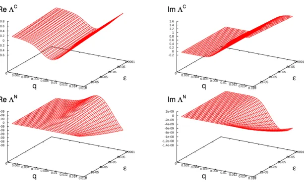
the ‘new’ terms to the dispersion relation of ES waves, and compare it with the ‘conventional’ contribution. In order to do that we assume the occurrence of weakly damped high-frequency oscillations withω≃ωpe. As it is known, waves in this range of frequency are known as Langmuir waves. For normalization purposes, we usev_∗=csandΩ_∗=ωpe0|nd0=0,

whereωpe0|nd0=0is the equilibrium electron plasma frequency

and the ‘new’ contributions to the ES dispersion relation, as defined in Eq. (62), versus normalized wavenumber q and normalized dust densityε. The upper panels of Fig. 1 show respectively, from left to right, the real and the imaginary parts ofΛC_{, while the bottom panels show from left to right the real} and the imaginary parts ofΛN_{. It is seen that for most of the} interval ofq andεdepicted in the figure the real and imagi-nary contributions ofΛN _{are about eight orders of magnitude} smaller than the corresponding contributions ofΛC_.

In Fig. 2 we show the quantities ΛC _andΛN _{vs. q and}

ε, forz= (1×10−2,−2×10−4). This value of frequency well below electron plasma frequency was chosen in order to represent ion-sound waves. For this value ofz, and for the parameters considered in the previous paragraph, the upper panels of Fig. 2 show respectively, from left to right, the real and the imaginary parts ofΛC_{, while the bottom panels show} from left to right the real and the imaginary parts ofΛN_{. As} in the case of the higher frequency Langmuir waves, it is seen that for the interval ofqandεwhere the values ofΛC_andΛN are finite the real and imaginary contributions ofΛN_{are much} smaller than the corresponding contributions ofΛC_.

We also investigate the relative contributions of the ‘con-ventional’ and ‘new’ terms of the dispersion relation in the frequency range of ion-sound waves for electron temperature higher than ion temperature, case in which ion-sound waves are expected to be much more significant than in the case of equal electron and ion temperatures. Figure 3 is obtained for Te/Ti=20, and the other parameters and conditions as in Fig. 2. It shows in the upper panels, from left to right, the real and the imaginary parts ofΛC_{, while the bottom panels show from} left to right the real and the imaginary parts ofΛN_{. As in the} case of Fig. 2, for the interval ofqandεwhere the values of

ΛC _andΛN _{are finite the real and imaginary contributions of}

ΛN _{are much smaller than the corresponding contributions of}

ΛC_.

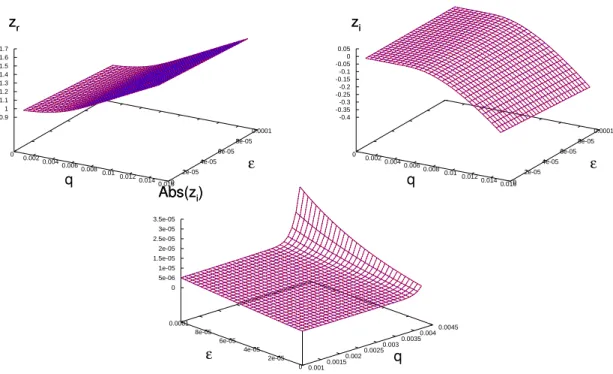
We further explore the role of the dusty plasma and of the ‘new’ contribution for the dispersion relation of ES waves, by consideringTe=Tiand numerically solving Eq. (62) for the frequency range of Langmuir waves. The upper left panel of Fig. 4 shows the value ofzras a function ofqandε, consider-ingεchanging from 0.0 up to 1.0×10−4. The quantityzr ap-pears to be quite insensitive to the presence of the dust. In the upper right panel of Fig. 4 we see the corresponding imagi-nary part. In the scale of the figure, the quantityzialso appears to be insensitive to the presence of the dust. However, an am-plified view of the large wavelength region (smallq), where Landau damping is negligible, appears in the bottom panel of Fig. 4 and shows the occurrence of damping due to the pres-ence of the dust particles. The bottom panel of Fig. 4 shows the absolute value ofzi for values ofq between 1.0×10−3 and 4.2×10−3. It is seen that forε=0.0 values of|zi|due to Landau damping of order 10−6starts to appear only above q_≃0.004. In the region of smallerq(larger wavelengths), the damping rate is zero forε=0.0, but it is seen to increase with the increase of the dust density, along theεaxis. The panel shows that the damping due to the dust particles in the large wavelength region (small values ofq) increases linearly with the dust density, reaching the maximum of|zi| ≃6.0×10−6

for the maximum value ofεconsidered in the calculation. We point out that in Fig. 4 we have plotted the results ob-tained with the dispersion relation given by Eq. (62) using red color. We have also plotted in the same figure, using blue color, the results obtained from a dispersion relation given by

ΛC_{=0, obtained by neglecting the ‘new’ contribution to the} dielectric tensor. The results hardly can be distinguished in the scale of the figure, reflecting the fact that for the range of frequency and for the parameters utilized the effect of the ‘new’ contribution is negligible in the dispersion relation of ES waves. In a monochromatic version of Fig. 4 the two dif-ferent results can hardly be distinguished. In a color version of Fig. 4, the two different results appear so close that the curves feature a light purple color, result of the superposition of the results featured with red color and the results featured with blue color.

6. CONCLUSIONS

In the present paper we have addressed the problem of wave propagation in dusty plasmas, starting from a kinetic formu-lation which takes into account the incorporation of electrons and ions to the dust particles due to inelastic collisions, and used this formulation in order to develop general expressions for the components of the dielectric tensor for magnetized dusty plasmas, valid for general direction of propagation. The dielectric tensor can be divided into two parts, one which is denominated ‘conventional’ and which is formally similar to the dielectric tensor of dustless plasmas, and another which appears due to occurrence of the inelastic collisions between electrons and ions and the dust particles, and which is denom-inated as the ‘new’ contribution. In the formulation developed here, both the ‘conventional’ and the ‘new’ contribution were written in terms of double series, formally containing all har-monic and Larmor radius contributions. These general expres-sions depend on a small number of integrals which depend on the distribution function. We believe that this formulation can be useful for the study of wave propagation in dusty plasmas under a large variety of conditions and parameters.

As further development, we have considered the case of Maxwellian distributions for ions and electrons, and intro-duced an approximation which uses the average value of the inelastic collision frequencies of electrons and ions with the dust particles, instead of the actual momentum dependent ex-pressions. This approximation was adopted in order to arrive at a relatively simple estimate of the effect of the charging of dust particles due to collisions with electrons and ions, ef-fect which is frequently neglected in analysis of the disper-sion relation for waves in dusty plasmas. After the choice of Maxwellian distributions, and after the approximation replac-ing a fixed average value instead of the momentum dependent collision frequencies, the integrals which appear in the com-ponents of the dielectric tensor can be written in terms of the very familiarZ function, whose analytic properties are well known. The formulation therefore becomes specially suitable for numerical analysis.

0 _0.002 0.004

0.006 _0.008 0.01

0.012 _0.014 0.016 0

2e-05 4e-05

6e-05 8e-05

0.0001 -0.6

-0.4 -0.2 0 0.2 0.4 0.6 0.8 Re ΛC

q

ε

Re ΛC

0 _0.002 0.004

0.006 _0.008 0.01

0.012 _0.014 0.016 0

2e-05 4e-05

6e-05 8e-05

0.0001 -0.2

0 0.2 0.4 0.6 0.8 1 1.2 1.4 1.6 Im ΛC

q

ε

Im ΛC

0 0.002 _0.004

0.006 0.008

0.01 _0.012 0.014

0.016 0 2e-05

4e-05 6e-05

8e-05 0.0001 -1.2e-08

-1e-08 -8e-09 -6e-09 -4e-09 -2e-09 0 2e-09 4e-09 6e-09

Re ΛN

q

ε

Re ΛN

0 0.002 _0.004

0.006 0.008

0.01 _0.012 0.014

0.016 0 2e-05

4e-05 6e-05

8e-05 0.0001 -1.4e-08

-1.2e-08 -1e-08 -8e-09 -6e-09 -4e-09 -2e-09 0 2e-09

Im ΛN

q

ε

Im ΛN

FIG. 1: (upper left) Real part of the “conventional” contribution to the dispersion relation, vs. qandε=nd/ni0; (upper right) imaginary part of the “conventional” contribution; (bottom left) Real part of the “new” contribution; (bottom right) imaginary part of the “new” contribution; z= (1.1,−0.001), in the range ofLwaves.

0 _0.002 0.004

0.006 _0.008 0.01

0.012 _0.014 0.016 0

2e-05 4e-05

6e-05 8e-05

0.0001 0

0.01 0.02 0.03 0.04 0.05 0.06 Re ΛC

q

ε

Re ΛC

0 _0.002 0.004

0.006 _0.008 0.01

0.012 _0.014 0.016 0

2e-05 4e-05

6e-05 8e-05

0.0001 0

0.002 0.004 0.006 0.008 0.01 0.012 0.014

Im ΛC

q

ε

Im ΛC

0 0.002 _0.004

0.006 0.008

0.01 _0.012 0.014

0.016 0 2e-05

4e-05 6e-05

8e-05 0.0001 0

1e-06 2e-06 3e-06 4e-06 5e-06 6e-06 7e-06 8e-06 9e-06 1e-05

Re ΛN

q

ε

Re ΛN

0 0.002 _0.004

0.006 0.008

0.01 _0.012 0.014

0.016 0 2e-05

4e-05 6e-05

8e-05 0.0001 0

1e-06 2e-06 3e-06 4e-06 5e-06 6e-06 7e-06

Im ΛN

q

ε

Im ΛN

0 0.002

0.004 0.006 _0.008

0.01 0.012 _0.014

0.016 0 2e-05

4e-05 6e-05

8e-05 0.0001 -0.01

0 0.01 0.02 0.03 0.04 0.05 0.06 Re ΛC

q

ε

Re ΛC

0 0.002

0.004 0.006 _0.008

0.01 0.012 _0.014

0.016 0 2e-05

4e-05 6e-05

8e-05 0.0001 -0.002

0 0.002 0.004 0.006 0.008 0.01 0.012 0.014

Im ΛC

q

ε

Im ΛC

0 0.002 _0.004

0.006 0.008 _0.01

0.012 0.014

0.016 0 2e-05

4e-05 6e-05

8e-05 0.0001 -5e-07

0 5e-07 1e-06 1.5e-06 2e-06 2.5e-06 3e-06 3.5e-06

Re ΛN

q

ε

Re ΛN

0 0.002 _0.004

0.006 0.008 _0.01

0.012 0.014

0.016 0 2e-05

4e-05 6e-05

8e-05 0.0001 -5e-07

0 5e-07 1e-06 1.5e-06 2e-06 2.5e-06

Im ΛN

q

ε

Im ΛN

FIG. 3: Components of the dispersion relation for the range ofSwaves, forz= (1.0×10−2,−2.0×10−4), using the same conventions as those used in the previous figure, and the same parameters, exceptTe/Ti=20.

0 _0.002 0.004

0.006 _0.008 0.01

0.012 0.014 _0.016 0

2e-05 4e-05

6e-05 8e-05

0.0001 0.9

1 1.1 1.2 1.3 1.4 1.5 1.6 1.7 z_r

q

ε

z_r

0 _0.002 0.004

0.006 _0.008 0.01

0.012 0.014 _0.016 0

2e-05 4e-05

6e-05 8e-05

0.0001 -0.4

-0.35 -0.3 -0.25 -0.2 -0.15 -0.1 -0.05 0 0.05 z_i

q

ε

z_i

0.001 0.0015 0.002 0.0025

0.003 0.0035 0.004 0.0045

0 2e-05 4e-05 6e-05 8e-05 0.0001

0 5e-06 1e-05 1.5e-05 2e-05 2.5e-05 3e-05 3.5e-05

Abs(z_i)

q

ε

Abs(z_i)