Rev. adm. empres. vol.57 número5

ROBERT EUGENE LOBEL

relobel@gmail.com

Master in Computer Science from Pontifícia Universidade Católica do Rio de Janeiro – Rio de Janeiro – RJ, Brazil

MARCELO CABUS KLOTZLE

klotzle@iag.puc-rio.br Professor at Pontifícia Universidade Católica do Rio de Janeiro, Centro de Ciências Sociais – Rio de Janeiro – RJ, Brazil

PAULO VITOR JORDÃO DA GAMA SILVA

rjdagama@hotmail.com PhD Student in Business Administration from Pontifícia Universidade Católica do Rio de Janeiro – Rio de Janeiro – RJ, Brazil

ANTONIO CARLOS FIGUEIREDO PINTO

figueiredo@iag.puc-rio.br Professor at Pontifícia Universidade Católica do Rio de Janeiro, Instituto de Administração e Gerencia – Rio de Janeiro – RJ, Brazil

ARTICLES

Submitted 12.20.2016. Approved 05.23.2017

Evaluated by double-blind review process. Scientiic Editor: Danilo Braun Santos

PROSPECT THEORY: A PARAMETRIC

ANALYSIS OF FUNCTIONAL FORMS IN BRAZIL

Teoria do prospecto: Uma análise paramétrica de formas funcionais no Brasil

Teoría prospectiva: Análisis paramétrico de formas funcionales en Brasil

ABSTRACT

This study aims to analyze risk preferences in Brazil based on prospect theory by estimating the risk aversion parameter of the expected utility theory (EUT) for a select sample, in addition to the value and probability function parameter, assuming various functional forms, and a newly proposed value func-tion, the modiied log. This is the irst such study in Brazil, and the parameter results are slightly diferent from studies in other countries, indicating that subjects are more risk averse and exhibit a smaller loss aversion. Probability distortion is the only common factor. As expected, the study inds that behavioral models are superior to EUT, and models based on prospect theory, the TK and Prelec weighting function, and the value power function show superior performance to others. Finally, the modiied log function proposed in the study its the data well, and can thus be used for future studies in Brazil.

KEYWORDS | Behavioral inance, prospect theory, value function, weighting function, Brazil.

RESUMO

Este estudo teve o objetivo de analisar as preferências ao risco no Brasil seguindo os preceitos da Teoria do Prospecto. Para tal, foi estimado o parâmetro de aversão ao risco da Teoria da Utilidade Esperada para uma amostra selecionada, e foram sugeridos os parâmetros da função e probabilidade, supondo diversas formas funcionais e uma nova função de valor – a log modificada. Este foi o primeiro estudo realizado no Brasil para a estimação de tais valores. Os resultados mostraram parâmetros ligeiramente diferentes daqueles encontrados em estudos realizados em outros países, apontando que, no caso da amostra estudada, os indivíduos são mais avessos ao risco e exibem uma menor aversão à perda. A dis-torção de probabilidade é o único elemento semelhante ao de outros países. Como esperado, o estudo constatou a superioridade dos modelos comportamentais em relação à Teoria da Utilidade Esperada (TUE). Além disso e correspondente às expectativas, o desempenho de modelos baseados na Teoria do Prospecto, TK, Função de Ponderação de Prelec e Função Valor Potencia foi superior aos demais. Por fim, a função de log modificada sugerida no estudo encaixa-se bem nos dados e pode assim ser aplicada em futuros estudos no Brasil.

PALAVRAS-CHAVE | Finanças comportamentais, teoria do prospecto, função valor, função peso, Brasil.

RESUMEN

El presente estudio tiene como objeto analizar las preferencias de riesgo en Brasil con base en la teoría prospectiva al estimar el parámetro de aversión al riesgo de la teoría de la utilidad esperada (EUT por sus siglas en inglés) para una muestra seleccionada, además del parámetro de la función de valor y probabilidad, asumiendo diversas formas funcionales, y una función de valor recientemente propuesta, el log modificado. Este es el primer estudio de su clase en Brasil y los resultados de los parámetros difie-ren levemente de estudios realizados en otros países, indicando que los individuos son más reacios al riesgo y muestran una menor aversión a pérdidas. La distorsión de probabilidades es el único factor en común. Como se previó, el estudio muestra que los modelos comportamentales son superiores a la EUT y los modelos basados en la teoría prospectiva, la función de ponderación de TK y Prelec, y la función de potencia de valor muestran desempeño superior a otros. Por último, la función de log modificado propuesta en el estudio se adecua bien a los datos y, por lo tanto, puede usarse para futuros estudios en Brasil.

PALABRAS CLAVE | Finanzas comportamentales, teoría prospectiva, función de valor, función de ponde-ración, Brasil.

INTRODUCTION

For many years traditional inance models were based on neo-classical economics, which is based on certain assumptions about the behavior of decision-makers, such as rational preferences, the maximization of expected utility, and the possession of complete information at any given moment.

The modeling of investor preferences is based on the so-called expected utility theory (EUT), irst developed by von Neuman and Morgenstern (von Neumann & Morgenstern, 1944), and used by Markowitz to structure his mean-variance model

(Markowitz, 1952). However, recent behavioral inance studies have found evidence that prospect theory (Kahneman & Tversky, 1979) and cumulative prospect theory (Tversky & Kahneman, 1992)

provide a better description of investor choice than Markowitz’s mean-variance model.

Prospect theory has been used, amongst other things, to explain the low participation of individual investors in the stock market, high trading intensity in capital markets (Gomes, 2005), investor preference for returns with positive asymmetric distributions (Barberis & Huang, 2008) and the stock market’s risk premium and volatility (Barberis, Huang, & Santos, 2001). To date, most studies have used samples composed of students to test decision making from a prospect theory standpoint (Stott, 2006, Abdellaoui, Bleichrodt, & L’Haridon, 2008, Harrison & Rutström, 2009; Zeisberger, Vrecko, & Langer, 2012).

In all these studies, various values and weighting functions were estimated using parametric and/or non- parametric techniques. The majority of these studies used samples from developed countries and, on a smaller scale, from developing countries. Thus, there is a lack of studies that model value and weighting curves in developing countries, in particular Brazil.

This study seeks to contribute to the study of behavioral inance in Brazil by attempting to model individuals’ decision-making using prospect theory to estimate parameters. Thus, analyses will be performed on 27 models constructed using nine diferent functions, and a newly proposed value function, the modiied log.

THEORETICAL REFERENCES

Developed by Bernoulli in 1738 (Bernoulli, 1954), EUT only became widely known in 1944 when von Neumann and Morgenstern (1944)

demonstrated that the theory can be systematically explained by a set of basic axioms of choice. For a long time, EUT was the basis for the analysis of the decision-making process in situations

involving risk, and was the cornerstone of classical economics. However, beginning with the famous Allais paradox (Allais, 1953)

and later the Ellsberg paradox (Ellsberg, 1961), it gradually became evident that an individual’s decision-making process does not follow an absolutely rational model. This led to the development of the non-EUT, which embraces the prospect theory developed by Kahneman and Tversky (Kahneman & Tversky, 1979). Non-EUT refers to the set of alternative models of decision making that attempt to accommodate the systematic violations of many of the key assumptions of the expected utility model of choice under uncertainty (Machina, 2008).

Prospect theory presents an alternative to the EUT by introducing an observed probability distortion function (“weighting function”) and a value function that expresses the variation of wealth. Over the past 30 years, several variants of this theory have been proposed, such as the cumulative prospect theory developed by Tversky and Kahneman (1992) and the normalized prospect theory (Rieger & Wang, 2008, Karmarkar, 1979 and Karmarkar, 1978). These alternatives encompass variations in theoretical modeling and the weighting and value functions.

Utility theory

Gerber and Pafum (1998) summarized the various types of utility functions used in modern inance theory. The utility function is typically represented by a power function, as in eq. (1) below.

,

u x

^ h

=

_d

1

x

where δ ≤ 1.The Arrow-Pratt absolute risk aversion coeicient (Wakker, 2008), is deined in eq. (2).

,

RA x

^ h

=

1

-

_x

d

where x represents inal wealth (i.e., initial wealth plus the inal value of the lottery). The δ parameter can be interpreted as the relative risk aversion coeicient (Palacios-Huerta & Serrano, 2006 and Holt & Laury, 2002).

(

) (

)

(

),

EUT

=

1

-

p u A

+

w

+

pu B

+

w

where A_i and B_i are the results of lottery i (A_i < B_i), p is the probability of obtaining the highest result B_i, u is the utility function, and w is initial wealth. In the case of a lottery with

x_i results (already incorporating initial wealth), each one with probability p_i, eq. (3) can be generalized and deined as in eq. (3a) below.

( )

EUT

p u x

i n

1

=

=

|

Prospect theory and its variants

Kahneman and Tversky (1979) proposed an alternative model for describing choice under uncertainty with the propspect theory. In prospect theory, the value function (v(x)) replaces the utility function in the EUT. According to Kahneman and Tversky (1979), the value function (v) can be parameterized as a power function, as follows in eq. (4).

( )

,

v

( ) , ,

x x

x x

0 0

a

=

$ m

- - b

#

where α and β measure the curvature of the value function for gains and losses respectively and λ is the loss aversion coeicient.

A second characteristic of the prospect theory refers to the estimation of probabilities of the occurrence of events.Whereas the EUT uses simple probabilities, prospect theory uses decision weights. Tversky and Kahneman (1992) deined and calibrated a weighting function based on experiments, which assigns a weight w (p) to each probability p. This weight,in turn, relects the impact of p on the prospect’s total value. In most cases, the sum of the weights is less than 1 (i.e., w(p) + w(p-1) < 1). The weighting function (w(p)) is parametrized as follows in eq. (5).

( )

(

(

) )

,

w p

p

p

p

1

=

+

-c c _c

c

(5)

where γ ε (0.1). A characteristic of this weighting function is that it assigns a higher weight to low probabilities and a lower weight to high probabilities. The value of γ will determine the degree of over or under assessment of the weights assigned to absolute probabilities. The lower the parameter, the greater the distortion of probabilities given that most of the function’s range lie below the 45-degree line.

Originally, the weighting function permitted the existence of diferent parameters in the gain and loss area (Tversky & Kahneman, 1992). However, as previous studies estimated very similar parameters in the gain and loss area (Tversky & Kahneman, 1992, Camerer & Ho, 1994 and Tversky & Wakker, 1995), it is common to model w(p) estimating only one γ for both gains and losses (Rieger, Wang & Hens, 2011).

According to prospect theory, the value of a lottery prospect with x_i results each with probability p_i,(Rieger & Bui, 2011), can be deined as in eq. (6) below.

( , )

( ) ( )

( ) ( )

v x p

=

w p v x

+

w p v x

+

g

+

( ) ( ),

w p v x

g

+

+

where w(p) is the weighting function and v(x) the value function.

Tversky and Kahneman (1992) presented a new version of the prospect theory, which they called cumulative prospect theory. The main diference between the two is that the latter includes cumulative instead of individual probability distortions to include non-linear preferences (rank dependence), and satisies the stochastic dominance condition.

Similar to eq. (6), we can deine the value of a lottery prospect with x_i results each with probability p_i as deined in eq. (7) below.

( , )

( ) ( ),

v x p

w p v x

i n

1

=

|

where v(x) is the value function as in prospect theory, and w(p)

is the subjective weighting function derived from the probabilities of results (Rieger & Bui, 2011), as deined in eq. (8) below.

( )

(

)

(

)

w p

=

w p

+

g

+

p

-

w p

+

g

+

p

A variant of the prospect theory, known as normalized prospect theory, was perfected by Rieger and Wang (2008), drawing on Karmarkar (1978). The value of the lottery prospect with x_i results each with probability p_i is deined as in eq. (9) below.

( , )

( )

( ) ( )

v x p

w p

w p v x

i i n i i i n 1 1

=

|

|

In this case, the prospect function is normalized by the sum of subjective probabilities. This normalization makes it possible to extend prospect theory to non-discrete lotteries.

Additional functions

Over the years, various types of functions have been suggested within the theoretical and empirical formulation of prospect theory, involving diferent speciications of the value and weighting functions.

Regarding the value function, it should be highlighted that, in addition to the power function used by Kahneman and Tversky (1979) and deined in eq. (4), the exponential and quadratic functions are also cited in the literature (Rieger & Bui, 2011).

The logarithmic function (Köbberling & Wakker, 2005) is deined as in eq. (10) below.

( )

( .

(

)

,

,

( .

(

)

ln

ln

v

x

x

x

x

1 0001

1

0

0

1 0001

1

1

$

b

b

a

a

=

-+

-+

Z

[

\

]]]

]]

]]]

]]]

Although the logarithmic function is often cited (Camerer & Ho, 1994, Fishburn & Kochenberger, 1979) and generally considered to be the irst utility function developed by Bernoulli in the 18th century (Stott, 2006), it has also been criticized because of its inability to diferentiate high values of x due to its steeper slope. It only functions well with high values if α and β are relatively small (Bui, 2009).

The quadratic function has played an important role in inance. Its advantage lies in its ability to price the value of a prospect solely in its mean and variance, widely used in inance, mainly in asset pricing (Stott, 2006). The quadratic function is deined as follows in eq. (11).

( )

X

₍

,

_),

v

x

x

x

x

x x

0

0

1

$

m

b

a

=

(

-

₊

The exponential function, in turn, is deined as follows in eq. (12).

( )

(

),

,

X

v

e

x

e

x

1

0

1

0

1

$

m

=

-

-(

The weighting function also exhibits some functional variants in addition to those developed by Tversky and Kahneman (1992) and deined in eq. (5). We cite the functions proposed by

Karmarkar (1978), Karmarkar (1979) and Prelec (1998). Karmarkar’s weighting function (Karmarkar, 1978; Karmarkar, 1979) is deined in eq. (13) below.

( )

(

(

) )

p

w

p

p

p

1

=

+

-

Meanwhile, Prelec (1998) proposed the invariant composite form of the weighting function, which is characterized below in eq. (14).

( )

p

exp

( (

ln

( ))

w

₌

_{- -}

p

This function makes it possible to explain distortions such as the common consequence efect (Allais, 1953) more consistently. Probability functions with two parameters have also been developed; among the most important are Goldstein and Einhorn (1987) and Prelec’s (1998) functions.

Stott’s (2006) work is the main study relating to the estimation of functional forms, in which he analyzed 256 model variations from a cumulative prospect theory perspective. The study found that the best model was the one that included the power value function and the two-factor Prelec weighting function.

METHODOLOGY

Sample and questionnaire

This study was performed using Qualtrics, an online platform. It assembled a group of 251 respondents found through a search conducted in Brazilian universities, irms, and social media networks. Applying the inconsistency ilters described below led to the selection of 75 efective respondents to participate in the analysis.

Table 1 presents a description of the samples.

Table 1.

Characteristics of the sample

Gender   Age

Men 12 16% 18 - 24 24 32%

Women 63 84% 25 - 31 26 35%

Total 75 100% 32 - 38 15 20%

  39 - 45 5 7%

Economic class 46 or > 5 7%

Class E 1 1% Total 75 100%

Class D 2 3%  

Class C 29 39% Marital status

Class B 14 19% Single 43 57%

Class A 29 39% Divorced 7 9%

Total 75 100% Married 25 33%

  Total 75 100%

Profession  

Assistant 17 23% Education

Intern 10 13% High

School 1 1%

Analyst 19 25% Bachelor’s

degree 42 56%

Sr. Analyst 6 8% MBA 12 16%

Supervisor or

Coordinator 8 11%

Master’s

degree 16 21%

Director or

Manager 15 20%

Doctoral

degree 4 5%

Total 75 100%   Total 75 100%

Notes: According to the Brazilian Institute for Geography and Statistics, known as Instituto Brasileiro de Geograia e Estatística or simply IBGE in Portuguese:

Classes A and B: usually composed of those who have completed higher education, composed of bankers, investors, business owners, major landowners and people with extraordinary skills for the industry they operate in, directors and high managers, judges, prosecutors, highly educated professors, doctors, well qualiied engineers, lawyers, etc.

Class C: most people in this class have inished high school and there is also a signiicant quantity of people who have completed higher education or have at least a technical level degree. Composed of those who provide services directly to the wealthier groups, such as teachers, managers, mechanics, electricians, nurses, etc.

Class D: people who tend not to inish high school. Composed of people who provide services to Class C, such as housemaids, bartenders, bricklayers, people who work for civil construction companies, small store owners, low-paid drivers, etc.

Class E: people who do not attend or inish elementary school and illiterate people. Composed of people who earn minimum salaries, such as cleaners, street sweepers and also unemployed people.

The data collected in this work difers in certain aspects to the average Brazilian population. In relation to gender, there is a greater concentration of women. Income was more heterogeneous, with a higher concentration in the middle and upper classes. Educational level was highly concentrated in individuals with bachelor’s degrees.

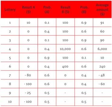
The lotteries used in this study are based on Rieger et.al (2011), as presented in Table 2. Risk preferences are calculated in the area of gains in the irst six lotteries by asking participants about their propensity to pay for these lotteries. The lotteries have binary results in Brazilian reals (R$) associated with the probability of each result’s occurrence. The lotteries were structured by combining diferent levels of results (R$ 10, R$ 100, R$ 400, R$ 10,000) with diferent levels of probabilities (0.1, 0.4, 0.5, 0.6 and 0.9). To diferentiate the area of risk propensity from the area of risk aversion, attitude towards risk in the area of losses was measured in the case of two lotteries (7 and 8).

The third measure, after the subjects have priced the eight lotteries, calculates the loss aversion coeicient. It is based on lotteries 9 and 10 (mixed lotteries) and asks the minimum amount of R$ thatthe participant would accept to participate in a bet with a 50% chance of losing a certainamount.

Table 2.

Prospects used in the study

Lottery Result A ($)

Prob. (A)

Result B ($)

Prob. (B)

Average amount

($)

1 10 0.1 100 0.9 91

2 0 0.4 100 0.6 60

3 0 0.1 100 0.9 90

4 0 0.4 10,000 0.6 6,000

5 0 0.9 100 0.1 10

6 0 0.4 400 0.6 240

7 - 80 0.6 0 0.4 - 48

8 - 100 0.6 0 0.4 - 60

9 - 25 0.5 - 0.5

-10 - 100 0.5 - 0.5

-Source: Rieger et al. (2011).

respondent’s lack of understanding, or their haste in completing the questionnaire survey.

a. If the amount given in the response for lottery 1 is less than or equal to R$ 10 or if it is more than or equal to R$ 100;

b. If the amount for lottery 3 is greater than the amount for lottery 1;

c. If the amounts for lotteries 2 or 5 are greater than R$ 100;

d. If the amount for lottery 7 is equal to or greater than R$ 80;

e. If the amount for lottery 8 is equal to or greater than R$ 100;

f. If the amount for lottery 7 is greater than the amount for lottery 8;

g. If the amount for lottery 9 is greater than R$ 500 and if the amount for lottery 10 is greater than R$ 2,000;

h. If the amount for lottery 9 is less than R$ 5 and the amount for lottery 10 is less than R$ 20;

i. If the amount for lottery 2 is R$ 100, if the amount for lottery 5 is R$ 100, and if the amount for lottery 6 is R$ 400.

Regarding the replication of lotteries used in Rieger et.al. (2011), some studies suggest that the values should be converted into local currency using each country’s purchasing power parity

(Harrison, Humphrey, & Verschoor, 2010, Rieger & Bui, 2011). However, it should be highlighted that these studies include a comparison between countries, which is not the case in this study. Considering that the average nominal Brazilian household income was R$ 1,052.00 in 2014 (IBGE, 2014), the monetary values of the lotteries seem to be quite realistic given the purpose of our analysis.

Estimation of parameters

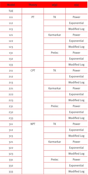
This study will be based on the three theories deined respectively in eqs. (6), (7) and (9) (prospect theory-PT; cumulative prospect

theory-CPT; normalized prospect theory-NPT), three value functions (power, exponential, and modiied logarithmic), and three weighting functions (Tversky-Kahneman-TK; Karmarkar; and Prelec), generating 27 models that are exhibited in Table 3. The utility fuuction, deined in eq. (1), will also be considered.

Table 3.

Models used

Model Theory w(p) v(x)

TUE

111 PT TK Power

112 Exponential

113 Modiied Log

121 Karmarkar Power

122 Exponential

123 Modiied Log

131 Prelec Power

132 Exponential

133 Modiied Log

211 CPT TK Power

212 Exponential

213 Modiied Log

221 Karmarkar Power

222 Exponential

223 Modiied Log

231 Prelec Power

232 Exponential

233 Modiied Log

311 NPT TK Power

312 Exponential

313 Modiied Log

321 Karmarkar Power

322 Exponential

323 Modiied Log

331 Prelec Power

332 Exponential

333 Modiied Log

Notes: For simpliication purposes, the following abbreviations were adopted throughout the text, in addition to those used in the table: Karmarkar: KAR; Prelec: PRC; Power: PWR; Exponential: EXP; Modiied Log: LOG.

In line with Bui (2009), this study uses the grid search methodology, which is explained below, to estimate all weighting and value function parameters, in order to minimize the sum of errors. Parameters are estimated for each individual and the error function is deined as the sum of the diferences between the certainty equivalent (CE) and the responses for all ten lotteries.

Each response should represent the individual’s CE to each of the ten prospects presented, as these responses represent the amount he/she has indicated for which they are indiferent in participating in the lottery or not. However, for each combination of α, β and δ, there is a fair CE amount, which in the case of optimal choice should be the same as the one in the individual’s response. The diference between the fair value of the CE for a prospect and the individual’s response to prospect i of the questionnaire is the itting error. The optimization process seeks to obtain the best combination of parameters α, β, δ and λ that exhibits the smallest sum of adjustment errors of the ten prospects.

To undertake this estimation, the study developed a Delphi algorithm, based on Bui (2009) to perform the grid optimization. Grid optimization uses nested loops with pre-determined value leaps to estimate the parameters. Once an optimal value is obtained, the result is reined, using smaller leaps consecutively around the optimal value found in the previous step. In this study, the parameters ranged from 0 to 1 in steps of 0.001. Mathematically the estimation process can be deined in the following way: in eqs. (6), (7) and (9), PT, CPT, and NPT were deined for a lottery with x_i results, each with probability p_i.

For this study, in which there are ten lotteries (Table 1) each with 2 results (A_i and B_i), the valueof each lottery prospect is deined as follows in eqs. (15), (16) and (17).

( ) ( )

(

) ( ),

PT

=

w p v B

+

w

1

-

p v A

( ) ( )

(

( )) ( ),

CPT

=

w p v B

+

1

-

w p

v A

( )

(

)

,

NPT

w p

w

p

PT

1

i

i i

i

=

+

-

where p_iis the probability of result B occurring in lottery i.

Grid search optimization methodology consists of inding the optimal combination of α, β and γ parameters that minimizes the error function, deined in eq. (18).

(

)

,

max

Error

A

B

CE

x

L

i i

i i

L 1

10

;

;;

;

;

;

=

|

-(

)

,

L

=

"

1 2

, ,

f

10

,

,

(18)

where value x_i is deined as each individual’s response to the data, which is the propensity to pay if x_i≥ 0, and the propensity to accept (negative value of the propensity to pay) if x_i< 0. This method is summarized in eq. (19).

( , , )

( , , )

min

optimal

a b c

=

a b c

|

(

)

,

, ,

,

max

A

B

CE

x

L

1 2

10

i i

i i

1

_;

_;;

_;

f

;

-

;

=

"

,

(19)

CE_i is deined for each lottery as the inverse of the value function in the calculation result for the prospect (Yi) for PT, CPT and NPT, as deined in eq. (20).

( )

CE

v

Y

1

=

-(20)

Table 4.

Calculation of the risk aversion parameter (λ)

m= + b

a b a ; E Exponential e e e e 1 1 2 1 1 1 A ax A ax 10 10 9 9 m -= -- ₊ b b -: D Modiied Log ( ) ( ) ( ) ( ) ln ln ln ln A ax A ax 2 1 1 1 1 1 9 9 10 10 m b_a

b b

= _-+ + _-+

a a

b l_{< F}

CPT Power ( ( . )) ( . ) ( ( . )) ( . ) w A w x w A w x

1 0 5

0 5 2

1

1 0 5

0 5 10 10 9 9 ; ; ; ; m

-= _- + b

a b a < F Exponential ( ( . ))( )) ( . )( ) ( ( . ))( )) ( . )( ) w e w e w e w e 2 1

1 0 5 1

0 5 1

1 0 5 1

0 5 1

A ax A ax 10 9 9 10 m= - - + -b b -< F Modiied Log ( ( . )( ( )) ( . )( ( )) ( ( . ))( ( )) ( . )( ( )) ln ln ln ln w A w x w A w x 2 1

1 0 5 1

0 5 1

1 0 5 1

0 5 1

9 9

10 10 m _ab

b a

b a

= b l< _- +_- + _- + _- F

Source: Adapted from Bui (2009).

In addition to the 27 combinations of value and weighting functions of the 3 variants of prospect theory, it is also important to assess the robustness of the EUT relative to prospect theory.

Given a prospect [(B, p; A, (1-p)], replacing u(x) in eq. (3) by eq. (1), we obtain the expected utility of this lottery as deined in eq. (21).

( , , )

(

)

(

)(

) ,

EU A B w

1

p B

w

1

1

p A

w

d

d

=

+

+

-

+

where w is deined as initial wealth.

Meanwhile, the CE is deined in eq. (22) below.

( , , )

( , , )

A B w

(

)

CE A B w

u

EU

w

EU

w

1

_d

=

6

@

-

=

-

The EUT optimization process is performed employing the same methodology used in prospect theory. The aim is to estimate the optimal value of δ that minimizes the error function.

( )

( )

(

)

,

, ,

,

( , , )

min

max

optimal

A

B

CE

x

L

s

A B w

1 2

10

i i i i i l 1 10

f

;

;;

;

;

;

d

=

d

-

=

=

"

,

Simultaneously, the level of initial wealth (w) is considered as the best value that minimizes the error function for a given value of δ. The limitation of this study relates to the size of the sample (75 respondents), which prevents us from generalizing its results to the entire Brazilian population. Additionally, as mentioned above, the sample is only partially representative of the general Brazilian population. However, the sample is justiied, because the aim of this study was to analyze the adequacy of behavioral models given the reality of Brazil. We consider this study to be an exploratory one given the lack of studies in this area to date.

RESULTS

Analysis of the Models

For each theory/weighting/value combination, we found the results that exhibited the fewest errors, as well as all the results within a certain percentage tolerance. The calibration of the tolerance percentage is an input of the model, and is based on the observed standard deviation to retain only those results that are statistically similar to the minimum error as optimal results.

In the results presented, we used a 30% tolerance percentage. To illustrate this concept, for example, if in the case of an observation using a NPT/KAR/LOG combination, the minimum error resulting from the optimization process was 0.3, all combinations that exhibited errors up to 30% above 0.3 (i.e., 0.39), were considered equally optimal. Table 5 shows the average, median and standard deviation of the risk aversion coeicient.

Table 5.

Risk aversion coeicient

Average Median Standard deviation Error

0.55 0.54 0.22 4.89

The δ coeicient result of 0.55 is in line with the literature

(Wakker, 2008, Palacios-Huerta & Serrano, 2006) and indicates relatively strong risk aversion (Holt & Laury, 2002). The results are similar to other studies such as Gonzalez and Wu (1999) (δ = 0.52), Tanaka, Camerer, and Nguyen (2010) (δ = 0.48) and Liu

(2012) (δ = 0.44).

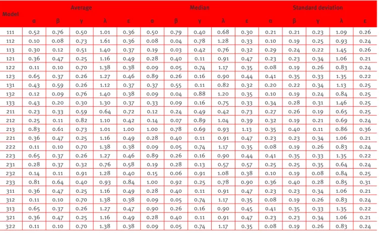
Table 6 shows the average, median and standard deviation of the α, β, γ and λ parameters of all models analyzed in this study, as listed in Table 2, in addition to each model’s associated error.

Table 6.

Details of the average, median and standard deviation

Model

Average Median Standard deviation

α β γ λ ε α β γ λ ε α β γ λ ε

111 0.52 0.76 0.50 1.01 0.36 0.50 0.79 0.40 0.68 0.30 0.21 0.21 0.23 1.09 0.26 112 0.10 0.08 0.73 1.61 0.36 0.08 0.04 0.78 1.28 0.33 0.10 0.19 0.25 0.93 0.24 113 0.30 0.12 0.51 1.40 0.37 0.19 0.03 0.42 0.76 0.32 0.29 0.24 0.22 1.45 0.26 121 0.36 0.47 0.25 1.16 0.49 0.28 0.40 0.11 0.91 0.47 0.23 0.23 0.34 1.06 0.21 122 0.11 0.10 0.70 1.38 0.38 0.09 0.05 0.74 1.17 0.35 0.08 0.19 0.26 0.83 0.24 123 0.65 0.37 0.26 1.27 0.46 0.89 0.26 0.16 0.90 0.44 0.41 0.35 0.33 1.35 0.22 131 0.43 0.59 0.26 1.12 0.37 0.37 0.55 0.11 0.82 0.32 0.20 0.22 0.34 1.13 0.25 132 0.12 0.09 0.76 1.40 0.38 0.09 0.04 0.88 1.20 0.35 0.10 0.19 0.24 0.84 0.25 133 0.43 0.20 0.30 1.30 0.37 0.33 0.09 0.16 0.75 0.33 0.34 0.28 0.31 1.46 0.25 211 0.23 0.33 0.59 0.64 0.72 0.12 0.24 0.49 0.42 0.73 0.27 0.26 0.19 0.65 0.25 212 0.25 0.11 0.82 1.10 0.42 0.14 0.07 0.89 1.04 0.39 0.32 0.19 0.21 0.69 0.24 213 0.83 0.61 0.73 1.01 1.00 1.00 0.78 0.69 0.93 1.13 0.35 0.40 0.11 0.86 0.36 221 0.36 0.47 0.25 1.16 0.49 0.28 0.40 0.11 0.91 0.47 0.23 0.23 0.34 1.06 0.21 222 0.11 0.10 0.70 1.38 0.38 0.09 0.05 0.74 1.17 0.35 0.08 0.19 0.26 0.83 0.24 223 0.65 0.37 0.26 1.27 0.46 0.89 0.26 0.16 0.90 0.44 0.41 0.35 0.33 1.35 0.22 231 0.28 0.37 0.32 0.76 0.58 0.19 0.28 0.13 0.57 0.57 0.25 0.25 0.35 0.64 0.24 232 0.14 0.11 0.91 1.28 0.40 0.15 0.06 0.91 1.08 0.38 0.10 0.19 0.08 0.84 0.25 233 0.81 0.64 0.40 0.93 0.84 1.00 0.92 0.25 0.78 0.90 0.36 0.40 0.28 0.85 0.31 311 0.36 0.47 0.25 1.16 0.49 0.28 0.40 0.11 0.91 0.47 0.23 0.23 0.34 1.06 0.21 312 0.11 0.10 0.70 1.38 0.38 0.09 0.05 0.74 1.17 0.35 0.08 0.19 0.26 0.83 0.24 313 0.65 0.37 0.26 1.27 0.47 0.90 0.26 0.16 0.90 0.45 0.41 0.35 0.33 1.35 0.22 321 0.36 0.47 0.25 1.16 0.49 0.28 0.40 0.11 0.91 0.47 0.23 0.23 0.34 1.06 0.21 322 0.11 0.10 0.70 1.38 0.38 0.09 0.05 0.74 1.17 0.35 0.08 0.19 0.26 0.83 0.24

Model

Average Median Standard deviation

α β γ λ ε α β γ λ ε α β γ λ ε

323 0.65 0.37 0.26 1.27 0.46 0.89 0.26 0.16 0.90 0.44 0.41 0.35 0.33 1.35 0.22 331 0.36 0.47 0.24 1.15 0.49 0.28 0.40 0.08 0.93 0.47 0.23 0.23 0.35 1.05 0.21 332 0.10 0.10 0.65 1.38 0.38 0.09 0.05 0.69 1.16 0.35 0.06 0.19 0.27 0.83 0.25 333 0.65 0.37 0.24 1.28 0.46 0.89 0.26 0.12 0.91 0.44 0.41 0.35 0.33 1.36 0.22

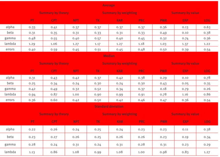
Table 7 presents the consolidation of Table 6, considering the average, median and standard deviation resulting from optimization. Analyzing both tables, we draw the following conclusions: starting with the average of parameters α and β, which measures the slope of the utility function of money in the gains and losses areas respectively, we observe that, in all models, α < 1 and β < 1. This is expected, given that the psychological concept of diminishing sensitivity implies that α < 1 and β <1 (i.e., the further individuals are from the point of reference, the more sensitive they are to change (Booj, Van Praag &Van De Kuilen., 2010)). In addition, the results show a typical S-shaped value function (i.e., concave in the region of gains and convex in the region of losses). However, S-shaped value function difer according to each model.

Table 7.

Consolidated average, median and standard deviation data by theory, weighting and value

Average

Summary by theory Summary by weighting Summary by value

PT CPT NPT TK KAR PRC PWR EXP LOG

alpha 0.33 0.41 0.37 0.37 0.37 0.37 0.36 0.13 0.63

beta 0.31 0.35 0.31 0.33 0.31 0.33 0.49 0.10 0.38

gamma 0.48 0.55 0.40 0.57 0.40 0.45 0.32 0.74 0.36

lambda 1.29 1.06 1.27 1.17 1.27 1.18 1.03 1.37 1.22

errors 0.40 0.59 0.45 0.51 0.45 0.48 0.50 0.39 0.54

Median

Summary by theory Summary by weighting Summary by value

PT CPT NPT TK KAR PRC PWR EXP LOG

alpha 0.31 0.43 0.42 0.37 0.42 0.38 0.29 0.10 0.78

beta 0.25 0.34 0.24 0.30 0.24 0.30 0.43 0.05 0.35

gamma 0.42 0.49 0.32 0.52 0.34 0.37 0.18 0.79 0.26

lambda 0.94 0.87 1.00 0.90 0.99 0.91 0.78 1.16 0.86

errors 0.36 0.60 0.42 0.50 0.42 0.46 0.47 0.36 0.54

Standard deviation

Summary by theory Summary by weighting Summary by value

PT CPT NPT TK KAR PRC PWR EXP LOG

alpha 0.22 0.26 0.24 0.25 0.24 0.23 0.23 0.11 0.38

beta 0.23 0.27 0.26 0.25 0.26 0.26 0.23 0.19 0.34

gamma 0.28 0.24 0.31 0.24 0.31 0.28 0.31 0.23 0.29

lambda 1.13 0.86 1.08 0.99 1.08 1.00 0.98 0.83 1.27

In general, models based on the exponential function exhibited a steeper S-shaped function than power and modiied log functions, while the modiied log function had a less steep curve than the power function. Another important characteristic is that β > α in both models 111 and 131, which is in line with results of other studies that demonstrate that losses are assessed in a more

linear fashion than gains (Booj et al., 2010). This suggests that people are less sensitive to additional gains than to additional losses (Booj et al., 2010).

The mean of the probability distortion parameter γ is less than 1 in all the models, showing that there is a clear distortion of probabilities in the subjects studied. In addition, there is a clear loss aversion given that the mean of the loss aversion parameter is greater than 1 in all models.

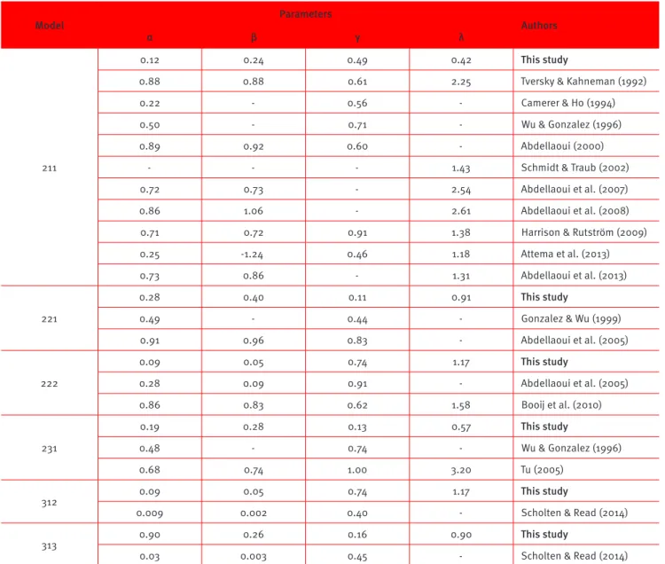
The values found in this study for parameters α and β in the individual models are, in the majority of cases, lower than the values found in studies performed in developed countries (Table 8). The same holds for the probability distortion (γ) and the risk aversion parameter (λ).

Table 8.

Summary of studies performed in developed countries

Model

Parameters

Authors

α β γ λ

211

0.12 0.24 0.49 0.42 This study

0.88 0.88 0.61 2.25 Tversky & Kahneman (1992)

0.22 - 0.56 - Camerer & Ho (1994)

0.50 - 0.71 - Wu & Gonzalez (1996)

0.89 0.92 0.60 - Abdellaoui (2000)

- - - 1.43 Schmidt & Traub (2002)

0.72 0.73 - 2.54 Abdellaoui et al. (2007)

0.86 1.06 - 2.61 Abdellaoui et al. (2008)

0.71 0.72 0.91 1.38 Harrison & Rutström (2009)

0.25 -1.24 0.46 1.18 Attema et al. (2013)

0.73 0.86 - 1.31 Abdellaoui et al. (2013)

221

0.28 0.40 0.11 0.91 This study

0.49 - 0.44 - Gonzalez & Wu (1999)

0.91 0.96 0.83 - Abdellaoui et al. (2005)

222

0.09 0.05 0.74 1.17 This study

0.28 0.09 0.91 - Abdellaoui et al. (2005)

0.86 0.83 0.62 1.58 Booj et al. (2010)

231

0.19 0.28 0.13 0.57 This study

0.48 - 0.74 - Wu & Gonzalez (1996)

0.68 0.74 1.00 3.20 Tu (2005)

312 0.09 0.05 0.74 1.17 This study

0.009 0.002 0.40 - Scholten & Read (2014)

313

0.90 0.26 0.16 0.90 This study

0.03 0.003 0.45 - Scholten & Read (2014)

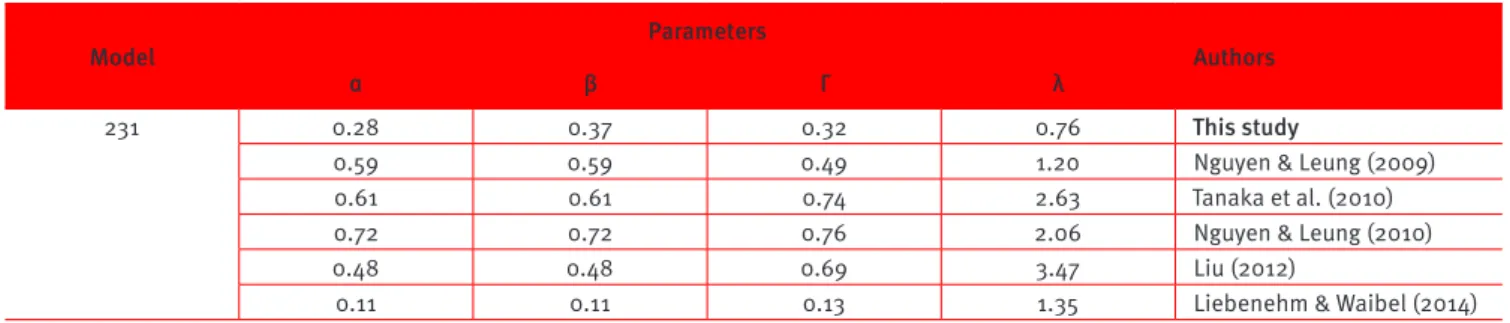
Table 9.

Summary of studies performed in developing countries

Model

Parameters

Authors

α β Γ λ

231 0.28 0.37 0.32 0.76 This study

0.59 0.59 0.49 1.20 Nguyen & Leung (2009)

0.61 0.61 0.74 2.63 Tanaka et al. (2010)

0.72 0.72 0.76 2.06 Nguyen & Leung (2010)

0.48 0.48 0.69 3.47 Liu (2012)

0.11 0.11 0.13 1.35 Liebenehm & Waibel (2014)

As expected, the results of this study difer in part from those found in other studies. Booj et al. (2010) surveyed several studies and found a large variability in estimated parameters. According to the authors, a possible explanation is the hypothetical bias, which means people do not behave in a realistic manner when the stakes are not real (and are just for ‘play’). Some studies have tried to circumvent this by ofering real inancial incentives. Another explanation is related to the econometric methodology, as some studies use a non-parametric approach, while others use a parametric methodology. Finally,

there are explanations of a cultural nature as explained in Rieger et al. (2017).

The next step is to analyze the list of optimal results for each combination. The results are presented in descending order of the combination of optimal results. Table 10 shows the number of optimal models in each theory combination in the sample of 75 individuals. For example, for 54 individuals models 111 and 131 have the best optimization results. This represents 8.3% of the distribution of all theory combinations. We note that exponential functions dominate in the best optimization results as they are prevalent in the ten best results.

Table 10.

Optimal results by model

Model Description % Quantity PT CPT NPT TK KAR PRC PWR EXP LOG

111 pt-tk-pwr 8.3% 54 54     54     54    

131 pt-prc-pwr 8.3% 54 54         54 54    

133 pt-prc-log 7.3% 48 48         48     48

112 pt-tk-exp 6.6% 43 43     43       43  

113 pt-tk-log 6.3% 41 41     41         41

132 pt-prc-exp 5.5% 36 36         36   36  

332 npt-prc-exp 5.2% 34     34     34   34  

122 pt-kar-exp 4.9% 32 32       32     32  

222 cpt-kar-exp 4.9% 32   32     32     32  

312 npt-tk-exp 4.9% 32     32 32       32  

322 npt-kar-exp 4.9% 32     32   32     32  

232 cpt-prc-exp 4.3% 28   28       28   28  

212 cpt-tk-exp 2.9% 19   19   19       19  

123 pt-kar-log 2.6% 17 17       17       17

223 cpt-kar-log 2.6% 17   17     17       17

313 npt-tk-log 2.6% 17     17 17         17

323 npt-kar-log 2.6% 17     17   17       17

333 npt-prc-log 2.4% 16     16     16     16

331 npt-prc-pwr 1.8% 12     12     12 12    

121 pt-kar-pwr 1.8% 12 12       12   12    

221 cpt-kar-pwr 1.8% 12   12     12   12    

321 npt-kar-pwr 1.8% 12     12   12   12    

311 npt-tk-pwr 1.8% 12     12 12     12    

231 cpt-prc-pwr 1.5% 10   10       10 10    

211 cpt-tk-pwr 1.4% 9   9   9     9    

213 cpt-tk-log 0.5% 3   3   3         3

Regarding the data consolidation shown in Table 11, we note that, in terms of theory, PT exhibits the best performance with 51.53%, while CPT exhibits the worst with 20.34%. When analyzed accordingto weighting, PRC registers the best performance with 36.85%, immediately followed by TK with 35.17%, and KAR recording the worst performance. In the case of value functions, the exponential function exhibited the best result with 44.04% and the worst was the power function.

Table 11.

Consolidated optimization data by theory, weighting/weight and value

Summary by theory Summary by weighting Summary by value

PT CPT NPT TK KAR PRC PWR EXP LOG

337 133 184 230 183 241 187 288 179

51.53% 20.34% 28.13% 35.17% 27.98% 36.85% 28.59% 44.04% 27.37%

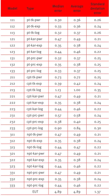
Table 12.

Median, average and standard deviation

estimation error by theory and weighting

Model Type Median error

Average error

Standard deviation error

111 pt-tk-pwr 0.30 0.36 0.26

112 pt-tk-exp 0.33 0.36 0.24

113 pt-tk-log 0.32 0.37 0.26

121 pt-kar-pwr 0.47 0.49 0.21

122 pt-kar-exp 0.35 0.38 0.24

123 pt-kar-log 0.44 0.46 0.22

131 pt-prc-pwr 0.32 0.37 0.25

132 pt-prc-exp 0.35 0.38 0.25

133 pt-prc-log 0.33 0.37 0.25

211 cpt-tk-pwr 0.73 0.72 0.25

212 cpt-tk-exp 0.39 0.42 0.24

213 cpt-tk-log 1.13 1.00 0.35

221 cpt-kar-pwr 0.47 0.49 0.21

222 cpt-kar-exp 0.35 0.38 0.24

223 cpt-kar-log 0.44 0.46 0.22

231 cpt-prc-pwr 0.57 0.58 0.24

232 cpt-prc-exp 0.38 0.40 0.25

233 cpt-prc-log 0.90 0.84 0.30

311 npt-tk-pwr 0.47 0.49 0.21

312 npt-tk-exp 0.35 0.38 0.24

313 npt-tk-log 0.44 0.47 0.22

321 npt-kar-pwr 0.47 0.49 0.21

322 npt-kar-exp 0.35 0.38 0.24

323 npt-kar-log 0.44 0.46 0.22

331 npt-prc-pwr 0.47 0.49 0.21

332 npt-prc-exp 0.35 0.38 0.24

333 npt-prc-log 0.44 0.46 0.22

EUT 4.89 4.89 1.37

Table 12 presents the median, average and standard deviation errors according to theory and weighting. We observe the superiority of behavioral models relative to EUT. In addition, models based on prospect theory with weighting functions TK and Prelec, value functions power and modiied log performed better than the others. This is in line with the literature (Stott, 2006 and Bui, 2009) and, in our case, it shows the superior performance of the function proposed in this study, the modiied log.

The superior performance of the modiied log function is that it its well in the reality of individual decision making (i.e., it remains concave to high values of “x”, even for α and β values close to one). For alpha and beta values above 1, the function ceases to be concave in the gain region and convex in the loss region. Also, the function is not valid for negative values of α and β. The valid values of α and β for the modiied log function are in the interval [0,1], with good sensitivity to increments of 0.01. A basic diference of this function and the power function is that the power function tends to be linear for all ranges of values when α and β approach 1, which does not it well with the observed data.

CONCLUSIONS

This study analyzed risk preferences in Brazil based on prospect theory. To achieve these estimations were performed of the risk aversion parameter of the Expected Utility Theory for a selected sample, and of the value and probability function parameters, assuming various functional forms, and a new value function – the modiied log - was suggested.

diferences are presented in the literature, such as in studies related to econometric methodology and the hypothetical bias. Recent studies has also added cultural inluence as a possible explanatory variable.

As expected, the study found that behavioral models were superior to the EUT. In addition, models based on the prospect theory, TK and Prelec weighting functions and the power value function performed better than others, thus conirming prior expectations. Finally, the modiied log function proposed in the study it the data well, and can thus be used in future studies in Brazil. This can be due to speciic characteristics of this function, which make it robust to possible outliers.

There are important applications of the results of studies such as this one, especially with regards to the allocation of resources. For banks and brokerage irms, it is important to know the level of risk aversion and deviations from behavior considered rational when ofering investment options. Often, the questionnaires used by these agents fail to determine the exact risk proile of the investors, and may lead to a misallocation of investor resources within an expected risk-return context.

ACKNOWLEDGMENT

This work was carried out with the support of Conselho Nacional de Desenvolvimento Cientíico e Tecnológico (National Council for Scientiic and Technological Development - CNPq), number 305842/2013-7.

REFERENCES

Abdellaoui, M. (2000). Parameter-free elicitation of utility and

probability weighting functions. Management Science, 46(11),

1497-1512.

Abdellaoui, M., Bleichrodt, H., & L’Haridon, O. (2008). A tractable method to measure utility and loss aversion under prospect theory.

Journal of Risk and Uncertainty, 36(3), 245-266. doi:10.1007/s11166-008-9039-8

Abdellaoui, M., Bleichrodt, H., & L’Haridon, O. (2013). Sign-dependence

in intertemporal choice.Journal of Risk and Uncertainty, 47(3),

225-253. doi:10.1007/s11166-013-9181-9

Abdellaoui, M., Bleichrodt, H., & Paraschiv, C. (2007). Loss aversion

under prospect theory: A parameter-free measurement.Management

Science, 53(10), 1659-1674.

Abdellaoui, M., Vossmann, F., & Weber, M. (2005). Choice-based elicitation and decomposition of decision weights for gains and

losses under uncertainty.Management Science,51(9), 1384-1399.

Allais, M. (1953). Le comportement de l’homme rationnel devant le

risque: Critique des postulats et axiomes de l’ecole americaine.

Econometrica, 21(4), 503-546. doi:10.2307/1907921

Attema, A. E., Brouwer, W. B. F., & L’Haridon, O. (2013). Prospect theory

in the health domain: A quantitative assessment.Journal of Health

Economics, 32(6), 1057-1065. doi:10.1016/j.jhealeco.2013.08.006

Barberis, N., & Huang, M. (2008). Stocks as lotteries: The implications

of probability weighting for security prices. American Economic

Review, 98(5), 2066-2100.

Barberis, N., Huang, M., & Santos, T. (2001). Prospect theory and

asset prices. The Quarterly Journal of Economics, 116(1), 1-53.

doi:10.1162/003355301556310

Bernoulli, D. (1954). Exposition of a new theory on the measurement of

risk. Econometrica, 22(1), 23-36. doi:10.2307/1909829

Booj, A., van Praag, B., & van de Kuilen, G. (2010). A parametric analysis

of prospect theory’s functionals for the general population. Theory

and Decision, 68(1-2), 115-148. doi:10.1007/s11238-009-9144-4

Bui, T. (2009). Prospect Theory and Functional Choice. A Dissertation Submitted to the Graduate School in Partial Fulillment of the Requirements for the Degree Erasmus Mundus Master: Models and Methods of Quantitative Economics (QEM), Bielefeld University and The University of Paris 1 Panthéon-Sorbonne.

Camerer, C. F., & Ho, T.-H. (1994). Violations of the betweenness axiom

and nonlinearity in probability.Journal of Risk and Uncertainty, 8(2),

167-196. doi:10.1007/BF01065371

Ellsberg, D. (1961). Risk, ambiguity, and the savage axioms. The Quarterly Journal of Economics,75(4), 643-669.

Fishburn, P. C., & Kochenberger, G. A. (1979). Two-piece Von

Neumann-Morgenstern utility functions. Decision Sciences, 10(4), 503-518.

doi:10.1111/j.1540-5915.1979.tb00043.x

Gerber, H. U., & Pafum, G. (1998). Utility functions: From risk theory to

inance. North American Actuarial Journal, 2(3), 92-94. doi:10.1080/

10920277.1998.10595731

Goldstein, W. M., & Einhorn, H. J. (1987). Expression theory and the preference reversal phenomena. Psychological Review, 94(2), 236-254. doi:10.1037/0033-295X.94.2.236

Gomes, F. J. (2005). Portfolio choice and trading volume with

loss‐averse investors. The Journal of Business, 78(2), 675-706.

doi:10.1086/427643

Gonzalez, R., & Wu, G. (1999). On the shape of the probability weighting

function. Cognitive Psychology, 38(1), 129-166. doi:10.1006/

cogp.1998.0710

Harrison, G., & Rutström, E. (2009). Expected utility theory and prospect

theory: One wedding and a decent funeral. Experimental Economics,

12(2), 133-158. doi:10.1007/s10683-008-9203-7

Harrison, G. W., Humphrey, S. J., & Verschoor, A. (2010). Choice under

uncertainty: Evidence from Ethiopia, India and Uganda.The Economic

Journal, 120(543), 80-104. doi:10.1111/j.1468-0297.2009.02303.x

Holt, C. A., & Laury, S. K. (2002). Risk aversion and incentive efects.

American Economic Review, 92(5), 1644-1655.

Instituto Brasileiro de Geograia e Estatística(IBGE). (2014). Pesquisa Nacional por Amostra de Domicílios (Pnad) Contínua. Brasilia, DF.

Kahneman, D., & Tversky, A. (1979). Prospect theory: An

analysis of decision under risk. Econometrica, 47(2), 263-292.

Karmarkar, U. S. (1978). Subjectively weighted utility: A descriptive

extension of the expected utility model.Organizational Behavior and

Human Performance, 21(1), 61-72. doi:10.1016/0030-5073(78)90039-9

Karmarkar, U. S.. (1979). Subjectively weighted utility and the Allais

Paradox.Organizational Behavior and Human Performance,24(1),

67-72. doi:10.1016/0030-5073(79)90016-3

Köbberling, V., & Wakker, P. P. (2005). An index of loss aversion.Journal of Economic Theory,122(1), 119-131. doi:10.1016/j.jet.2004.03.009

Liebenehm, S., & Waibel, H. (2014). Simultaneous estimation of risk and time preferences among small-scale cattle farmers in West

Africa.American Journal of Agricultural Economics, 96(5), 1420-1438.

doi:10.1093/ajae/aau056

Liu, E. M. (2012). Time to change what to sow: Risk Preferences and

technology adoption decisions of cotton farmers in China.Review of

Economics and Statistics, 95(4), 1386-1403. doi:10.1162/REST_a_00295

Machina, M. J. (2008). Non-expected utility theory. In S. N. Durlauf & L. E. Blume (Eds.), The New Palgrave Dictionary of Economics, 2nd _Edition.

London, UK: Palgrave Macmillan.

Markowitz, H. (1952). Portfolio selection. The Journal of Finance, 7(1), 77-91. doi:10.1111/j.1540-6261.1952.tb01525.x

Nguyen, Q., & Leung, P. (2009). Do Fishermen have Diferent Attitudes Toward Risk? An Application of Prospect Theory to the Study of

Vietnamese Fishermen. Journal of Agricultural and Resource

Economics, 34(3), 518-538.

Nguyen, Q., & Leung, P. (2010). How nurture can shape preferences: An experimental study on risk preferences of Vietnamese ishers.

Environment and Development Economics, 15(5), 609-631. doi:10.1017/S1355770X10000203

Palacios-Huerta, I., & Serrano, R. (2006). Rejecting small gambles under

expected utility.Economics Letters, 91(2), 250-259. doi:10.1016/j.

econlet.2005.09.017

Prelec, D. (1998). The probability weighting function. Econometrica, 66(3), 497-527. doi:10.2307/2998573

Rieger, M. O., Wang, M., & Hens, T. (2011). Prospect theory around the world (October 31, 2011). NHH Dept. of Finance & Management Science Discussion Paper No. 2011/19.

Rieger, M., & Wang, M. (2008). Prospect theory for continuous

distributions. Journal of Risk and Uncertainty, 36(1), 83-102.

doi:10.1007/s11166-007-9029-2

Rieger, M. O., & Bui, T. (2011). Too risk-averse for prospect theory?

Modern Economy, 2(4), 691-670. doi:10.4236/me.2011.24077

Rieger, M. O., Wang, M., & Hens, T. (2017). Estimating cumulative

prospect theory parameters from an international survey.Theory and

Decision, 82(4), 567-596. doi:10.1007/s11238-016-9582-8

Schmidt, U., & Traub, S. (2002). An experimental test of loss

aversion. Journal of Risk and Uncertainty, 25(3), 233-249.

doi:10.1023/A:1020923921649

Scholten, M., & Read, D. (2014). Prospect theory and the “forgotten”

fourfold pattern of risk preferences. Journal of Risk and Uncertainty,

48(1), 67-83. doi:10.1007/s11166-014-9183-2

Stott, H. P. (2006). Cumulative prospect theory’s functional menagerie.

Journal of Risk and Uncertainty, 32(2), 101-130. doi:10.1007/s11166-006-8289-6

Tanaka, T., Camerer, C. F., & Nguyen, Q. (2010). Risk and time preferences: Linking experimental and household survey data from

Vietnam.American Economic Review, 100(1), 557-571. doi:10.1257/

aer.100.1.557

Tu, Q. (2005). Empirical analysis of time preferences and risk aversion. Tilburg University: CentER, Center for Economic Research.

Tversky, A., & Kahneman, D. (1992). Advances in prospect theory:

Cumulative representation of uncertainty. Journal of Risk and

Uncertainty, 5(4), 297-323.

Tversky, A., & Wakker, P. (1995). Risk attitudes and decision weights.

Econometrica, 63(6), 1255-1280. doi:10.2307/2171769

von Neumann, J., & Morgenstern, O. (1944). Theory of Games and Economic Behavior. Princeton, USA: Princeton University Press.

Wakker, P. P. (2008). Explaining the characteristics of the power (CRRA)

utility family. Health Economics, 17(12), 1329-1344. doi:10.1002/

hec.1331

Wu, G., & Gonzalez, R. (1996). Curvature of the probability weighting

function.Management Science,42(12), 1676-1690.

Zeisberger, S., Vrecko, D., & Langer, T. (2012). Measuring the time

stability of Prospect Theory preferences.Theory and Decision, 72(3),