INSTITUTO SUPERIOR DE ECONOMIA E GEST ˜
AO
UNIVERSIDADE T´
ECNICA DE LISBOA
MASTER
FINANCE
MASTER THESIS
DISSERTATION
CUMULATIVE PROSPECT THEORY: A PARAMETRIC ANALYSIS OF
THE FUNCTIONAL FORMS AND APPLICATIONS
ANA TORRE DO VALLE DE ARRIAGA E CUNHA
ORIENTATION
RAQUEL M. GASPAR PEDRO RINO VIEIRA
Cumulative Prospect Theory: A parametric analysis of the
functional forms and applications
Ana Arriaga e Cunha
Abstract
This work presents an empirical study of the cumulative prospect theory using a Portuguese sample. We estimate the value function and the probability weighting function with positive and negative outcomes. The results confirm previous works that the value function is concave in the gain domain and almost linear in the loss domain. Our results also show an inverse S-shape for the probability weighting function in both loss and gain domain.
We also look into the relation of the coefficient from the already mentioned functions with some demographic variables. It was possible to conclude that males are more willing to take risks than females.
Abstract
Este trabalho apresenta um estudo emp´ırico sobre cumulative prospect theory atrav´es do estudo da fun¸c˜ao de utilidade e a fun¸c˜ao de probabilidade distorcida. Os resultados obtidos est˜ao de acordo com a literatura, que mostra que a fun¸c˜ao da utilidade ´e cˆoncava no dom´ınio dos ganhos, e quase linear no dom´ınio das perdas. ˜N˜ao s´o mostra que a fun¸c˜ao da probabilidade distorcida tem a forma de um “S” inverso tanto no dom´ınio dos ganhos como no dom´ınio das perdas. Tamb´em aborda o estudo de vari´aveis demogr´aficas relacionando-as com os coeficientes das fun¸c˜oes mencionadas anteriormente, concluindo assim que os homens est˜ao mais dispostos a correr riscos do que as mulheres.
Contents
1 Introduction 1
2 Literature Review 4
2.1 Theories . . . 4 2.2 Functional Forms . . . 8
3 Data & Methodology 13
3.1 Survey . . . 13 3.2 Methodology . . . 15
4 Results 18
4.1 Functional forms . . . 19 4.2 Demographic Model . . . 23
5 CPT Applications 27
5.1 CPT and DOSPERT-Scale . . . 27 5.2 CPT and Mean Variance Applications . . . 29 5.2.1 The Empirical PSD efficient frontier . . . 31
6 Conclusion and Further Research 33
References 35
A Appendix 38
List of Figures
2.1 Hypothetical curves of original prospect theory . . . 7
2.2 Hypothetical curves of cumulative prospect theory . . . 8
2.3 Variations of probability weighting functions . . . 11
4.1 Estimated functions of prospect theory . . . 22
5.1 The MV and PSD efficient frontiers . . . 30
5.2 The PSD efficient frontiers . . . 32
List of Tables
4.1 Sample statistics . . . 18
4.2 Certainty equivalent median . . . 19
4.3 Estimated coefficients: Probability weighting function . . . 19
4.4 Estimated coefficients: Value function . . . 21
4.5 Classification of respondents . . . 21
4.6 Estimated coefficients: Second approach . . . 23
4.7 Linear Regression for the Demographic Variables . . . 24
1.
Introduction
The expected utility theory is the most renown theory that describes the decision making process of an individual with regard to uncertain outcomes. However, after some empirical work, it has been demonstrated that this theory fails to correctly explain the risk preferences of an individual. Some theories of non-expected utility have been proposed to explain these prefer-ences, but the more prominent is the cumulative prospect theory by Tversky and Kahneman (1992).
This theory differs from the expected utility theory in four important aspects: (i) the prefer-ences are defined in terms of gains and losses instead of absolute wealth; (ii) decision makers are more sensitive to small winnings compared to big winnings; (iii) losses seem larger than gains and finally; (iv) people are more sensitive to extreme probabilities.
These discoveries of Tversky and Kahneman (1992) have had big impact on the value and weighting functions. As the expected utility theory has a utility function commonly represented as concave and a linear probability function, the cumulative prospect theory has an S-shape utility function that describes the conclusion (i), (ii) and (iii) and an inverse S-shape probability weighting function that explains the fourth conclusion.
The change of the utility theory has had a big impact with regards to the risk decision making process in a variety of disciplines, such as economics, finance and marketing. It is therefore of the utmost importance to better understand this new theory, with regards to issues like: the kind of human characteristics that can influence decisions, how it can be used, and how it is going to change the theories that used the expected utility theory? These are the kind of questions this work will aim to answer.
The calculation of the prospect theory coefficients is not a simple task, as it requires a lot of calculations and a complex survey that entails a lot of explanation and is not accessible to everyone. The third objective is to establish a bridge between the coefficient of loss aversion and the DOSPERT-scale. Weber et al. (2002) have proposed the DOSPERT (Domain Specific Risk Taking).
This scale has the objective of assessing the risk taking of an individual in five domains (finance, health, recreational, ethical and social). In this scale, each individual rates the likeli-hood of engaging in a specific activity considering the risk they are taking. Despite this scale measure five domains, we will just focus on the field of finance. The benefit of creating a link between this scale and prospect theory is the simplicity of applying this scale to an individual and obtaining the loss aversion coefficient, as the traditional method to obtain this coefficient requires a lot of calculations and assumptions. As said before, the first study of the DOSPERT scale was proposed by Weber et al. (2002) with an English scale, and after that, many papers were published with the translation of the same scale. In this case, since we are studying a Portuguese sample, we are more interested in using the Portuguese DOSPERT-scale proposed by Silva (2012).
The final objective of this work is to study the implication in financial markets of replacing the expected utility theory for the cumulative prospect theory. As we know there are a lot of theories that used the expected utility theory, however in this work we are more interested in studying the financial domain. As so, we will study the differences in the efficient frontier of the Portuguese market using cumulative prospect theory instead of the expected utility theory. With this new market information, individually and globally, financial institutions will be provided with much better information about their clients and what kind of products are more suitable to them.
If we try to group these four objectives into one, we could say we are attempting to make an implementation of the cumulative prospect theory over the expected utility theory in the chain of risky choice. Starting individually where we present the risks to a group of individuals, and end up with a global view of the financial markets.
2.
Literature Review
The expected utility theory is the most renown theory of risky decisions. However this theory has been discredited by several authors like Allais (1953) and Kahneman and Tversky (1979). This chapter will explore in great detail the development of prospect theory, from the beginning (Expected Utility Theory) to the most recent (Cumulative Prospect Theory). It will also describe in great detail the functional forms that are included in this last theory.
Making this study with a Portuguese sample is very helpful for the Portuguese financial institutions as, to the best of our knowledge, this study belongs to a series of studies that apply for the first time prospect theory to a Portuguese sample. These studies were develop by a research team composed by master and PhD. students.
2.1
Theories
As said at the beginning of this chapter, the expected utility theory (EUT) is the theory commonly used when an individual has to make a decision under risky conditions, where he is faced with finite outcomes each of which has a respective probability of occurring.
The EUT asserts that the individuals try to maximise their expected utility taking into account the probability of each outcome and their respective utility. Each person has a specific utility curve. For example, the impact a wealthy person receiving an additional 100AC in their
monthly income will differ from that of non wealthy person receiving the same amount. That is why to calculate the utility of a decision under risk we have to take into account the benefit to the person that has to choose. The decision maker chooses the option with the highest EU, which can be described as,
Nevertheless many empirical studies show that there are some “anomalies” in this theory. The biggest “anomaly” were presented by Allais (1953) and it is commonly known as the “Allais Paradox”. This author showed that people are more sensitive to differences in the probabilities near the extreme point (0% and 100%) than in the middle points (around 50%).
Another “anomaly” that the EUT can not take into account is the fourfold pattern of risk attitudes: “risk seeking for low-probability gains and high-probability losses, coupled with risk aversion for high-probability gains and low-probability losses”. This paradox, in particular risk seeking for low-probability gains and risk aversion for low-probability losses, may explain the attraction for gambling and insurance. Risk aversion for high-probability gains may contribute to the preference for certainty whereas risk seeking for high-probability losses is consistent with the common tendency to undertake risk to avoid facing sure losses.
Kahneman and Tversky (1979) developed the Prospect Theory (PT) which takes into account the Allais paradox and the fourfold pattern of risk attitudes. Levy (1992) summarised the most important aspects of this theory as follow:
1. People tend to think in terms of gains and losses instead of absolute wealth, therefore the choices made by a person are codified in terms of deviations of the reference point. The reference point can be seen as the status quo of an individual, i.e., the wealth that an individual has at the moment of the choice. Another type of reference point could be the aspiration level, in that case the gains and losses are measured by deviations from the aspiration level.
2. People react differently to gains and losses. Normally they are risk-averse in the domain of gains, and risk-seeking in the domain of losses. This has an impact in the value function shape, suggesting that in the domain of gains, the curve is concave and in the domain of losses the curve is convex. Kahneman and Tversky (1979) titled this phenomenon as the
reflection effect around the reference point. The reflection effect basically states that the sensitiveness close to the reference point is elevated and it decreases as the distance from the reference point increases, in both directions (losses and gains). This can only prevail if the utility function is not strictly concave or convex in all domain.
same absolute value”. Another phenomenon calledendowment effect is when people give more value to things they possess than to the equivalent but that they do not possess. 4. There is a nonlinear transformation of the probability scale, which has some consequences:
people overweight events with small probabilities and underweight events with higher probabilities, i.e., changes in extreme probabilities (0% and 100%) have greater impact then changes in the middle probabilities -certainty effect.
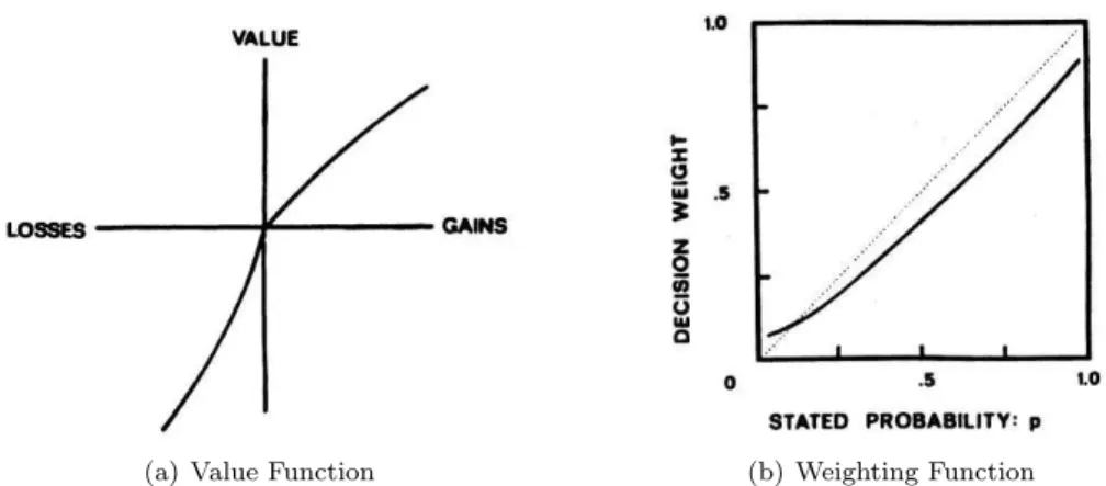
From this paper we can retrieve two important functions: the value function and the prob-ability weighting function. The value function is the surrogate of the utility function in the previous theory. This function is defined as deviations from the reference point, withv(0) = 0, instead of measuring absolute wealth. Generally it is concave for gains and convex for losses, having a S-shape form that implies a diminishing sensitivity as we move away from the reference point (reflection effect). Finally, it is steeper in the losses than in the gains (loss aversion and
endowment effect). Figure 2.1(a) is a representation of an hypothetical value function. The value function of a simple prospect that pays xAC with a probabilityp, otherwise nothing, is
given by:
V(x, p) =w(p)v(x) (2.2) where v(x) measures the subjective value of the consequence x. The function w(p) measures the impact of the probabilitypon the attractiveness of the prospect and is called probability weighting function. From now on this kind of prospect is described by (x, p; 0).
The probability weighting function “measures the impact of the probability of an event on the desirability of a prospect”. As showed in the equation 2.2 the value of the outcome is not weighted by the probability of this occurring, but by a decision weight w(p). This decision weight is the perception of the probability that a decision maker has towards a specific probability. By definition w(0) = 0 and w(1) = 1. This function is nonlinear due to the fact that individuals attribute more weight to events with small probabilities and less weight to the higher probabilities (certainty effect) and a possible representation of this curve is presented on figure 2.1(b)
(a) Value Function (b) Weighting Function
Figure 2.1: Hypothetical curves of original prospect theory
by Tversky and Kahneman (1992) when they proposed the cumulative prospect theory (CPT). The CPT instead of transforming each probability separately uses a separate cumulative distribution functions for gains and losses. That is, an outcomexis not weighted by its prob-ability but by the cumulative probprob-ability of obtaining an outcome at least as good asxif the outcome is positive, and at least as bad asxif the outcome is negative. With this improvement the CPT allows more than two nonzero outcomes and does not have the stochastic dominance violation problem. The CPT also allows different weighting functions for losses (w(p)−) and
gains (w(p)+).
The value function of a prospect described by (x, p;y, q) can be:
Mixed Prospect: V =w−(p)v(x) +w+(p)v(y) if x<0<y ;
Pure Gain Prospect: V = [w+(p+q)−w+(q)]v(x) +w+(q)v(y) if 0≤x<y ;
Pure Loss Prospect: V = [w−(p+q)−w−(q)]v(x) +w−(q)v(y) if y<x≤0 ;
It is easy to note that ify= 0 the value function can be reduce to
V(x, p) =w(p)v(x) (2.3)
which is equal the value function of the PT (see equation 2.2).
A short but formal way to presented this theory is: The value function of a prospect with outcomesx1≤...≤xk≤0≤xk+1≤...≤xn is given by:
V(f) =intki=1π
−
whereV(f) is the value function strictly increasing and continuous satisfyingv(0) = 0, andπ−,
π+ are the decision weightings for losses and gains respectively defined by:
π−
1 =w−(p1) , π+n =w+(pn)
π−
i =w−(p1+...+pi)−w−(p1+...+pi−1) ,1< i≤k
πj+=w+(p
j+...+pn)−w−(pj+1+...+pn) , k < i < n
(2.5)
wherew− andw+ is the probability weighting function for losses and gains respectively,
satis-fyingw−(0) =w+(0) = 0 andw−(1) =w+(1) = 1, and both strictly increasing and continuous.
So after performing an empirical study Tversky and Kahneman (1992) concluded that: (1) the prospects are framed in terms of gains and losses, (2) the value function is a two-part cumulative functional, and (3) the value function is S-shaped and the probability weighting function is an inverse S-shape equal to gains and losses. The inverse S-shape weighting function favours risk seeking for small probabilities of gains and risk aversion for small probabilities of loss. Figure 2.2 presents an hypothetical possibility for both value and weighting functions.
Figure 2.2: Hypothetical curves of cumulative prospect theory
2.2
Functional Forms
with the value function and followed by the probability weighting function. See Stott (2006) for an exhaustive study of the interaction of the functional forms. We also make same references about loss aversion coefficients proposed by several authors.
As we know by the EUT, the value function was commonly described as a concave function and that is why the first functions to appear did not have the S-shape proposed by Kahneman and Tversky (1979). As so the logarithmic function (v(x) = ln(a+x)) is generally accepted as the first utility function, having been proposed by Bernoulli (1954). It captures the notion that marginal utility is proportional to wealth. Another value function form is the quadratic (v(x) =ax−x2), that can be reformulated in terms of a prospect’s mean and variance, which is
convenient in finance models. The most important and most used value function in the literature is the function presented by Tversky and Kahneman (1992) and its describe by the following equation:
v(x) =
xα ifx≥0
−λ(−x)β ifx <0
(2.6)
whereα,β >0 measures the curvature of the value function for gains and losses, respectively, andλis the coefficient of loss aversion. As we have seen in the previous section, this function is S-shaped being concave for gains and convex for losses, and steeper for losses than for gains. K¨obberling and Wakker (2005) proposed a generalisation of the utility function. This func-tion is a composifunc-tion of a loss aversion indexλ >0, reflecting the different processing of gains and losses, and abasic utility u that reflects the intrinsic value of outcomes. Formally this is,
v(x) =
u(x) ifx≥0
λu(x) ifx <0
(2.7)
andu(x) depends of which functional form that is used. In this study u(x) =xα whenx≥0
andu(x) =−|x|β whenx <0.
is no formal definition accepted by all, this coefficient is very important as risk aversion plays an important role in investment decisions.
Kahneman and Tversky (1979) were the first to propose a formulation for this coefficient defined by −U(−x) > U(x) for all x > 0. When Tversky and Kahneman (1992) extended PT to CPT, they had implicitly used −U(−$1) > U($1), which came from the power value function they had chosen, and where they empirically obtained 2.25 value for the loss aversion. K¨obberling and Wakker (2005) also proposed a different formulation, as they argued that the coefficient should be measured asU′
↑(0)/U ′
↓(0), where U ′
↑(0) stands for the left derivative and
U′
↓(0) for the right derivative ofU at the reference point. Booij and van de Kuilen (2009) had
empirically found a value of 1.79.
A lot of other authors had proposed different formulations to the loss aversion coefficient so for further discussion, see Abdellaoui et al. (2007). Appendix A.2 shows a table where it is possible to find some empirical results for the coefficients of each functional form.
Finally, the probability weighting function arises with the Kahneman and Tversky (1979) paper. However the first formulation only shows up in Tversky and Kahneman (1992). They propose a single-parameter weighting function which is an inverse-S shape, with overweighting of low probabilities and underweighting of moderate to high probabilities.
w(p) = p
γ
(pγ+ (1−pγ))γ1
(2.8)
Some other authors have proposed different weighting functions. Lattimore et al. (1992) assumes that the relation between w and pis linear in a log-odds metric and proposed a two parameter weighting function:
w(p) = δp
γ
δpγ+ (1−p)γ (2.9)
where δ = exp(τ)1. In the equation above, γ controls primarily the diminishing
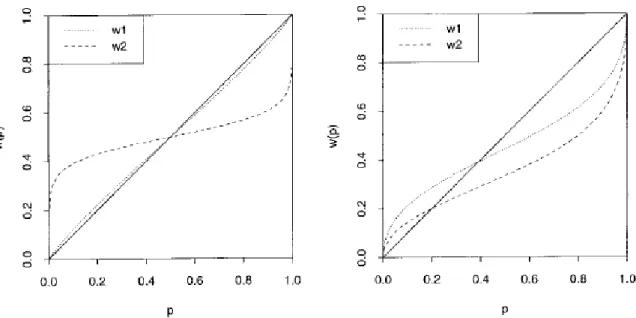
sensitiv-ity(curvature) and δ the elevation. When the weighting function is more elevated (higher δ) it implies less overall risk aversion for gains and more overall risk aversion for losses. The lower theγ the more pronounced the curve is, which implies more rapidly diminishing sensitivity to probabilities around the boundaries of 0 and 1, i.e., people become less sensitive to changes in probabilities as they move away from the reference point. See figure 2.2 to see the variations of
1
τdoes not have a psychological interpretation, so we use the delta which is a transformation ofτand where
the probability weighting function.
Note: On the left the weighting functions differ primarily in curvature. On the right weighting functions differ primarily in elevation
Figure 2.3: Variations of probability weighting functions
Another very known probability weighting function was proposed by Prelec (1998) which functional differs from the above since it uses the exponential.
w(p) =exp[−δ(−ln(p))γ] (2.10)
whereδ,γ >0. Whenδ= 1 the Prelec’s function collapses to a single parameter form: w(p) =
exp[−(−ln(p))γ].
up by Portuguese population, so this work which is inserted in a project that will be the first to identify the risk preferences for Portuguese individuals under the prospect theory. The ad-vantage of having a deeper knowledge about an individual’s preferences is that it enables the financial institution to better understand what level of risk a person is willing to take.
The loss aversion coefficient has an additional role in this study. Besides giving more in-formation about risk preferences of an individual, it also fulfils a secondary objective which is to find a relation with the DOSPERT scale2. The biggest advantage of finding this relation is
in the amount of work that each method requires. To calculate the coefficients of the prospect theory function, a large amount of work is required whereas the DOSPERT scale is easier to apply and making the task of determining which kind and amount of risk a person is willing to take much easier to the financial institution
2
3.
Data & Methodology
The primary objective of this work is to estimate the functional forms of the CPT as regards to the Portuguese population and the demographic differences that influence these same func-tional forms. For that we need to develop a specific survey that will provide us the information we need for the objective we have in hands. However it is very difficult to obtain a big enough sample that can replicate the heterogeneity of the Portuguese population, so we decided to ob-tain a sample using the Portuguese students from the Instituto Superior de Economia e Gest˜ao (ISEG). Only after collecting all the information we need, can we actually start to analyse and test which kind of curves and demographic properties the group has.
This chapter is divided in two sections, the first concerns the survey, how the questions were formulated and some aspects we needed to take into consideration so the responses would not deviate from the objective of the questions. The second part of the chapter is where we explain how results were treated and how we obtained the coefficients we proposed to study and the respective curves.
3.1
Survey
The experiment was conducted by an online survey to all students from ISEG. In most cases this kind of survey is made in a laboratory experiment because usually the frequency of errors in the lab experiment is drastically low, and so the results are more reliable. However Von Gaudecker et al. (2008) showed that the differences between the results obtained in a lab experiment or through an Internet platform are due to the selection of the candidates and not to implementation mode. So as long as the Internet experiment has the same participant selection as when the experiment is made in a lab, this problem can be overcome.
two options to select, “save”and “play”. The intention was to get the respondent to indicate his preferences, and choose for each outcome displayed whether he would prefer to save that amount and not play the game or if he would prefer to discard the amount and take a chance on the game. Once the preferences were selected, four new sure outcomes were presented linearly spaced between the lowest value on the saving side and the higher choice on the playing side. After selecting the new preferences with the same rule described above, the mid point of the lowest value on the saving side, and the higher choice on the playing side was displayed on the screen. This mid point is considered the certainty equivalent (CE).
We used the same procedure for the prospects in the loss domain, that is, when the game was presented to the respondent he had to choose for each outcome if he would prefer to pay that amount in order to avoid the possibility of having to pay a higher amount or if he would like to gamble having the possibility of paying the higher amount or nothing. Finally, to link the preferences of the gain domain with the loss domain it was necessary to estimate a certainty equivalent with a mix prospect. To do so, the game had to include a gain and a loss outcome. So in the survey two games were presented to the respondent; fifty-fifty chance of losing 20AC or
gaining 50AC, or fifty-fifty chance of losing 50AC or gaining an amount chosen by the respondent.
This amount chosen by the respondent have to turn this two games indifferent between them. Appendix A.1 is a Portuguese explanation of the survey sent to the students.
This first part of the survey had seven games for the gain domain from where we could calculate the functional forms of gains, seven games for the loss domain from where we could calculate the losses functional forms and just one game for the mix prospect. The reason why it was only necessary to ask one question for the mixed prospects is due to the fact that from all the other fourteen questions we could obtain all the coefficients that we need except for the loss aversion coefficient. So using the same approach as Abdellaoui et al. (2008) we only need one equation to extract the loss aversion coefficient and thus one mix prospect game. However a more detailed explanation is in the next section where we show the methodology we used to calculate the loss aversion coefficient.
We decided not to use monetary incentives in accordance with Camerer and Hogarth (1999) arguments and not due to budget constrains. They had said that “The data shows that incentives sometimes improve performance, but often don’t”. They also said that incentives have a great impact in surveys that require a mental effort like memorising and problem solving. However in surveys that require only intuition, incentives can hurt the results because thinking harder can distort our preferences. As choosing between risky choices is not a matter of cognitive function but is about intuition so incentives will not affect mean performance. For these reason incentives were not introduced into this survey, but the implication was a smaller number of questions so respondents would not be discouraged and continue responding until the survey was completed. There was a particularity on the survey. It could not prevent dominance violations. So after collecting all the results it was necessary to delete the inconsistent observations. An inconsistent observation is when the value of the sequence of stated outcome, for each individual, is not strictly increasing. For the mixed prospects the rejection rule was for all observation where the value input by the respondent was lower than the expected value. The down side of this approach is when a person makes one single mistake the entire observation is lost which implies rejecting a great number of observations. The up side of this approach is if an individual is consistent, that is, respects the dominance, it is plausible to admit that the respondent completely understood the questions, and his results will be highly reliable. So although there could be a large number of rejected observations and thereby obtaining a small sample, we can assume that the remaining observation are of excellent quality.
There was a second and a third part of the survey. The second part regards the DOSPERT-scale and it will be explained in a chapter further ahead. The third part of the survey relates to questions of the personal domain (e.g. age, gender and others).
3.2
Methodology
The CPT functional forms were calculated using the data obtained from the survey. As so, it was necessary to make a thorough description of the methodology used to calculate the coefficients for the probability weighting function, the value function and also the model used to study the relation with the demographic variables.
same. The first thing to do is to retrieve the certainty equivalents (c) that were obtained in the first part of the survey. Each question has a game like (x, p; 0) so using the 2.3 equation and disregarding the value function, it is possible to reduce the same equation to simpler one, as below:
w(p) =c/x (3.1) Using the first part of the survey and applying the 3.1 equation it is possible to obtain seven points of the probability weighting function. Once these seven points are calculated it is possible to make a regression in order to estimate the parametric values of the probability weighting function. The parametric form used was the proposed by Lattimore et al. (1992) (equation 2.9)
After calculating the coefficients of the probability weighting function we can proceed to the calculation of the value function. The elicitation of this function was divided into three stages. The first step was to calculate the utility function in the gain domain hence using only the positive prospects. Once again it is necessary first to calculate the points that are in the value function in order to be able to apply the functional form. The points used in this approach were the same as used in the estimation of the probability weighting function with the difference that
w(p) are the values obtained by the weighting function estimated previously. Using the equation 2.3 and 2.7 (in the gain domain) and taking into account that u(0) = 0 and to use the power function it is necessary to scaleu(1) = 1, the regression used was:
w(p) = (c/x)α (3.2)
The second stage is to calculate the utility curve in the loss domain. To do so, we use the same method as used in the gain domain, with the difference that now the scaling isu(−1) =−1 and is theβ coefficient that is being calculated. To calculate this parameter the prospects used were the negative ones, i.e. prospects like (y, p; 0) wheny <0.
The third and the last step is to measure the loss aversion coefficient. For this coefficient the mixed prospect was used. This prospect is like (x, p;y) when x > 0 and y < 0. In the third part of the survey it was asked an amount (k) that made two mixed prospect equivalent ((x1, p;y1)⇔(k, p;y2)). Using the value function for mixed prospects it is possible to write the
functional form of K¨obberling and Wakker (2005) with the power form it is possible to simplify to:
U(y1)w(p)−+U(x1)w(p)+=U(y2)w(p)−+U(k)w(p)+
−λ(−y1)βw(p)−+xα1w(p)+=−λ(−y2)βw(p)−+kαw(p)+
−λ(−y1)βw(p)−+λ(−y2)βw(p)−=−xα1w(p)++kαw(p)+
λ((−y1)βw(p)−+ (−y2)βw(p)−) =−xα1w(p)++kαw(p)+
λ=w(p)
+(kα−xα
1)
w(p)−(yβ
2 −y
β
1)
(3.3)
Once w(p)+, w(p)−, α and β are already calculated, λcan be easily calculated. This value
to the loss aversion coefficient is what Tversky and Kahneman (1992) had implicitly proposed, and is defined as −UU((1)−1).
So far we have assumed that there are two probabilities weighting functions, and two value functions, however al Nowaihi et al. (2008) affirmed “preference-homogeneity and loss-aversion are necessary and sufficient for the value function to have the power form with identical pow-ers for gains and losses and for the probability weighting functions for gains and losses to be identical”. Preference homogeneity1 essentially implies that when all prizes in a lottery are
scaled up by a factor, say k, then the certainty equivalent of the lottery is also scaled up by the same factor k (c(kf)=kc(f)). Tversky and Kahneman (1992) already affirmed that if the power value function of the form presented on equation 2.6 holds, then preference homogeneity is necessary and loss aversion implies thatλ >1. Hence from this paper it is possible to retract that α=β andw(p)+ =w(p)−. As so, if we based our study in this latter theory, we do not
need to calculate the functions for the loss domain, which will drastically decrease the amount of calculation required.
Finally to conclude the methodology for our first objective, we used a linear regression to estimate which demographics variables have an impact in the prospect theory parameters. The procedure used started by input all the demographic variables and secondly withdraw the variable which presents a higher p-value. This procedure continues until all the variables have a p-value lower than 10%. The only coefficient that does not oblige to this rule is the constant. In the next section, we will provide the results for our first objective, this is, the coefficients of CPT with a Portuguese sample. And also the results for the demographic variables.
1
4.
Results
After performing the survey the first thing we need to do is remove the inconsistent obser-vations. This is, remove the observations that did not present a strictly increasing sequence of outcomes regarding the prospects with gains and losses. In the loss aversion coefficient we reject the choices that are below the expected value of the game. Removing from the sample the inconsistent observations, from our sample of 159 responses only 31 (≈19%) held to be totally consistent for the prospects in the gain and loss domain and also the mix prospect. On the other hand, with the al Nowaihi et al. (2008) approach, there is no need to reject the inconsistencies from the losses. Hence, we get a total of 33 consistent observations (≈21%).
In table 4.1 we show the statistics of the demographic variables. From this table we can highlight that the sample is mostly constituted by males, aged between 18 and 23 years old, that have finished the bachelor degree. Is no surprising that most of the students are from economics, once the survey was implemented in an economics school.
Table 4.1: Sample statistics
Variable Observations Percentage (%) Gender
Male 19 61.3
Female 12 38.7
Age
18 to 23 19 61.3
24 to 30 8 25.8
>30 4 12.9
Education
Undergraduate 6 19.4 Bachelor’s degree 15 48.4 Masters degree 6 19.4 Posgraduated degree 4 12.9 Area of education
Economics 27 87.1
Sciences 4 12.9
Note: The table represents the sample distribution in terms of demographic variables. Each variable sums the 31 observation (100%).
answer for each game. It is interesting to notice that almost all games in the loss domain are higher (in absolute value) than the respective game in the gain domain. From here we can already conclude that, for this sample, people are more risk taking in the loss domain that in the gain.
Table 4.2: Certainty equivalent median Probability
Outcome (AC) .05 .10 .25 .50 .75 .90 .95
(50,0) 8 25 40
(-50,0) - 10 - 25 - 39
(100,0) 8 24 58 78
(-100,0) - 12 - 30 - 66 - 88
Note: The two outcomes of each prospect are given in the left-hand side of each row; the probability of the first outcome is given by the corresponding column. For example, the value of 8AC in the upper left corner is the median cash equivalent of the prospect (50AC, 0.10; 0, 0.90).
The median for the mixed prospect is 125 which is possible to denote that the gains must be at least twice as large than the losses. This implies that the loss aversion coefficient should be around 2. This is compatible with a value function that changes the slope abruptly at zero.
4.1
Functional forms
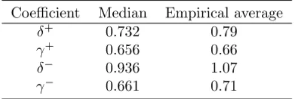
For the probability weighting function the δ and γ were estimated and the median of the results are displayed in table 4.3.
Table 4.3: Estimated coefficients: Probability weighting function Coefficient Median Empirical average
δ+ 0.732 0.79
γ+ 0.656 0.66
δ− 0.936 1.07
γ− 0.661 0.71
The median of the coefficients estimated for each valid observation. The empirical average is obtained by the average of the median for each coefficient which other authors have find.
with a p-value=.226.
It was also tested if the median of δ+ could be equal toδ− andγ+ toγ− and the results of
the sign test were the same for the two test, and both did not have significantly different medians (z=-1.510, p-value=.131 and z=-1.348, p-value=.177 respectively). When testingδ+ > δ− the
test was rejected at 10% (p-value=.066), meaning that the probability weighting function for the losses is more elevated then the gains which are shown on figure 4.1. Which in psychological terms means that people are more willing to take risk in the loss domain than in the gain domain. The hypotheses ofδ+ being higher than one was rejected with a 10% confidence (z=-1.300, p-value=0.097). This implies subcertainty which is a property presented by Kahneman and Tversky (1979). Subcertainty is when decision weights of complementary events sum less then one (w(p) +w(1−p)<1). Noting that the median ofw+(0.5) = 0.424 we can prove that
there is subcertainty. This value is very close to Tversky and Kahneman (1992) which is 0.421, and they are not significantly differences (z = 0.201, p-value = 0.955).
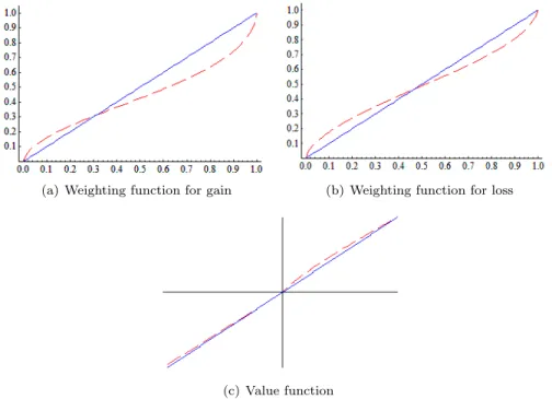
When both parameter ofγwhere tested to be higher or equal to one the null hypotheses were rejected (z=-10.090; p-value=.000 for gain and z=-6.632; p-value=.000), so it can be assumed that these parameter are lower than one. Since the inverse S-shape of the probability weighting function can only be achieved if γ <1 it is possible to assume that both weighting functions that were calculated in this work have an inverse S-shape. It is also possible to see this in figure 4.1.
After studying the coefficient of the probability weighting function, we studied the value function coefficients. The estimated values are displayed on table 4.4.
It was tested if the coefficients of the power function could be equal to one and the result was thatαwas rejected (z=-3.652; p-value=.001) butβ was not (z=-.681; p-value=.503). This mean that the value function can be linear in the loss domain, but we are sure that it is not linear for the gain domain. Thus, we need to test ifαcould be lower than one, in order to conclude about the concavity in the gain domain. This hypothesis was not rejected (p-value=1.000). Having said this it is possible to conclude that the value function in the domain of gain is concave but in the loss domain is near to the linearity.
Table 4.4: Estimated coefficients: Value function Coefficient Median Literature Average
α 0.886 0.78
β 0.972 0.87
λ 1.256 2.01
. The median of the coefficients estimated for each valid observation.
et al. (2005) and Abdellaoui et al. (2008)) hence our estimates fall within the range of recent estimates that find the power of the value function to be between 0.8 and 1.0. To test if the previous statement is true the same test of equality of means were made but now with the average value of the three last papers presented on the appendix A.2. So the test with the recent mean did not rejected the equality of the means (z=-,209 p-value=.837 and z=0,087 p-value=.931 respectively) confirming the statement and making our results in line with the literature.
The last test made to these two coefficients were if their median were equal (α=β). Once the test was not rejected (p-value=0.189) the hypothesis only one curve existing for gains and losses, proposed by al Nowaihi et al. (2008), may be sustained.
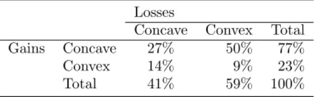
A classification to the utility functions was also made, to verify the proportion of the possible utility shapes. The rule to calculate this was, all the observation with anαlower (higher) than one are concave (convex) in the domain of gain. In the domain of loss, all the observation with aβlower (higher) than one are convex (concave). We did not include the possibility of linearity because neither coefficients could be exactly one. The table 4.5 demonstrate the respective proportion.
Table 4.5: Classification of respondents Losses
Concave Convex Total Gains Concave 27% 50% 77% Convex 14% 9% 23% Total 41% 59% 100%
Note: A value function that is concave for gains and convex for losses have aα <1 andβ >1 respectively. The reasoning is the same for other possible value functions.
the gain domain 77% of the observation are concave, which increases the credibility that the utility function has to be concave in the gain domain. However it is not possible to take the same conclusion for the loss domain once the probabilities are quite balanced. With this kind of results it is possible to conclude that the value function in the loss domain is closer to the linearity.
There is still one coefficient remaining to conclude the first part of our work, the loss aversion coefficient. Theλestimation was 1.256. This value is lower than the empirical average and when tested if they were equal, the hypothesis was rejected at 5% level (z=-2.146; p-value=.040).
Despite the literature average is around two, recent findings, show that the value of λ is lower than two showing once again that this result is in agreement with the contemporaneous works (Abdellaoui et al. (2008) and Booij et al. (2010)).
(a) Weighting function for gain (b) Weighting function for loss
(c) Value function
Note:The red dash line is the prospect theory functions and the blue solid is 45o
line
Figure 4.1: Estimated functions of prospect theory
results a bit more robust. The table below shows a big difference between this new approach, of using the same coefficients in the loss domains as in the gain domain. This one presents aλ
around 2. Which is much closer to the empirical mean.
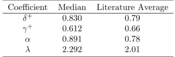
Table 4.6: Estimated coefficients: Second approach Coefficient Median Literature Average
δ+ 0.830 0.79
γ+ 0.612 0.66
α 0.891 0.78
λ 2.292 2.01
The median of the coefficients estimated for each valid observation. The empirical average is obtained by the average of the median for each coefficient which other authors have find.
Bothδ+andγ+were significantly equal to their literature mean (z=1.036, p-value= .300 and
z=0.342, p-value=,732 respectively) andαwere not significantly equal to the literature average (z=5.688, p-value=.000), but it was significantly equal to the contemporaneous mean (z=-.537, p-value=.591). λ is not significantly equal to the average values of the empirical estimations. However when testing ifλ <2 the test was rejected (z=3.134, p-value=.000) meaning that there is some evidence that losses look twice larger than gains. This value is more in line with the literature, however, as we said before, recent studies prooved that this value is in fact lower than two.
4.2
Demographic Model
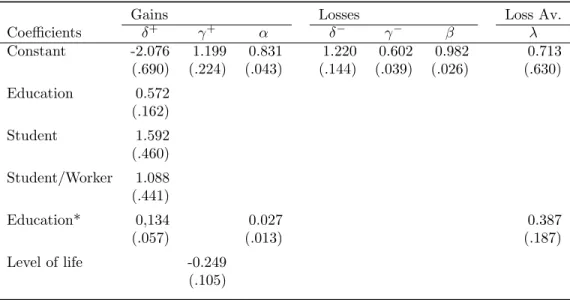
The results of the linear regression for the demographic variables are presented on the table 4.7. This table only shows the significant variables for each coefficient. All the non significant variables were removed from the analysis.
It is possible to notice, that education, occupation and parents education of each individual have a positive impact on the elevation of the probability weighting function in the gain domain. The interpretation of these variables are that people with higher education, less experience of work and parents also with high education are more willing to take more risks in the gain domain.
Table 4.7: Linear Regression for the Demographic Variables
Gains Losses Loss Av.
Coefficients δ+ γ+ α δ− γ− β λ
Constant -2.076 1.199 0.831 1.220 0.602 0.982 0.713 (.690) (.224) (.043) (.144) (.039) (.026) (.630) Education 0.572
(.162) Student 1.592 (.460) Student/Worker 1.088 (.441)
Education* 0,134 0.027 0.387
(.057) (.013) (.187)
Level of life -0.249 (.105)
* Variables are related to the parents
Notes: Standard errors in parenthesis. All this values are significantly at least 10%
it is possible to conclude that these results are in line with the literature. Assuming that the parents education have the same interpretation as the education of an individual, it will be also expected that the variable would have an impact on the elevation of the probability weighting function. As shown in the previous table, this variable has indeed an impact on the elevation in the gain domain but not as big as the education of the individual, for more detail about this subject see Dohmen et al. (2005). There is also some evidence, in the gain domain, that a full-time student is more willing to take risks than a student who also works and even more than a working person. It is possible to conclude that a person which works for their money has a bigger feeling of ownership than a person which gets his money from his parents. A student is therefore more willing to take risks (biggerδ−) than a worker. With this new evidence it is
possible to actually see in practice theendowment effect.
The sensibility of the probability weighting function in the gain domain is given by the level of life. This value can be seen in the γ+ coefficient. As seen before, the higher the value of
this coefficient the more close to the linearity the function is, which means the less sensitive the person is in changes of probability. Taking table 4.7 in consideration it is possible to notice that a person with better conditions of life is more sensitive in probabilities changes.
shape form. An explanation for this could be that a person with more money is not so sensitive as a non wealthy person. A small change on the probability does not have much of an impact once the outcome that could result from that prospect does not make a big change on the quality of life from that person. On the other and, a non wealthy person, have the same impact for all level of probability, once any increase on the probability of winning, as little as it could be, will have a positive impact on the quality of life for that person. Although this interpretation could be correct, there are no other study which supports this. So to make this coefficient more robust more studies about this should be made. Also this coefficient is not very reliable since it resulted from questions aimed at understanding the level of life respondents perceive to have, and was not made in terms of a numerical conclusion, like the IRS scale1. Unfortunately there
is no evidence of which kind of characteristics have an influence on the probability weighting function in the loss domain. Booij et al. (2010) also stumbled with this problem. So, there is evidence that in the loss domain there is no heterogeneity among the respondents.
The curvature of the value function in the domain of gains is measured by the αand this coefficient is dependent of the parents education. Once this value is positive it means that the higher the parents education, the higher theα, which implies a less concave function. Once the concavity is related to risk aversion it means that people are more willing to take risks if their parents had the opportunity of high levels of education which can be related to the life style they could provide to their children. Once again there is no evidence that there is a relation between the demographic variables and the curvature of the value function in the loss domain. Finally, it seems that the loss aversion coefficient has a positive relation with the parents education. As described before, a person with an higher loss aversion means that it has to gain more for each unit that he might loose. This result is not in line with the findings of Booij et al. (2010), they find that education is associated with a lower degree of loss aversion.
Taking into account al Nowaihi et al. (2008), we will also apply the demographic model when the loss coefficients are equal to the gains. The major implication of the results, is because we have a bigger sample which makes our results a bit more robust.
Comparing table 4.7 with 4.8 it is possible to notice that both econometric models point to the same results. However there are two differences. In this last studyαhas no evidence that is explained by the parents education, and also, that the loss aversion coefficient is not explained
1
also by parents education but its explained by gender (male). Booij and van de Kuilen (2009) affirms that the females are more loss averse than males but table 4.8 presents a different result, whereby males have a larger loss aversion coefficient than females. So this last result is not in line with the literature, so further investigation should be made in order to understand what cause it.
Table 4.8: Linear Regression for the Demographic Variables: Second approach Gains Loss Av.
Coefficients δ+ γ+ α λ
Constant -1.274 2.172 .899 2.025 (.636) (.707) (.021) (.130)
Male .333
(.159) Education .478
(.149) Student 1.035 (.455) Student/Worker 1.035 (.437)
Level of life -0,151 (.070)
5.
CPT Applications
Up to now, we have shown how the cumulative prospect theory describes the risk preferences of a Portuguese sample and some demographic differences between those preferences, which by itself is an important step to improve our knowledge about the risk decision made by the Por-tuguese. However, if we want this theory to have a bigger role in measuring the risk preferences of an individual it is extremely important to simplify the calculations presented in section 3.2. As so, in a partnership with Silva (2012) we try to find a relation between the loss aversion coefficient and the DOSPERT-Scale. This linkage between CPT and the DOSPERT-scale is not enough to apply this theory to the financial markets. The theory that is commonly used to choose the efficient portfolio, better known as ”Portfolio Selection” by Markowitz (1952) is based on the expected utility theory so it is necessary to adapt it to the cumulative prospect theory.
By overcoming these two obstacles it is possible for financial institutions to apply this theory with a small price of implementation through the DOSPERT-scale and correctly find the market efficient portfolio when the portfolio selection is adapted to the CPT. The next sections will demonstrate how this can be accomplished.
5.1
CPT and DOSPERT-Scale
obtain the risk coefficient the survey described in section 3.1 had a second part consisting of thirty questions where each individual had to respond for each situation, the possibility of they perform a specific behaviour, in a scale from “1-Extremely Unlikely”to “7-Extremely Likely”. Making the average, per domain, of the thirty questions, we can obtain a result from 1 to 7, with 1 being the more risk averse possible and 7 being the more risk seeking possible.
Silva (2012) have found evidence of relation between the loss aversion coefficient with the financial (0.334) and gamble (0.320) sub-domain coefficient both statically significant at 10% but for the risk coefficient and the investment sub-domain coefficient the relation was low and it was not statistically significant. With this first result we believe that it is possible to find a relation with the financial and gambling coefficient and not to the risk and investment. As it was expected there is a linear relationship between the financial coefficient which is significant at 10% (p-value 0.047),withR2 of 0.111 and F-Statistic of 4.263 and there is also evidence of
a linear relationship with the gamble coefficient statistically significant at 10% (p-value 0.057), withR2 of 0.102 and F-Statistic of 3.870.
λ= 0.775 + 0.334F inancial+ǫ (5.1)
λ= 0.877 + 0.320Gamble+ǫ (5.2) This confirms that there is indeed a relationship between the financial and the gamble co-efficient from the DS with the loss aversion coco-efficient from the CPT. On the other hand there was no evidence of a relation with the risk and investment coefficients which makes possible to make an interesting conclusion. If we can find a relation with the gamble coefficient and not with the investment decision it is possible that the questions from where we obtained the loss aversion coefficient triggers gambling decisions and not investment ones which was what we intended. March and Shapira (1987) explained that managers differentiate between investment and gambling decisions once the first involves decisions which requires a deeper reflection on the decision making process and the later is based on luck. This conclusion obligates a deeper study about the difference between this two domains and will probably require a reformulation of the questions that usually are used to estimate the prospect theory coefficients.
5.2
CPT and Mean Variance Applications
Once we overcome the difficulty of the loss aversion calculation we can turn our attention to the next problem, the fact that theories involving the selection of the efficient portfolio are based on the EUT. As stated, this theory does not fully explain the decisions preferences of individuals. So, as the last objective of this work we will demonstrate the impact on the investments decisions of an individual if we start using the CPT over the EUT. For this we will adapt to the CPT, the most known investment decision rule under uncertainty, the Markowitz (1952) Portfolio Selection.
The portfolio selection theory relies on an assumption that investors are interested in max-imising the return for a given risk or, minmax-imising the risk for a given return, which essentially is the mean-variance rule (MV). Levy and Levy (2004) defined the MV rule as:
Definition 1 An investment F dominates G by MV if the expected value of investment F (µF)
is larger than G (µG) and the standard deviation of F (σF) is equal or lower than G (σG). Note
that under normal distributions and risk aversion MV rule coincides with EU maximisation (Markowitz (1952)).
µF ≥µG and σF ≤σG (5.3)
As the Portfolio Selection theory assumes normal distributions and the MV-rule, it is fair to assume that the EUT is on the foundation of this theory, which Kahneman and Tversky (1979) have proofed that individuals systematically violate. So we need a new decision rule that correctly describes the individual preferences demonstrated by Tversky and Kahneman (1992), known to have a S-shape value function and an inverse S-shape probability weighting function. Levy and Levy (2004) have proposed a definition for this kind of curves called the Prospect Stochastic Dominance (PSD).
Definition 2 Investment F dominates G for all S-shaped, non decreasing utility function (U′(X)>
0 for all x6= 0, U′′(X)>0 for allx <0, and U′′(X)<0 for allx >0) if the area enclosed
between the two cumulative distributions is positive for any range [x,x¯] withx≥0 andx¯≤0.
Z ¯x x
In a more intuitive way, an investment F dominates G by the MV-rule if F have a higher expected return and lower standard deviation as G. On the other hand F dominates G by the PSD-rule if the cumulative distribution function (CDF) of F is to the right of G, this is,
Rx¯
x [G(z)−F(z)]dz > 0. So, on the first sight, the MV and PSD dominance have no direct
relationship, i.e., one investment can have dominance by MV but not by PSD, or vice versa. In appendix A.4 there is a figure which demonstrate both situations. However, in portfolio context, Levy and Levy (2004) as proved that both stochastic rules have a very close relationship. They had presented the following theorem1when we assume the investors do not have distorts probabilities.
Theorem 1 The PSD-efficient set is a subset of the MV-efficient set, and the segment of the MV-efficient set which is excluded from the PSD-efficient set is at most the segment between the minimum variance portfolio and the point of tangency from the origin to the frontier.
Figure 5.1: The MV and PSD efficient frontiers
This can be intuitively proved because, for one inefficient investment (F’) there is always another with the same standard deviation but with a higher expected return (F), so it is obvious that F dominates F’ by the MV rule and it also dominates by the PSD rule once the CDF of F is the same as F’ but deviated to the right. And since the efficient frontier between the minimum variance portfolio (O) and the point of tangency from the origin have steep slope (a),
1
a small increase in the standard deviation is a big increase in the expected return, so the CDF of the tangency portfolio will always be to the right of the portfolios below. Passing the point of tangency the slope of the efficient frontier decrease, so the portfolio are no longer dominated by portfolios to their immediate right (see figure 5.2).
However, we ca not disregard the distortions of probabilities. As proved by Tversky and Kahneman (1992) and also by the empirical study made in this work, the probability of an outcome does not have a direct relation with the perception of a probability by an individual, it as indeed a distortion. So Levy and Levy (2004) proposed a second theorem2.
Theorem 2 The objective probabilities are subjectively distorted by any transformation that does not violate first-degree stochastic dominance, for example, the cumulative prospect theory transformation. Then, the PSD-efficient set is a subset of the MV-efficient set.
Since the probability transformation may change the perceived portfolio mean and standard deviation, it is not possible to restrict the MV to the PSD efficient curve as it was possible with the objective probabilities. So a portfolio that is PSD efficient with objective probabilities can be PSD inefficient when probabilities are transformed and vice versa.
5.2.1
The Empirical PSD efficient frontier
In this section we will apply this concepts to the Portuguese market to find the empirical PSD efficient frontier. We will use the stocks that are included in the Portuguese index (PSI-20) from September 2008 to September 2012, to produce the MV efficient frontier and then reduce it to the PSD efficient frontier.
To reduce to the PSD efficient frontier we start from the minimum variance portfolio and check if the portfolios to the right of them respect the PSD rule. To distort the probabilities we use the equation 2.9 using the results we have estimated in 4.1 which give us the following equation:
w(p) = 0.732p
0.656
0.732p0.656+ (1−p)0.656 (5.5)
Until the portfolio is dominated by another to the right it can not be included in PSD efficient frontier. The figure 5.2 presents the result we achieve with this methodology.
2
Figure 5.2: The PSD efficient frontiers
6.
Conclusion and Further Research
To the best of our knowledge, this study presents the first full estimation of the cumulative prospect theory for a Portuguese sample. There are a few studies that made this kind of work with a sample for different countries but it is interesting to know if the Portuguese follows this theory, and this study confirms that actually it follows. It has also the advantage of knowing the risk preferences from Portugal, allowing financial institutions to create financial products in line with these preferences.
From the results it is possible to see that for the sample of Portuguese students under analysis there is a S-shape utility function, concave in the gain domain and convex in the loss domain. However there is also some evidence that this last one is closer to the linearity than convexity which is in line with the most recent literature (Abdellaoui et al. (2008)). The coefficient of loss aversion is below the average comparing to the literature. However, taking into account the tests made, it is possible to say that the value of 1.256 is a good result in comparison with the recent literature. The probability weighting function shows indeed an inverse S-shape which was what it was expected and even more, the function for the loss domain is more elevated than in the gains, which implicates a pessimism in both domains. This is one more proof of the validation of cumulative prospect theory.
Our results seems to show some heterogeneity among the sample only in the gains domain. People with more education (personally or from their parents) and less experience of work (students and working students) are more risk seeking. On the other hand people with a lower level of life are more sensitive to changes in the probability.
A limitation of this work is the size of the survey. With a small number of questions, we do not make a very precise estimation of the CPT functional forms. With a few questions we had to rejected all the observation that had a single mistake. With a bigger survey we can allow the respondent to make one mistake thus having less number of rejected observations and therefore a bigger sample to work with. As so we suggest, for future research, a survey with more questions in every domain.
students of one single school which resulted in a sample with a low level of heterogeneity. It will be interesting to extend this study to a larger population, in order to take an inference from the Portuguese population, and also because it will turn the results more robust.
Another interesting subject for further research could be to define which is the method more correct to calculate the loss aversion coefficient. With the method where there is different function of gains and losses for the probability weighting function and the value function, or the method where the same parameters are assumed for both curves in loss and gain domain.
We also shown that it is possible to link the loss aversion coefficient with the DOSPERT-scale. This finding will improve the financial markets, and it will probably be the starting point of implementation of cumulative prospect theory in the portfolio choice domain. We have also extended this theory to the efficient frontier. As Levy and Levy (2004) proved, we find that the efficient frontier is smaller than what we are used to know. Taking into account the distortions of the probabilities, we have reduced the Portuguese market efficient frontier to one that is more suitable for our sample.
Bibliography
Abdellaoui, M. (2000). Parameter-free elicitation of utility and probability weighting functions.
Management Science 46(11), pp. 1497–1512.
Abdellaoui, M., H. Bleichrodt, and O. L’Haridon (2008). A tractable method to measure util-ity and loss aversion under prospect theory. Journal of Risk and Uncertainty 36, 245–266. 10.1007/s11166-008-9039-8.
Abdellaoui, M., H. Bleichrodt, and C. Paraschiv (2007, October). Loss aversion under prospect theory: A parameter-free measurement. Management Science 53(10), 1659–1674.
Abdellaoui, M., F. Vossmann, and M. Weber (2005). Choice-based elicitation and decomposition of decision weights for gains and losses under uncertainty. Management Science 51(9), pp. 1384–1399.
al Nowaihi, A., I. Bradley, and S. Dhami (2008). A note on the utility function under prospect theory. Economics Letters 99(2), 337 – 339.
Allais, M. (1953). Le comportement de l’homme rationnel devant le risque: Critique des postu-lats et axiomes de l’ecole americaine. Econometrica 21(4), pp. 503–546.
Andersen, S., G. Harrison, M. Lau, and E. Rutstrˆom (2006). Elicitation using multiple price list formats. Experimental Economics 9, 383–405. 10.1007/s10683-006-7055-6.
Bernoulli, D. (1954). Exposition of a new theory on the measurement of risk. Economet-rica 22(1), pp. 23–36.
Booij, A., B. van Praag, and G. van de Kuilen (2010). A parametric analysis of prospect theory’s functionals for the general population. Theory and Decision 68, 115–148. 10.1007/s11238-009-9144-4.
Camerer, C. F. and R. M. Hogarth (1999). The effects of financial incentives in experiments: A review and capital-labor-production framework. Journal of Risk and Uncertainty 19, 7–42. 10.1023/A:1007850605129.
Dohmen, T., A. Falk, D. Huffman, U. Sunde, J. Schupp, and G. G. Wagner (2005). Individual risk attitudes: New evidence from a large, representative, experimentally-validated survey. Framed Field Experiments 0019, The Field Experiments Website.
Donkers, B., B. Melenberg, and A. Van Soest (2001). Estimating risk attitudes us-ing lotteries: A large sample approach. Journal of Risk and Uncertainty 22, 165–195. 10.1023/A:1011109625844.
Fehr-Duda, H., M. de Gennaro, and R. Schubert (2006). Gender, financial risk, and probability weights. Theory and Decision 60, 283–313. 10.1007/s11238-005-4590-0.
Gonzalez, R. and G. Wu (1999). On the shape of the probability weighting function. Cognitive Psychology 38(1), 129 – 166.
Kahneman, D. and A. Tversky (1979). Prospect theory: An analysis of decision under risk.
Econometrica 47(2), pp. 263–292.
K¨obberling, V. and P. P. Wakker (2005). An index of loss aversion. Journal of Economic Theory 122(1), 119 – 131.
Lattimore, P. K., J. R. Baker, and A. D. Witte (1992, August). The influence of probability on risky choice: A parametric examination. Working Paper 81, National Bureau of Economic Research.
Levy, H. and M. Levy (2004). Prospect theory and mean-variance analysis.Review of Financial Studies 17(4), 1015–1041.
Levy, J. S. (1992). An introduction to prospect theory.Political Psychology 13(2), pp. 171–186. March, J. G. and Z. Shapira (1987). Managerial perspectives on risk and risk taking.
Manage-ment Science 33(11), pp. 1404–1418.
Silva, R. (2012). Risk profiling and the dospert scale: An approach using prospect theory. Instituto Superior de Economia e Gest˜ao.
Stott, H. (2006). Cumulative prospect theory’s functional menagerie. Journal of Risk and Uncertainty 32(2), 101–130.
Tversky, A. and C. R. Fox (1995). Weighing risk and uncertainty. Psychological Review 102(2), 269–283.
Tversky, A. and D. Kahneman (1992). Advances in prospect theory: Cumulative representation of uncertainty. Journal of Risk and Uncertainty 5, 297–323. 10.1007/BF00122574.
Von Gaudecker, H.-M., A. H. Van Soest, and E. Wengstr¨om (2008). Selection and mode effects in risk preference elicitation experiments. Working paper series, Institute for the Study of Labor (IZA).
Weber, E. U., A.-R. Blais, and N. E. Betz (2002). A domain-specific risk-attitude scale: mea-suring risk perceptions and risk behaviors. Journal of Behavioral Decision Making 15(4), 263–290.
A.
Appendix
A.2
Empirical estimates of prospect theory using different
parametric functionals
Functional form Estimates Properties* Authors
VF α β λ E T I N
v(x) =xα , ifx≥0 and−λ(−x)β, ifx <0
.88 .88 2.25 md c n 25 Tversky and Kahneman (1992) .50 ml c n 420 Wu and Gonzalez (1996) .49 md c n 10 Gonzalez and Wu (1999) .89 .92 md c y 40 Abdellaoui (2000) .61 .61 ml b n 2593 Donkers et al. (2001) .91 .96 md c n 41 Abdellaoui et al. (2005) .72 .73 2.54 md c n 48 Abdellaoui et al. (2007) .81 .80 1.07 ml c y 90 Andersen et al. (2006) 1.01 1.05 md c y 181 Fehr-Duda et al. (2006)
.86 1.06 2.61 md c y 48 Abdellaoui et al. (2008) .86 .83 1.58 ml m n 438 Booij et al. (2010) Average Values .78 .87 2.01
PWF δ+ γ+ δ− γ−
w(p) =pγ/(pγ+ (1−pγ))1
γ
.61 .69 c n 25 Tversky and Kahneman (1992) .71 c n 420 Wu and Gonzalez (1996) .60 .70 c y 40 Abdellaoui (2000) .76 .76 c y 90 Andersen et al. (2006)
w(p) =δpγ/δpγ+ (1−p)γ
.77 .69 c n 40 Tversky and Fox (1995) .77 .44 c y 10 Gonzalez and Wu (1999) .65 .60 .84 .65 c y 40 Abdellaoui (2000) .98 .83 1.35 .84 c n 41 Abdellaoui et al. (2005) .87 .51 1.07 .53 c y 141 Fehr-Duda et al. (2006) .77 .62 1.02 .59 m n 438 Booij et al. (2010)
w(p) =exp[−δ(−ln(p))γ]
.74 c n 40 Wu and Gonzalez (1996) .413 .413 b n 2593 Donkers et al. (2001) Average Values .80 .63 1.07 .65
A.3
Estimators value for each individual
δ+ γ+ α δ− γ− β λ
1 1,15 0,38 0,59 0,82 0,79 0,80 0,32 2 2,96 0,51 0,88 0,66 0,39 0,98 2,50 3 1,10 1,01 0,70 0,95 0,74 1,02 0,58 4 0,50 0,72 1,04 0,92 0,43 1,12 1,26 5 1,06 0,83 0,92 0,70 0,92 1,30 0,22 6 0,43 0,61 0,86 0,76 0,73 1,05 0,63 7 0,96 0,93 0,83 0,81 0,66 0,97 1,25 8 1,36 0,70 1,07 0,96 0,73 0,97 4,97 9 0,66 0,52 0,88 0,92 0,50 0,93 0,59 10 0,70 0,64 0,99 1,14 0,66 0,95 2,08 11 1,24 0,74 0,90 1,13 0,69 1,09 1,01 12 1,00 0,97 1,00 1,00 0,97 1,00 1,00 13 0,45 0,61 0,67 2,57 0,31 0,93 0,29 14 0,22 0,56 0,93 2,33 0,66 1,15 0,24 15 0,29 0,65 0,82 2,09 0,59 0,84 0,83 16 0,42 1,28 0,91 1,23 0,87 0,83 1,75 17 0,94 0,66 0,94 0,78 0,73 1,05 1,60 18 0,74 0,82 0,84 1,19 0,97 0,81 2,55 19 0,25 0,96 0,84 0,66 0,35 0,76 2,05 20 0,61 0,64 0,87 0,78 0,90 1,10 0,28 21 1,12 0,50 1,13 0,62 0,45 0,96 8,16 22 0,54 0,69 0,74 1,10 0,55 1,09 0,11 23 0,94 0,53 0,88 2,63 0,34 1,26 0,28 24 0,56 0,51 0,85 5,53 1,70 1,21 0,08 25 1,17 0,75 1,14 0,77 0,76 1,09 2,91 26 0,30 0,27 0,78 2,31 0,65 0,82 0,37 27 1,05 0,52 0,63 0,20 0,43 1,24 0,14 28 0,96 0,40 0,95 1,33 0,36 1,04 0,57 29 0,73 0,53 0,84 0,77 0,43 0,97 1,08 30 2,19 0,31 0,89 0,71 0,40 0,97 1,74 31 0,26 0,66 1,02 0,85 0,71 1,02 1,17
Median of