Article
Printed in Brazil - ©2014 Sociedade Brasileira de Química0103 - 5053 $6.00+0.00A
*e-mail: [email protected]
Validation Method to Determine Metals in Atmospheric Particulate Matter by
Inductively Coupled Plasma
Optical Emission Spectrometry
Luciana M. B. Ventura, Beatriz S. Amaral, Kristine B. Wanderley, José M. Godoy and Adriana Gioda*
Department of Chemistry, Pontifical Catholic University of Rio de Janeiro (PUC-Rio), Marquês de São Vicente, 225, 22451-900 Rio de Janeiro-RJ, Brazil
Material particulado atmosférico (PM) é um poluente composto por diversos metais, que quando acumulados no sistema respiratório, podem causar sérios problemas de saúde. Os métodos IO-3.1 (extração de metais em PM) e IO-3.4 [determinação de metais por espectrometria de emissão atômica por plasma acoplado indutivamente (ICP-OES)] são os recomendados pela Agência de Proteção Ambiental dos Estados Unidos. Com o objetivo de avaliar o desempenho do método desenvolvido em nosso laboratório para extração de metais em PM utilizando HNO3 p.a. bidestilado e determinação por ICP-OES de Al, Ca, Cd, Cu, Cr, Fe, K, Mg, Mn, Na, Ni, Pb, Ti, V e Zn, a validação foi executada de acordo com os critérios estabelecidos pelo INMETRO, determinando parâmetros: seletividade, linearidade, precisão, exatidão, robustez, limites de detecção e quantificação, assim como a comparação da eficiência e precisão com o método IO-3.1. Resultados mostraram que o nosso método atendeu todos critérios de validação estabelecidos pelo INMETRO. Além disso, mostrou-se ser equivalente ao método IO-3.1.
Atmospheric particulate matter (PM) is a pollutant composed by various metals, that when accumulated in the respiratory system may cause serious health problems. Methods IO-3.1 (metal extraction in PM) and IO-3.4 [metal determination by inductively coupled plasma optical emission spectrometry (ICP-OES)] are the recommended by the United State Environmental Protection Agency. With the intent to evaluate the performance of the method developed in our laboratory for the extraction of metal in PM with HNO3 p.a. bidistilled and determination by ICP-OES of Al, Ca, Cd, Cu, Cr, Fe, K, Mg, Mn, Na, Ni, Pb, Ti, V and Zn, validation was executed according to the criteria established by the INMETRO determining the parameters: selectivity, linearity, precision, accuracy, robustness, limits of detection and quantification, as well as the comparison of the efficiency and precision with IO-3.1 method. The results show that our method meets all validation criteria established by the INMETRO; furthermore, it shows to be equivalent to IO-3.1 method.
Keywords: validation method, PM2.5, ICP-OES, atmospheric chemistry
Introduction
Atmospheric particulate matter (PM) pollutant is regulated in Brazil by the National Environment Consul
through Resolution No 03/1990.1 This resolution
establishes the limit of daily exposure (average of 24 h) and continued exposure (annual average) to particulate matter in suspension (PTS) and inhalable particulate matter (PM10). However, no limits were established for
fine fraction (PM2.5), therefore, studies are indispensable to create an inventory.
Since the eighties, researchers2-5 had already noticed
Besides the relation of metals present in particulate matter with health issues, it is possible to determine their connection with their source of origin, for example: natural, with the re-suspension of soil and marine aerosols and anthropogenic. Moreover, when receptor models are used, it is possible to identify if they are originated from fossil fuels operated by thermoelectric plants, steel mills,2 or
vehicles6 which contribute to the degradation of air quality
in a certain region.7,8
The determination of metal concentration in atmospheric particulate matter allows governments (federal, state and local) to execute control actions to reduce the impacts caused on human health. The advent of inductively coupled plasma (ICP) spectroscopy improved the performance and velocity of metal analysis in various ICP applications, being able to quantify metals on levels that are required by environmental laws.9
Brazil still has not defined the limit for metal concentration present in the air. Nevertheless, some countries already monitor and regulate metals present in particulate matter. Nonetheless, numerous methodologies are found in literature for the characterization of metals in PM.6-10 The most used methodologies are the recommended
by the United State Environmental Protect Agency (U.S. EPA): method IO-3.111 (extraction of metals in PM)
and IO-3.49 [metal determination by inductively coupled
plasma optical emission spectrometry (ICP-OES)]. However, utilization of different analytical methodologies requires validation to ensure the efficiency of the method.
More and more laboratories seek to obtain analytical results that can be compared traceable and trusted otherwise they may lead to disastrous decisions and irreparable financial damage.12 Validation aims to demonstrate that
an analytical method, in the conditions which it regularly takes place, possess the necessary characteristics for the obtainment of reliable and consistent results and contains the quality required for the application for which it is intended.13,14 According to National Health Surveillance
Agency (ANVISA),15 validation should ensure, through
experimental studies, that the methodology meets the requirements of analytical applications, ensuring the reliability of the results.
Standardized methods, in general, have the following parameters pre-determined: selectivity, linearity, working range, precision, accuracy, recovery, robustness, limits of detection and quantification; validation execution is not required. However, analytical methods developed by the laboratory, methods not normalized, standard methods used outside of the scope for which it was designed or even extended or modified methods in relation to the standard do not have the parameters mentioned above. Therefore
validation is required to ensure that the performance characteristics of the method meet the requirements for analytical operations intended, generating reliable and interpretable information about the sample.12,13
As well as the guides/resolutions available by national agencies for the validation of analytical methods, there are some defined/elaborated by international organizations such as International Conference on Harmonization (ICH)16
for pharmaceutical appliances, the International Union of Pure and Applied Chemistry (IUPAC)17 which registered
a technical document that has been used by ISO18 through
the international norm ISO/IEC 17025 which is a specific norm for testing and calibration laboratories, and the United States Food and Drug Administration (US-FDA)19
for foods and pharmacies in the United States. However, such agencies13,15,16,18,19 and others require the validation
of analytical methods item as a fundamental requirement for quality certification and demonstration of technical competence of the laboratory.12
The validation of a method is a continuous process that begins in the planning of the analytical strategy and continues throughout all its development. Thus, it is a long process and requires a large number of tests and statistical calculations resulting in a high cost analysis. Therefore, it is necessary to select the parameters that have a greater impact on the quality of the results and the speed in which they are obtained. For that reason, it is not always economically relevant to conduct all the validation testes suggested in the guides found in literature.20-23 The objective of this study
was to validate a methodology developed in our lab in order to determine metals in particulate matter by ICP-OES.
Experimental
It is possible to find in literature various methodologies for the determination of metals in particulate matter.6,7,9,10
To evaluate the performance of the analytic procedure developed in our laboratory by Gioda et al.24 to determine
metals by ICP-OES, we selected some metals from different sources: Al, Fe, Ti, Mn, Mg (soil), Na, Ca (marine aerosol), Cd, Cu, Cr, Zn (industrial), K (biomass burning), Ni, Pb and V (vehicular). The metals were extracted from the PM with HNO3 p.a. bidistilled and the validation was executed
according to the criteria established by INMETRO.13
Materials
Sarstedt, micro and automatic macropipettes from Kacil (± 1%), dispenser Distrivar (± 5%), beaker and volumetric flask were used in the sampling, extraction and analysis procedures.
Reagents
The reagents used were: multielement standard solution Certipur Multielement Standard IV, 1000 mg L−1 by Merck
(Ag, Al, B, Ba, Bi, Ca, Cd, Co, Cr, Fe, Ga, K, Li, Mn, Ni, Sr, Na, Cu, In, Mg, Pb, Tl, Zn), and standard monoelementares of V and Ti 1000 mg L−1 Titrisol® by Merck, bidistilled
nitric acid p.a. (16.8 mol L−1 HNO
3) by Merck, hydrochloric
acid p.a. (12.0 mol L−1 HCl) by Merck.
Equipments
An ICP-OES Perkin Elmer, USA, model: Optima DV 7300, High Volume Sampler (AGV), Energética S.A, BRA, model: AGVMP252, analytical balance Scientech Model: SA 2.0 (± 0.0001 g), heating block Fisaton and centrifuge Fanem LTDA (150 µA) were used.
Sampling
Fine particle matter (PM2.5) samples were
collected in downtown of the city of Rio de Janeiro (22º54’26.67’’/43º11’43.13’’) during 2011. The samplings were performed in 24 h periods, every six days, using high volume sampler and glass fiber filters, according to NBR 13412 method. An average flow of 1.16 m3 min−1
was used. The PM2.5 concentrations ranged from 12 to 40 µg m−3, with an average of 25 ± 11 µg m−3. The PM
2.5
mass collected in the filters ranged from 0.02 to 0.06 g.
Experimental procedure
The analytical procedure can be divided into two stages: acid extraction with bidistilled concentrated nitric acid and determination by ICP-OES of metals in atmospheric particulate matter. The careful execution of each step determines the quality of the results obtained in the process as a whole.
Metal extraction from atmospheric particulate matter
To accomplish the extraction of metals, 7 blank filters and 7 PM2.5 samples were used. An aliquot (9 cm2, m ca.
0.08 g) of each filter was cut with Teflon scissors, placed
inside polypropene tubes and added 3.0 mL of HNO3
(16.8 mol L−1) bidistilled. These tubes were closed and
heated for 2 h at 95 ± 5 °C. After that, the tubes were left to cool down to room temperature and were diluted to 25.0 mL with MilliQ water. Subsequently, they were centrifuged for approximately 5 min at a speed of 3,000 rpm so that the insoluble material was separated from the soluble. The soluble material was a supernatant solution of 12% v/v (2.0 mol L−1) HNO
3 which will be analyzed by ICP-OES.
Determination of metals in PM in the environment by ICP-OES
After the extractions, the metal content was determined by ICP-OES. The operating conditions (Table S1) and spectral lines (Table S2) are presented on Supplementary Information.
An external calibration curve of 0; 0.1; 0.2; 0.5 and 1.0 mg L−1 for Cd, Cr, Cu, Fe, Mn, Ni, Pb, Ti and V, and
another curve of 0; 0.2; 0.5; 1.0; 2.0 e 5.0 mg L−1 for Al, Fe,
Na, K, Mg, Zn and Ca were prepared. As the concentrations of Na, Ca, Mg, K and Zn are higher than the other metals mentioned, these were determined radially and the others axially.
To obtain the concentration of metals in particulate matter (mg L−1) it is necessary to multiply the results
obtained by ICP-OES by the mass of the PM of the whole filter and divide it by the mass of the 9 cm2 cut filter and
subtract it from the results obtained for the blank filter multiplied by the mass of the whole filter and divided it by the mass of the cut blank filter.
Validation of the analytical method
The performance of the analytical method is influenced by the quality of instrumental measurements and the statistical reliability of the calculations involved in data processing.25 The selected parameters in the present study
to test the performance of the methodology adopted,24
according to the criteria established by INMETRO,13 were:
selectivity, linearity, precision, accuracy, robustness, limit of detection and limit of quantification, as well as the comparison of the efficiency of precision between methods of extraction. In addition, the tests were performed with certified reference material and primary standard which ensure the traceability of the results.
Selectivity
The sample matrix contains, in its composition, many analytes present in the sample, which may interfere with the analytical signal of interest. The selectivity assesses the degree of interference of these components on the measured signal. The response obtained must correspond exclusively to the analyte.26
The selectivity can be obtained in various ways. A way to evaluate the selectivity, when it is not possible to obtain the matrix free of the substance of interest, is making use of the method of standard addition.22 Another way is to
compare the matrix free from the substance of interest to the matrix added with this substance (standard) and evaluate the interference of the matrix with the matrix dissolution method.12
The first adopted methodology for the evaluation of selectivity was the standard to the matrix solution. For that matter, 8 blank filter samples were prepared, each one containing 9.0 mL of the standard solution and 7 of them containing the following volumes: 0.04; 0.08; 0.2; 0.4; 0.7; 0.8; 1.6 mL of the multielement standard solution of 50 mg L−1 and the concentration of each element was
analyzed by ICP-OES.
To evaluate the selectivity using this method, residual graphs were plotted and the Pearson correlation coefficients were calculated according to equation 1.
(1)
where, xi and yi correspond to the values of the variables X and Y; –x and –y are the mean values of xi e yi.
The second method used to identify the possibility of interference from the matrix was the dissolution of the matrix. To this end, 7 PM2.5 samples were prepared with 5.0 mL of matrix solution diluted in the following proportions: 1, 1:1, 1:2, 1:4, 1:10, 1:20, 1:40, and to other seven identical samples were added 0.5 mL of standard
solution multielement 50 mg L−1. All samples were
analyzed by ICP-OES to determine the concentrations of each element studied.
In addition, the t-student test was carried out to make sure if the results with different dilutions of the matrix solution influenced the analytical response when standard solution was added.
To verify the hypothesis test, a level of trust of 95% and 4 degrees of freedom were considered to evaluate the difference in concentration with and without the addition of the standard to the matrix solutions with different dilutions.
Linearity
The simplest way to describe linear dependence16 is by
the linear regression model, represented by a mathematical equation (equation 2) where y is a function of x.
y = ax + b (2)
The adequacy for the adjustment of the curve27 is
provided by the Pearson correlation coefficient (r). To evaluate the linearity, an external calibration curve was made with multielement standard solution with the following concentrations: 0.01; 0.02; 0.03; 0.05; 0.1; 0.2; 0.3; 0.5; 1.0; 2.0; 3.0; 5.0 and 10.0 mg L−1.
Limit of detection and quantification
The concentrations of each analyte from the matrix solution were determined from 10 readings, and the mean (µ) and sample standard deviation (s) were obtained. The limit of detection (LOD) was determined from these results by applying equation 3 and also the limit of quantification (LOQ) with the use of equation 4.
LOD = µ + 3s (3)
LOQ = µ + 10s (4)
Recovery
The recovery or recovery factor (R) is defined as the ratio of the amount of substance of interest added or present in the sample, recovered by means of the analytical method.17 It therefore refers to an amount of specific analyte
effectively quantified in relation to the “real” amount present in the sample.
To evaluate the recovery of our method24 two identical
samples of CRM were prepared. For each sample, acidic extraction of 10 mg of CRM of urban particulate matter
(NIST SRM 1648a)28 was prepared using 3.6 mL of
concentrated bidistilled nitric acid (16.8 mol L−1), and
heating at 95± 5°C for 2 h. Therefore, the volume was completed to 30.0 mL with nanopure water, resulting in a solution with a final concentration of 12% v/v HNO3
(2.0 mol L−1). The supernatant was analyzed by ICP-OES.
The results observed for each analyte were evaluated by comparing them to certified values for SRM 1648a (expected value) and the efficiency of the determined method (equation 5).
(5)
To assess the recovery factor was used an average of the two results of the observed values.
Accuracy
To evaluate the accuracy29 of the method the relative
error (ER) was calculated according to the following expression (equation 6):
(6)
where Xlab is an average of the results obtained from the 3
parallel samples of standard solution and Xv is the expected value.
The accuracy was obtained by the evaluation of 4 multielement standard solutions with concentrations belonging to the working range: 0.2, 0.5, 1.0 and 5.0 mg L−1, added to the matrix solution.
Precision
The precision was evaluated by the relative standard deviation (RSD). For this work intra-run precision (repeatability) and inter-run precision (intermediate precision) were made.
Repeatability
The repeatability of the method was examined for a range of multielement standard solution concentrations of 0.2, 0.5, 1.0, 2.0 and 10.0 mg L−1 added to the matrix
solution. The mean (µ) and standard deviation (s)
were calculated based on the results obtained for each concentration to calculate the RSD (%) (equation 7).
(7)
Intermediate precision
The intermediate precision refers to the precision evaluated upon the same standard, using the same method, in the same laboratory, but defining one or more conditions. In this study, the days of analysis varied as well as the analyst.
The multielement standard solutions with 0.2, 0.5, 1.0, 2.0 and 10.0 mg L−1 added to the matrix solution were
reanalyzed after two days and reassessed by a different analyst and the RSD was calculated (%) (equation 8).
(8)
where s1 and s2 are the standard deviations, µ1and µ2 are
the averages of 7 replicas of the first and second day of analysis of standard solutions, respectively.
Comparison of precision and recovery from other extraction methods
For the evaluation of the precision and recovery of the extraction method used in our lab,24 the method
U.S. EPA IO-3.111 was adopted as the reference method.
All samples used for the evaluation of the acid extraction method in the lab24 were the ones prepared for
the evaluation of the recovery. However, the sample used for the evaluation of the extraction using the U.S. EPA IO-3.1 method was prepared with 10 mg of certified reference
material28 (NIST SRM 1648a) in 0.9 mL of HNO
3
(16.8 mol L−1) and 2.4 mL of HCl (12.0 mol L−1), with
heating for 30 min, and the volume completed to 30 mL, resulting in a supernatant solution of concentration of 3% HNO3/8% HCl (1.46 mol L−1).
The calculation for the recovery factor was done by considering the observed value as the average of the results of the two parallel samples. Once the recoveries from both extraction methods mentioned above were known, an analysis of their differences was made and their equivalence evaluated. Besides the evaluation of the efficiency of extraction, the precision of both methods was determined to see whether they presented significant differences with the application of the F-test for a confidence level of 95%.
Robustness
With the purpose to verify if the method is robust to small deliberate variations of the optimized conditions, the robust test proposed by Youden and Steiner30 was done in a
sample of particulate matter, which was divided into eight equal parts, collected in the city of Rio de Janeiro.
The test consists of a multivariate analysis of seven variables that may influence in the analytic result using the results observed in eight experiments, varying the extraction and determination conditions. The seven variables selected for the execution of the Youden and Steiner test30 are shown
the alternative conditions the corresponding lower case letters a, b, c, d, e, f, g.
From these results, the effect of each variable is estimated by the difference between the average results of four analyses with an uppercase letter and the average results of four analyses with lowercase letter. Absolut effect values greater than the standard deviation multiplied by the square root of two (s√2) were considered significant and thus alter the analytical response.
Results and Discussion
Selectivity
The first evaluation of selectivity was performed by a standard addition curve. This was prepared by adding acid to blank filter (matrix solution) with volumes of 0.04 to 1.6 mL of multielement standard solution 50 mg L−1
foreseeing concentrations 0.2 to 8.0 mg L−1, which are
concentrations that are commonly found in atmospheric particulate matter.
The standard addition curve was divided into two parts; the first (1) contained the standard in low concentrations (0 to 1.0 mg L−1) and the other (2) in medium concentrations
(1.0 to 8.0 mg L−1). The second order polynomial regression
was applied on the results of two standard addition curves
and calculated correlation coefficient (Pearson), as shown in Table S2 (Supplementary Information).
The curves appear to be quite linear, with the Pearson coefficient ranging from 0.9978 to 0.9999, satisfying the recommended by ANVISA15 (r ≥ 0.99) as well as the
required by INMETRO13 (r ≥ 0.90), as evidence of an
optimal fit of the data to the regression line.
According to Brito et al.31 the correlation between
the variables in study, in terms of the values of r, can be interpreted as: r = 1: perfect; 0.91 < r < 0.99: very strong; 0.61 < r < 0.91: strong; 0.31 < r < 0.60: medium; 0.01 < r < 0.30: weak; r = 0: null.
Therefore, all the correlations can be considered very strong, ensuring a good correlation. To analyze the consistency of the standard addition curves an assessment of the residue data from the 2nd order polynomial regression
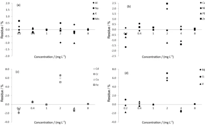
was done in relation to the experimental values (Figure 1). Figure 1 indicates that the residues were mostly less than ± 2%, only a few exceeded this value, however, they did not exceed 10%, indicating that the 2nd order polynomial
regression is a good representation of the concentrations found in the standard addition curve. Therefore, it can be concluded that although the sample filter of the atmospheric particulate matter (sample matrix) contains in its composition many of analytes present in the sample, they do not interfere with the analytical signal of interest.
Figure 1. Residue of (a) Al, K, Mn and Na; (b) Ca, Zn, Ni and Pb; (c) Cd, Cu, Cr and Fe and (d) Mg, Ti and V obtained of the 2nd order polynomial
The second evaluation of selectivity was done to assess if there was any interference of the matrix in the analytic results of the particulate matter. A t-student test (Table S4, Supplementary Information) was done using results of the differences into metal concentrations of dilutions of the matrix with and absent addition of standard solution.
As the concentrations results obtained for several dilutions revealed to be equivalent for all investigated elements, it can be concluded that the dilution of the matrix does not influence the analytical response. Therefore, it is not necessary to dilute the sample of particulate matter to dilute the matrix. Thus, the manner in which the sample was used for the determination of metals by Gioda et al.24 was
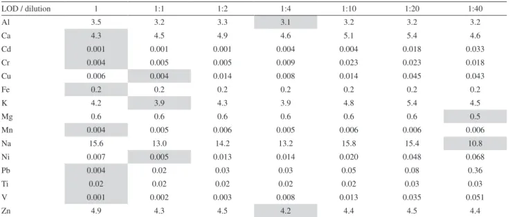
sufficiently adequate. A procedure to select which optimum dilution of the matrix should be adopted for the determination of metals in particulate matter by ICP-OES is by observing the limits of detection of each dilution as shown in Table 1.
The lower limits of detection for each of the analyzed metals with the different dilutions of the matrix are highlighted in gray in Table 1.
It can be concluded that the way in which the acidic solution from the extraction of particulate matter by Gioda et al.24 for the determination of metals by ICP-OES
(without dilution of the matrix) was the best procedure that could have been adopted as, for most metals when dilution was not made, a lower limit of detection was obtained.
Linearity
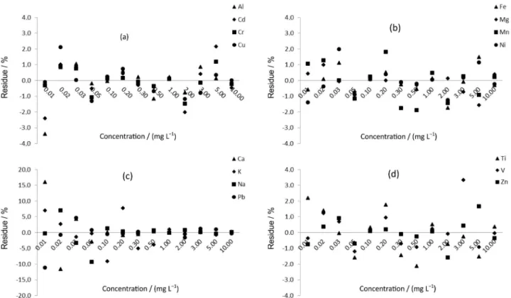
To evaluate the linearity, three external calibration curves were prepared: 0.01 to 0.1 (1), 0.2 to 1.0 (2), 2.0 to 10.0 (3) mg L-1 of multielement standard solution. The
heteroscedasticity was evaluated through the residue graph (Figure 2) in relation to the linear regression. Extremely high residues were observed with an average of 133% when a single curve was used for this range of concentration. However, when the residues were checked using a curve for low concentrations (0.01-0.1 mg L−1), another curve
for medium concentrations (0.2-1.0 mg L−1) and one for
high concentrations (2.0-10.0 mg L−1) the residues were to
± 2% (Figure 2). Only calcium and lead obtained a residue greater to 10%.
Table S5 (Supplementary Information) shows the Pearson coefficients of low, medium and high concentration curves when done the linear regressions following the of least squares method of the analyte concentration versus the emission intensity.
According to Green32 and Shabir,33 correlation
coefficients values higher than 0.999 is the evidence of an optimal fit of the data for the regression line. However, the curves were quite linear for all elements in the concentrations evaluated, with the exception of the elements K and Na, which only showed a correlation coefficient upper to 0.999 after the concentration of 1.0 and 0.1 mg L−1, respectively.All correlation coefficient
values of K and Na were higher than that recommended by ANVISA15 (r ≥ 0.99) and the required by INMETRO13
(r ≥ 0.90), considering that the curve is linear.
Limit of detection and quantification
The limits of detection and quantification shown in Table 2 were determined with the matrix solution. The limits of detection were inferior to 0.02 mg L−1 for most of the
Table 1. Limit of detection (mg L−1) in several dilutions of the matrix
LOD / dilution 1 1:1 1:2 1:4 1:10 1:20 1:40
Al 3.5 3.2 3.3 3.1 3.2 3.2 3.2
Ca 4.3 4.5 4.9 4.6 5.1 5.4 4.6
Cd 0.001 0.001 0.001 0.004 0.004 0.018 0.033
Cr 0.004 0.005 0.005 0.009 0.023 0.023 0.018
Cu 0.006 0.004 0.014 0.008 0.014 0.045 0.043
Fe 0.2 0.2 0.2 0.2 0.2 0.2 0.2
K 4.2 3.9 4.3 3.9 4.8 5.4 4.5
Mg 0.6 0.6 0.6 0.6 0.6 0.6 0.5
Mn 0.004 0.005 0.006 0.005 0.006 0.006 0.006
Na 15.6 13.0 14.2 13.2 15.8 15.4 10.8
Ni 0.007 0.005 0.013 0.014 0.020 0.048 0.068
Pb 0.004 0.02 0.03 0.03 0.05 0.08 0.36
Ti 0.02 0.02 0.02 0.02 0.02 0.03 0.03
V 0.001 0.002 0.003 0.008 0.013 0.035 0.051
metals with the exception of Al, Ca, Fe, K, Mg, Na e Zn that remained in the range of 0.1 a 16.0 mg L−1 as they are already
present in significant concentrations in the blank filter. Regarding the detection limits described in U.S. EPA Method IO-3.4 for metals that are not heavily present in the matrix of the sample, very close values can be observed (Table 3).
Recovery
To evaluate the recovery (Table 4) of the method of extraction, solutions with SRM1648a were prepared with 10 mg, to ensure the homogeneity of the sample and to approach the mass of the sampled atmospheric particulate matter.
Once the recovery of the method is known, it can be used and the recovery factor can be applied to the results to know the total concentration of all analytes present in the samples of particulate matter.
Accuracy
The accuracy was obtained by the evaluation of standard solution for four concentrations belonging to the working range: 0.2, 0.5, 1.0 and 5.0 mg L−1, added to the matrix
solution. The relative error was calculated in relation to the experimental results and the expected results (Table 5).
The relative errors varied from 0.2 to 10% for all elements. Therefore, they are below the maximum
recommended by ANVISA15 (15%).
Repeatability
The repeatability of the method was examined for a range of multi-element standard solution of concentrations 0.2,
Figure 2. Residues obtained of (a) Al, Cd, Cu and Cr; (b) Fe, Mg, Mn and Ni; (c) Ca, K, Na and Pb and (d) Ti, V and Zn by using 3 external calibration curves.
Table 2. Limits of detection and operational quantification (mg L−1) for
ICP-OES
Element Average deviationStandard detectionLimit of quantificationLimit of
Al 3.44 0.01 3.47 3.55
Ca 4.23 0.03 4.33 4.56
Cd 0.0008 0.0001 0.0011 0.0018
Cr 0.0029 0.0005 0.0044 0.0079
Cu 0.0046 0.0004 0.0058 0.0086
Fe 0.1532 0.0006 0.1550 0.1592
K 4.09 0.05 4.24 4.60
Mg 0.60 0.05 0.62 0.65
Mn 0.0038 0.0001 0.0041 0.0048
Na 15.25 0.13 15.64 16.53
Ni 0.0045 0.0008 0.0069 0.0125
Pb 0.0032 0.0002 0.0038 0.0052
Ti 0.0166 0.0001 0.0169 0.0176
V 0.0006 0.0003 0.0015 0.0036
0.5, 1.0, 2.0 and 10.0 mg L−1 that were added to the matrix
solution. The results of the relative standard deviation for each of the 15 elements determined are shown in Table 6.
Intermediate precision
Intermediate precision was evaluated on the same sample used to evaluate the repeatability, using the same method in the same laboratory, but in different days and with different analysts. Table S6 (Supplementary Information) presents the RSD of intermediate precision at different concentrations of analytes.
According to Huber,21 the methods used to quantify the
analyte with maximum of 10 mg L–1 has an acceptable RSD
lower or equal to 7.3% and for analytes of 1 mg L−1 lower or
equal to 11%, depending on the complexity of the sample.
On the other hand, ANVISA15 establishes the maximum as
15%. Therefore, the relative standard deviations observed in the analysis of repeatability and intermediate precision are satisfactory for the concentration range examined, as they were always inferior to 5%.
Comparison of the precisions and recoveries of extraction methods
After determining the concentrations of the analytes of two extraction methods, U.S. EPA IO-3.111 and our
Table 3. Limits of detection (mg L−1) of our method and U.S. EPA
IO-3.4 method9
Element Spectral lines Our method U.S. EPA
Cd 214.440 0.001 0.005
Cr 267.716 0.004 0.012
Cu 327.393 0.006 0.01
Mn 257.610 0.004 0.004
Ni 231.604 0.007 0.014
Pb 220.353 0.004 0.032
Ti 334.940 0.017 0.003
V 292.402 0.002 0.007
Table 4. Analytical recovery with SRM 1648a
Element Our method / (mg kg−1)
SRM 1648ª / (mg kg−1)
Recovery / %
Al 5893 34300 17
Ca 59458 58400 99
Cd 60.8 73.7 83
Cr 66 402 16
Cu 568 610 93
Fe 22629 39200 58
K 3126 10560 30
Mg 5585 8130 69
Mn 638 790 81
Na 1638 4240 39
Ni 55.2 81.1 68
Pb 6151 6550 94
Ti 273 4021 7
V 81 127 64
Zn 3969 4800 83
Table 5. Relative errors (%) per range of analyte concentration
Element Concentration / (mg L
−1)
0.2 0.5 1.0 5.0
Al 5.9% 5.1% 0.3% 2.3%
Ca 0.3% 3.1% 1.4% 0.6%
Cd 6.2% 5.8% 0.3% 6.1%
Cr 5.5% 5.4% 0.5% 3.6%
Cu 5.0% 4.7% 0.8% 1.0%
Fe 4.0% 4.4% 9.7% 4.9%
K 6.7% 9.9% 7.2% 5.9%
Mg 7.0% 6.4% 0.4% 3.1%
Mn 5.1% 5.0% 0.6% 4.1%
Na 0.7% 1.2% 1.4% 0.6%
Ni 5.0% 5.3% 0.4% 1.4%
Pb 4.9% 5.2% 0.6% 1.9%
Ti 5.0% 4.8% 1.1% 2.0%
V 6.2% 5.2% 0.7% 3.2%
Table 6. Relative standard deviation (%) in different analyte concentrations
Element Concentration of the standard solution / (mg L
−1)
0.2 0.5 1.0 2.0 10.0
Al 0.79 1.14 0.42 0.40 1.62
Ca 0.59 0.91 0.30 0.85 1.23
Cd 0.86 1.60 0.53 0.40 2.95
Cr 0.60 1.29 0.52 0.41 2.97
Cu 0.58 1.14 0.53 0.49 3.00
Fe 0.74 1.30 0.47 0.41 2.86
K 0.85 0.81 0.51 0.93 1.14
Mg 0.74 0.94 0.29 0.94 1.65
Mn 0.73 1.29 0.19 0.25 2.98
Na 0.72 0.88 0.37 0.83 0.79
Ni 0.73 1.36 0.52 0.41 2.52
Pb 1.40 1.62 0.62 0.34 2.24
Ti 0.41 1.11 0.22 0.32 3.04
V 0.78 1.19 0.56 0.44 2.99
method, with duplicated samples (n = 2), for the same mass of certified reference material SRM 1648A (m = 10 mg), by the same method of determination (ICP-OES) under the same analytical conditions, the analyses of the differences of efficiencies of extraction (recovery) (Table 7) and an F-test (precision) were done to assess if there is any equivalence between the methods (Table 14).
The recoveries are very similar, not differing by 5% for most metals. This value was only exceeded for Cd, Fe and Mn, it however, did not exceed 15%.
It is important to remark that as our as U.S. EPA IO-3.1 methodologies only determine the metals soluble in HNO3,
excluding the fraction of metals binding to silicates. The results of the F-test indicated that the two extraction methods have equivalent precisions (Table 8). Therefore, the method adopted in our lab is quite similar to U.S. EPA method IO-3.1, which is the most common method for the determination of metals in atmospheric particulate material.
Robustness
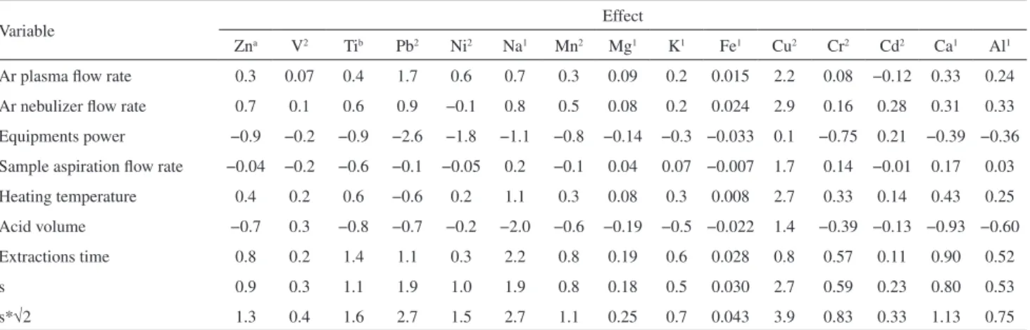
Comparing the results of the effects of each variable to the standard deviation of 8 samples multiplied by the square root of two (√2 s) it was impossible to evaluate whether the values of the effects were significant and therefore alter the analytical response (Table 9) .
Applying the Youden and Steiner test,30 it can be
concluded that only Ni may suffer variations in its analytical response if the power of the equipment varies from 500 W
to 400 W, which is not expected during the analysis due to the stability of the plasma in this equipment. Therefore, we can conclude that the method is robust for all variables found in the considered experimental domain.
Conclusion
Among the analyzed elements, Al, Na, K, Ca and Zn are strongly present in the matrix of the sample. However, through tests of selectivity, it can be observed
Table 7. Analysis of recoveries of extraction methods
Element Our method U.S. EPA IO-3.1 Difference / %
Al 17.8 17.1 −0.7
Ca 101.1 101.8 0.7
Cd 89.5 82.5 −7.0
Cr 17.9 16.5 −1.4
Cu 95.8 93.2 −2.6
Fe 71.8 57.7 −14.0
K 30.4 29.6 −0.8
Mg 68.8 68.7 −0.1
Mn 87.9 80.8 −7.1
Na 41.5 38.7 −2.9
Ni 72.6 68.0 −4.5
Pb 93.6 93.9 0.3
Ti 9.9 6.9 −3.0
V 66.3 64.1 −2.2
Zn 85.2 82.7 −2.5
Table 8. Equivalence test between the precision of the extraction methods
Element Standard deviation U.S. EPA IO-3.1 Standard deviation Our method Calculated F Critic F Result
Al 0.0081 0.011 0.54 4.28 same
Ca 0.0017 0.0009 3.79 – same
Cd 0.12 0.11 1.40 – same
Cr 0.0002 0.0002 0.69 – same
Cu 0.0005 0.0003 2.51 – same
Fe 0.0011 0.0009 1.56 – same
K 0.050 0.044 1.30 – same
Mg 0.008 0.015 0.34 – same
Mn 0.013 0.010 1.87 – same
Na 0.0011 0.0010 1.12 – same
Ni 0.0054 0.0044 1.49 – same
Pb 0.0008 0.0006 1.62 – same
Ti 0.0093 0.011 0.72 – same
V 0.006 0.041 0.02 – same
that this did not influence the analytical response of other metals analyzed. Furthermore, by linearity test it can be concluded that the working range adopted for the measurement of concentrations of metals in atmospheric particulate matter is linear and with random and small residues. Finally, the method of extraction of metals from PM adopted by our lab shows good precision and accuracy, and it is equivalent to the standard method (U.S. EPA IO-3.1). The developed method may be used to determine Al, Ca, Cd, Cu, Cr, Fe, K, Mg, Mn, Na, Ni, Pb, Ti, V and Zn present in atmospheric particulate matter (PM2.5) by ICP-OES, because it meets all validation requirements set by INMETRO.
Supplementary Information
Supplementary data are available free of charge at http://jbcs.sbq.org.br as PDF file.
Acknowledgements
The authors are grateful to the Environment Institute of Rio de Janeiro State (INEA) for providing PM2.5 samples
and filters; and for Foundation Agencies Support Research in Rio de Janeiro State (FAPERJ), National Council for Technological and Scientific Development (CNPq) and Brazilian Federal Agency for Support and Evaluation of Graduate Education (CAPES) for financial support for the research.
References
1. Environment National Consul (CONAMA); Padrões Nacionais da Qualidade do ar, Resolução CONAMA Nº 03: DF, 1990. 2. Smith, I. M.; Trace Elements from Coal Combustion
Emissions, IEA Coal Research: London, 1987.
3. Baird, C.; Química Ambiental, Bookman: Porto Alegre, 2002. 4. World Health Organization (WHO); Health Aspects of Air
Pollution with particulate Matter, ozone and Nitrogen Dioxide; Report on a WHO Working Group: Bonn, 2003.
5. Mohanraj, R.; Azeez, P. A.; Priscilla, T.; Arch. Environ. Contam. Toxicol. 2004, 47, 162.
6. Arbilla, G.; Maia, L. F. P. G.; Quiterio, S. L.; Escaleira, V.; Sousa, C. R. S.; Bull. Environ. Contam. Toxicol. 2004, 72, 916. 7. Gontijo, E. S. J.; Oliveira, F. S. D.; Fernandes, M. L.; Silva, G. A.; Roeser, H. M. P.; Friese, K.; J. Braz. Chem. Soc. 2014, 25, 208. 8. Carvalho, F. G.; Jablonski, A.; Teixeira, E. C.; Quim. Nova
2000, 23, 614.
9. US Environmental Protection Agency (U.S. EPA); Method IO-3.4: Determination of metals in ambient particulate matter using ICP-OES; Washington, 1999.
10. Soluri, D. S.; Godoy, M. L. D. P.; Godoy, J. M.; Roldão, L. A.; J. Braz. Chem. Soc. 2007, 18, 838.
11. US Environmental Protection Agency (U.S. EPA); Method IO-3.1: Selection, Preparation and extraction of filter material; Washington, 1999.
12. Ribani, M.; Bottoli, C. B. G.; Collins, C. H.; Jardim, I. C. S. F.; Melo, L. F. C.; Quim. Nova 2004, 27, 771.
13. National Institute of Metrology, Standard and Industrial Quality (INMETRO); Orientações sobre Validação de Métodos de Ensaios Químicos; 4th rev.; DOQ-CGCRE-008: Rio de Janeiro, 2011.
14. World Health Organization (WHO); Expert Committee on Specifications for Pharmaceutical Preparations, 32nd report;
WHO Technical Report Series: Geneva, 1992.
15. National Health Surveillance Agency (ANVISA); Guia para Validação de Métodos Analíticos e Bioanalíticos; Resolução nº 899: Brasília, 2003.
16. International Conference on Harmonisation (ICH); Guidance for Industry-Q2B Validation of Analytical Procedures: Methodology; London, 1996.
Table 9. Effect values obtained by Youden and Steiner test30
Variable Effect
Zna V2 Tib Pb2 Ni2 Na1 Mn2 Mg1 K1 Fe1 Cu2 Cr2 Cd2 Ca1 Al1
Ar plasma flow rate 0.3 0.07 0.4 1.7 0.6 0.7 0.3 0.09 0.2 0.015 2.2 0.08 −0.12 0.33 0.24
Ar nebulizer flow rate 0.7 0.1 0.6 0.9 −0.1 0.8 0.5 0.08 0.2 0.024 2.9 0.16 0.28 0.31 0.33 Equipments power −0.9 −0.2 −0.9 −2.6 −1.8 −1.1 −0.8 −0.14 −0.3 −0.033 0.1 −0.75 0.21 −0.39 −0.36 Sample aspiration flow rate −0.04 −0.2 −0.6 −0.1 −0.05 0.2 −0.1 0.04 0.07 −0.007 1.7 0.14 −0.01 0.17 0.03
Heating temperature 0.4 0.2 0.6 −0.6 0.2 1.1 0.3 0.08 0.3 0.008 2.7 0.33 0.14 0.43 0.25 Acid volume −0.7 0.3 −0.8 −0.7 −0.2 −2.0 −0.6 −0.19 −0.5 −0.022 1.4 −0.39 −0.13 −0.93 −0.60
Extractions time 0.8 0.2 1.4 1.1 0.3 2.2 0.8 0.19 0.6 0.028 0.8 0.57 0.11 0.90 0.52
s 0.9 0.3 1.1 1.9 1.0 1.9 0.8 0.18 0.5 0.030 2.7 0.59 0.23 0.80 0.53
s*√2 1.3 0.4 1.6 2.7 1.5 2.7 1.1 0.25 0.7 0.043 3.9 0.83 0.33 1.13 0.75
17. Thompson, M.; Ellison, S. L. R.; Wood, R.; Pure Appl. Chem.
2002, 74, 835.
18. International Standard Organization (ISO); General Requirements for the Competence of Testing and Calibration Laboratories; ISO/IEC 17025, 1999.
19. United States Food and Drug Administration (US-FDA), Center for Drug Evaluation and Research (CDER); General Principles of Validation; Rockville, 1987.
20. United States Pharmacopeia Convention; US Pharmacopeia 24; Validation of Compendial Methods, Rockville, 1999. 21. Huber, L.; LC-GC Int. 2001, 11, 96.
22. Jenke, D. R.; Instrum. Sci. Technol. 1998, 26, 1.
23. Bruce, P.; Minkkinen, P.; Riekkola, M. L.; Mikrochim. Acta
1998, 128, 93.
24. Gioda, A.; Amaral, B. S.; Monteiro, I. L. G.; Saint’pierre, T. D.; J. Environ. Monit. 2011, 13, 2134.
25. Ribeiro, F. A. L.; Ferreira, M. M. C.; Quim. Nova 2008, 31, 164.
26. Vessman, J.; Stefan, R. I.; Van Staden, J. F.; Danzer, K.; Lindner, W.; Burns, D. T.; Fajgelj, A.; Müller, H.; Pure Appl. Chem. 2001,
73, 1381.
27. Guilhen, S. N.; Pires, M. A. F.; Keiko, E. S.; Xavier, D. F. B.; Quim. Nova 2010, 33, 1285.
28. National Institute Standards and Technology (NIST); Certificate Analysis of Standard Reference Material 1648ª (Urban Particulate Matter), USA, Gaithersburg, 2008.
29. Leite, F.; Validação em Análise Química, 4th ed.; Átomo:
Campinas, 2002.
30. Youden, W. J.; Steiner, E. H.; Statistical Manual of the AOAC, 48th ed.; AOAC International: Arlington, 1975.
31. Brito, N. M.; Amarante Junior, O. P.; Polese, L.; Ribeiro, M. L.; Pesticidas: r. ecotox. meio ambiente 2003, 13, 129.
32. Green, J. M.; Anal. Chem. 1996, 68, 305. 33. Shabir, G. A.; J. Chromatogr. A 2003, 57, 987.
Submitted on: April 6, 2014