doi: 10.1590/0101-7438.2017.037.02.0277
EXPLORING THE CO-AUTHORSHIP NETWORK AMONG CNPQ’S PRODUCTIVITY FELLOWS IN THE AREA OF INDUSTRIAL ENGINEERING
Ricardo Lopes de Andrade
1*and Leandro Chaves Rˆego
2Received August 16, 2016 / Accepted June 22, 2017
ABSTRACT.In this article, we have built a co-authorship network among researchers with CNPQ grant in research productivity (PQ) in the area of Industrial Engineering and analyze which Social Network Analysis metrics impact their productivity level. Unlike other studies that mostly analyze unweighted networks, ours explored more broadly the network since the metrics were calculated in three ways: unweighted, including the edges weights and including the edges and nodes’ attributes. Thus, the generated results are more precise and detailed since more information is obtained. We consider theh-index of the researchers as the nodes’ attributes and measured the impact using Kendall correlation. We show that geographical distance is still a barrier to collaboration among PQs in this area and that collaboration with researchers with different levels of grant has the greatest impact in the level of the grant a researcher has.
Keywords: weighted co-authorship network, nodes’ attributes, scientific productivity.
1 INTRODUCTION
Co-authorship, development of a publication by two or more authors, is a form of collaboration. For Hudson (1996), co-authorship is the most formal expression of intellectual collaboration in scientific research, and the biggest gain of the collaboration is to enable an efficient task division, through the complementary skills or synergy (joint creation of new ideas, not achieved individually). The result of this efficient task division is a scientific production of higher quality and/or quantity. These results had already been reported by Barnett et al. (1988) as the reason that leads researchers to work together. Other works, such as Eaton et al. (1999) and Lee & Bozeman (2005), also point productivity as a result of collaboration. Hart (2000) shows that collaboration improves the quality of publications.
*Corresponding author.
1Universidade Federal de Pernambuco. Programa de P´os-Graduac¸˜ao em Engenharia de Produc¸˜ao, Avenida da Arquite-tura, 50740-550 Recife, PE, Brasil. E-mail: [email protected]
Co-authoring, writing the same paper with other authors, is a form of collaboration which implies a temporal and academic relationship, where authors share ideas and resources. One of the most famous co-authorship networks is the mathematician Paul Erdos network, which has more than 500 co-authors and more than 1,400 published works. The role of Erdos as a collaborator was so significant in the field of mathematics that the Erdos number is set to measure the proximity to Erdos through network co-authorship (Liu et al., 2014). Anyone who has published with Erdos has an Erdos number equal to 1, those having a publication with a co-author Erdos have an Erdos number equal to 2, and so on (Newman, 2001c).
For Kumar (2015), studies on co-authorship gained new interest after Newman (2001a, b, c, 2004) have used methods of social network analysis to investigate the characteristics and interest-ing patterns of academic communities. Kempe & Kleinberg (2005) also reported the emergence of many researches of co-authorship network analysis that try to identify the most influential au-thors in it. It is also observed that the works of Huang et al. (2013) and Liu et al. (2014) sought to study the co-authorship network to assess the status of an author in a particular field, and thus enhance the relations to get closer to the community core by identifying the most influential researchers.
There exists an increasing interest in the study of the influence of the social structure on the behavior and performance of the researchers through social network analysis (SNA). Many of these studies seek to correlate the key centrality metrics of the network with measures based on the number of citations, such as theh-index (“A researcher has ah-index ofk, ifkofNhis works have at leastkcitations each, and the other (N−k) papers have at mostkcitations each”, Hirsch, 2005). Such measures, among other factors, can be used to determine the quality of publications.
The work of Yan & Ding (2009) correlated four centrality metrics (degree, closeness, between-ness and PageRank) with the number of citations of publications of the authors of a co-authorship network. These metrics had significant correlations with the citation counts, especially the betweenness centrality.
Another work that also correlates analytical metrics of social networking with theh-index was published by Wanderley et al. (2014). The authors created a co-authorship network among re-searchers of Computer Science and calculated normalized metrics of degree centrality, closeness centrality, and betweenness centrality, weighted degree centrality and authority (calculated by adding the number of hubs, nodes with many links, with which a node is connected). Only the betweenness centrality and the weighted degree centrality had significant positive correlations. The authority also showed significant, but negative correlation.
Souza et al. (2016), in a co-authorship network among researchers with CNPq grant in research productivity in the area of Statistics, showed that the most productive fellows are also the most central in the network and that the metrics degree centrality and closeness centrality had a higher impact on the number of articles published by a fellow.
According to CNPq (2015), the research productivity fellowship (PQ) is organized in levels, in ascending order: 2, 1D, 1C, 1B, 1A. The PQ is attributed to researchers from all areas of knowledge in Brazil, based not only on the quality of a submitted project, but mainly in the “quality” of the researcher (Wainer & Vieira, 2013).
The work of Fonseca & Digiampietri (2016) builds two kinds of classifiers using as attributes considering SNA metrics and other bibliometric measures. The first kind identifies among re-searchers in the area of Computer Science who are the fellowships holders and the other kind identifies the fellowship level of a given researcher. Other studies analyzing the impact of the co-authorship networks in the performance of the researchers were presented in Andrade & Rˆego (2015a, 2015b).
In these previous works, weighted metrics were not used, i.e., metrics calculated considering the frequency of the collaboration, with the exception of the weighted degree centrality. To the best of our knowledge, there are few works exploring such metrics in SNA. Liu et al. (2015) proposed a method that inserts the importance (based on citations) of researchers in co-authorship network structures redefining the weight of the edges. This weight is used in the calculation of PageRank, applied to the Erdos network, to identify the most influential authors. Andrade (2016) also developed a metric that inserts the importance of nodes in the network structure, in this work, the weight of a given edge is equal to the average of the nodes’ attributes connected by this edge times the original weight of the edge. This work has addressed the impact of the nodes’ attributes in different SNA metrics.
The objective of this work is to identify the researchers with the CNPq grant in research pro-ductivity in the area of Industrial Engineering in Brazil, to analyze their academic achievements in terms of published papers, to construct a co-authorship network among such researchers, to analyze the characteristics of the network and to verify which SNA metrics have more impact in their productivity level. SNA metrics will be calculated in three ways: unweighted, weighted with the weight the edges and weighted with weights of the edges and the nodes’ attributes.
nodes’ attributes are taken into consideration. Theh-factor is a node attribute which was freely available to use and is clearly related to the prestige of some researcher. Therefore, it was chosen to be applied in this context.
The structure of this work is divided as follows: in this first section we present a review of the studies that analyzed the influence of the SNA metrics, co-authorship networks and the perfor-mance of the researchers; Section 2 briefly presents the SNA metrics used in this work; Section 3 describes the methodology used to create the co-authorship network; the co-authorship network and the impact of individual SNA metrics on the level of productivity is presented in Section 4. Finally, Section 5 presents the final considerations of the study and proposals for future work.
2 SOCIAL NETWORK ANALYSIS METRICS
A weighted network can be defined as a set of nodes,V(G), a set of edges,E(G), which consists of ordered pairs of nodes, and a weighted adjacency matrix,W(G), wherew(vi, vj)represents the weight associated with the edge connecting the pair of vertices,vi andvj. We assume that w(vi, vj)=w(vj, vi), since co-authorship is a symmetric relation.
Liu et al. (2015) and Andrade (2016) developed methods to include nodes’ attributes in the SNA. Thus, it is possible to classify networks as unweighted, weigthed by edges and weighted by edges and nodes. Since Liu et al.’s method transform the network into an asymmetric relation, we do not view it as appropriate to study co-authorship. Therefore, we focus here on Andrade’s method which mantains the symmetric nature of co-authorships.
The metric proposed by Andrade (2016) as a way to take into consideration the importance of the node in the network context is given by:
Z(vi, vj)=w(vi, vj)× s(v
i)+s(vj)
2
, (1)
whereZ(vi, vj)equals the edge weightw(vi, vj)between verticesviandvj, combined with the
attributes of these verticess(vi)ands(vj), respectively. With the incorporation of the attributes
of the nodes in the network, Z(G)shall be the new weighted adjacency matrix and Z(vi, vj)
the new edge weight between verticesvi andvj. The attributes of the vertices are measurable
characteristics associated with the type of relationship that connects them.
A binary network with n vertices is represented by an adjacency matrixA(G)withn×nelements, where
a(vi, vj)=
1 if(vi, vj)∈ E(G), i.e. ifvi andvj are connected,
0 otherwise. (2)
The SNA metrics can be divided intoglobal, describing the characteristics of the whole graph, andindividual, which are related to the analysis of individual properties of network actors (nodes or vertices).
Apathbetween two vertices,vi andvj, is a sequence of verticesc=(v0, v1, v2, . . . , vk)such
thatv0 = vi,vk = vj,vl is adjacent tov(l+1), forl = 0,1, . . . ,k−1 and there is no pair of vertices that appear more than once in the sequence. A set of vertices is said to beconnectedif there exists a path between any two vertices in the set. A graph isconnectedif there is a path between any two vertices and iscompleteif every vertice is connected to one another.
Thedensitycalculates how close the graph is to being complete. That is, the relationship between total connections in the graph and the total connections if all vertices were connected to each other. For an undirected graph withnnodes, the density is defined as:
Dens(G)=2×(#E(G))
n×(n−1) (3)
Ageodesic pathor shortest path is the shortest path between two vertices, Newman (2004). The geodesic path length,d(vi, vj), also calledgeodesic distance or shortest distance, thus, is the
shortest distance in the network between these two vertices. Given a pathc=(v0, v1, v2, . . . , vk)
between verticesvi andvj, the length of this path is given bydc. LetC(vi, vj)be the set of all
paths between verticesvi andvj, then the geodesic distance is defined by:
d(vi, vj)=mindc:c∈C(vi, vj). (4)
In the case of weighted networks, the length of a pathc=(v0, v1, v2, . . . , vk)between vertices
vi andvj, can be formally defined by Dijkstras algorithm Newman (2001) and Brandes (2001):
dcw =
1
w(v0, v1)
+ 1
w(v1, v2)
+ · · · + 1
w(v(k−1), vk)
. (5)
And the weighted geodesic distance is given by:
dw(v1, v2)=mindcw:c∈C(vi, vj)
. (6)
The largest geodesic distance between any pair of vertices is called thediameterof a graph and in a binary network, it can vary from a minimum of 1, if the graph is complete, to a maximum of n−1, where n is the number of vertices in the graph. Formally, the diameter of the connected graphGis given by:
Dim(G)= max
{vi,vj∈V(G)}
d(vi, vj) (7)
In case of weighted networks, the weighted diameter is calculated using the weighted geodesic distance,dw(vi, vj).
Also known as the giant component, the size of thelargest connectedcomponent, refers to the cardinality of the connected component with the highest number of nodes.
Given a vertexvi,eccentricity,e(vi), is the maximum distance from it to any other vertex of the graph. The relationship of a vertex to other vertices is better the smaller the eccentricity. Thevi
eccentricity is given by:
e(vi)= max vj∈V(G)
The diameter, as defined above, is equal to the maximum eccentricity, while the minimum eccen-tricity is theradius. In the case of weighted networks, the eccentricity may be calculated using the weighted geodesic distance,dw(vi, vj).
The degree centrality, proposed by Freeman (1979), is calculated in terms of the number of adjacent vertices, namely, degree centrality of the vertexvi, denoted byCd(vi)is the number of
vertices adjacent to vertexvi. Formally the degree centrality is defined by:
Cd(vi)=
n
j=1
a(vi, vj) (9)
If the network is weighted, the degree centrality of vertexvi is equal to the sum of the weights of the edges that are connected to the vertexvi. For Newman (2004) and Barrat et al. (2004) the
weighted degree centrality is defined by:
Cdw(vi)=
n
j=1
w(vi, vj). (10)
The degree centrality is the simplest and easiest way to measure the influence of a node (Abbasi et al., 2012; Liu et al., 2005). In a co-authorship network, this metric identifies the most active and popular authors (Abbasi et al., 2011; Anastasios et al., 2012; Freeman, 1979).
Another metric to analyze a node on the network started from the theory of “the strong links” of Krackhardt (1992). Theaverage link strengthof vertexvi is defined as the ration between the weighted degree,Cdw(vi), and the degree centrality,Cd(vi):
L S(i)=C w
d(vi)
Cd(vi) (11)
Therefore, L S(i)represents the average weight of the links of nodevi.
A metric that takes into consideration the geodesic distance from a given initial node to all other nodes of the network is thecloseness centrality. Freeman (1978) asserted that the closeness centrality of vertexvi, defined byCc(vi), is given by:
Cc(vi)= 1
jd(vi, vj)
(12)
The most central vertices in a network according to this metric are those that have a smaller distance to the other vertices. In weighted networks, the weighted closeness centrality is given by:
Ccw(vi)=
1
jdw(vi, vj)
(13)
Thebetweenness centralityof vertexvi is the sum, for every pair of nodes different fromvi, of
the ratio between the number of shortest paths between the given pair of nodes that go through
vi, and the total number of shortest paths between the given pair of nodes (Freeman, 1979;
Wasserman & Faust, 1994). The betweenness centrality,Cb(vi), of vertexviis given by:
Cb(vi)=
j,k
g(vj, vi, vk)
g(vj, vk)
, j=k=i, (14)
whereg(vj, vk)is the number of shortest paths between vertexvj and vertexvkandg(vj, vi, vk)
is the number of shortest paths between vertexvj and vertexvkgoing throughvi.
In a weighted network the betweenness centrality is given by:
Cbw(vi)=
j,k
gw(vj, vi, vk)
gw(v
j, vk)
, (15)
wheregw(vj, vk)is the number of weighted shortest paths between vertexvj and vertexvk and
gw(vj, vi, vk)is the number of weighted shortest paths between vertexv
j and vertexvk going
throughvi, considering the weighted distance,dw(vi, vj).
The betweenness is an indicator of the potential of a node to play the role of “mediator” or “gatekeeper” (Freeman, 1979; Abbasi et al., 2012), being able to control more often the flow of information on the network.
A metric of importance of the vertex in the network based on the connections, theeigenvector centralityis supported on the idea that a particular node will have high centrality if it is connected to vertices with central positions in the network (Bonacich, 1987). In other words, the centrality of the vertex does not depend only on the number of adjacent vertices but also on the centrality of these vertices. Letλbe a constant, then the eigenvector centrality ofCe(vi)is given by:
Ce(vi)=
1
λ n
j=1
a(vi, vj)Ce(vj) (16)
Using the vector notation, letX =(Ce(1),Ce(2) . . .Ce(n))be the vector of eigenvector
central-ities, we can rewrite Equation (14) asλX = AX. By assuming that the eigenvector centrality assumes only non-negative values (using the Perron-Frobenius theorem), it can be shown that
λis the largest eigenvalue of the adjacency matrix, where X is the corresponding eigenvector (Jackson, 2008).
In the case of weighted networks, the elements of the adjacency matrix are the weights of the edges,w(vi, vj), (Newman, 2004). And the eigenvector centrality is defined by:
Cew(vi)= 1
λ n
j=1
w(vi, vj)Cew(vj) (17)
(networks with large cluster coefficient and the relatively short distance between the nodes), Watts & Strogatz (1998). The clustering coefficient of a vertex vi is the ratio of the number of triangles that contains vertex vi and the number of possible edges between the neighboring
vertices. LetN T(vi)be the number of triangles (consists of three nodes connected by three links) containing vertexvi. For Onnela et al. (2005), the local cluster coefficient is defined as:
CC L(vi)=
2N T(vi)
Cd(vi)(Cd(vi)−1)
(18)
The weighted local clustering coefficient was proposed by Onnela et al. (2005) and is given by:
CC Lw(vi)=
2
Cd(vi)(Cd(vi)−1)
j,k
ˆ
w(vi, vj)w(vˆ i, vk)w(vˆ j, vk)
1/3
, (19)
where the weights of the edges are normalized by the maximum weight of the network,
ˆ
w(vi, vj) = w(vi, vj)maxi,j∈V(G)(w(vi, vj)) and the contribution of each triangle depends on all the weights of the edges.
The average clustering coefficient is the average value of the individual or local coefficients and is given by:
C L(G)= 1 n
i
CC L(vi) (20)
The clustering coefficient, C L(G), for the co-authorship network refers to the probability that any two collaborators of a researcher have collaborated with each other (Onel et al., 2011). In the individual case, the clustering coefficient of a particular author indicates how his collaborators are working together.
PageRankis a method of ranking web pages, measuring effectively the interest of browsers and attention devoted to them, Page at al. (1999). The PageRank considers the number and quality of links to a web page in order to determine how influential it is (Liu et al., 2014). LetTAbe a web
page andTione of the web pages that connects toTA. Brin & Page (1998) defined PageRank as
follows:
P R(TA)=(1−δ)+δ
P R(T 1)
C(T1)
+ · · · + P R(Tn) C(Tn)
, (21)
where P R(TA)is the PageRank of pageTA, P R(Ti)is the PageRank of pageTi,C(Ti)is the
number of outbound links on pageTi andδis a damping factor (assuming that a person randomly
clicks on pages and eventually stops clicking,δis the probability at any given moment, the person will continue to click), which can be set between 0 and 1.
is given by the product of the dedication of each author to the collaboration. Formally, a utility Uw(vi)of a given authorvi in a given graphGis given by:
Uw(vi)=
j
w(vi, vj)
Cwd(vi)
+w(vi, vj) Cdw(vj)
+ w(vi, vj)
2
Cdw(vi)Cdw(vj)
, (22)
wherew(vi, vj)is the total number of works between authorsvi andvj,Cwd(vi)andCdw(vj)
are the weighted degrees of these authors, respectively.
The utility developed by Santos (2014) was based on the original model of the utility of Jackson & Wolinsky (1996). This model takes into account only if the author is or is not connected to another author, disregarding the number of works done together. Thus the utility of a particular authorvi in a given graphGis given by:
U(vi)=
j
1 Cd(vi)
+ 1
Cd(vj)
+ 1
Cd(vi)Cd(vj)
, (23)
whereCd(vi)andCd(vj)are the centrality degree of verticesviandvj, respectively.
To analyze the degree ofexternalityandinternalityof relations (heterophilia and homophilia, respectively) in a network where the actors are labeled or partitioned by one or several of their features, Krackhardt & Stern (1988) proposed a metric calledE-Iindex that assesses the trends of connections between members of the partition cells, comparing the number of connections within and outside the partition cells (Hanneman & Riddle, 2005).
E−I index= E L−E I
E L+E I, (24)
whereE L is the number of external relations andE I is the number of internal relations.
TheE-Iindex has values ranging from−1 to+1. Values close to+1 indicates a higher tendency of the relationship between actors of different cells of the partition (heterophilia), while values closer to−1 reveal a propensity of actors to relate internally to other actors in the same cell of the partition (homophilia). If the links are equally divided, theE-Iindex is equal to zero. We also assume that isolated nodes haveE-Iindex equal to zero, since they do not favor neither external nor internal links.
In a weighted network theE-Iindex can be calculated using the weight of the edges, this way E Lis the sum of the edge weights that connect different cells of the partition andE I is the sum of the edge weights that connect actors of the same cell of the partition.
3 METHODOLOGY
3.1 Obtaining data and building the co-authorship network
For the construction of a co-authorship network between researchers with CNPq grant in re-search productivity in the area of Industrial Engineering in Brazil, it was considered as the only data source the list of articles published in journals and those accepted for publications between 2005 and 2014. The following steps were taken to build the network: identification of the re-searchers and their fellowship level; identification of the Lattes curriculum (the “Lattes Curricu-lum” presents a history of the scientific activies, academic and professional of the researchers registered in the Lattes Platform (lattes.cnpq.br)) of researchers; identification of theh-index; extraction of the publications; identification of the publications in authorship; production co-authorship network; calculation of SNA metrics.
The identification of researchers in the area of Industrial Engineering in Brazil was obtained from the CNPq website. On March 2, 2015, there were in total 145 of them, and these were used in the network construction.
The academic data presented in this study was obtained from the Lattes Platform, which reflects the experience of CNPq in integrating curricula databases. The identification of the Lattes cur-riculum was held in parallel with the identification of the fellows, because at the moment they were identified, their Lattes IDs (16-digit code that the CNPq uses as an identifier of each Lattes CV) were also registered.
Theh-index of the fellows was obtained on the “Indicators of Production” in the CNPq site when using a search engine for Lattes curricula and click on the name of the researcher. In this tab, it is available theh-index calculated by theWeb of Science and Scopus. The Scopush-index was considered because the database of Scopus is greater than that of the Web of Science and thus includes more papers that are listed in the Lattes Curriculum.
To extract the publications of the fellows and to analyze the co-authorships relations, the script-Lattes (Mena-Chalco & Cesar Jr, 2009) was used. With the co-authorship relations found by scriptLattes, a network was built and the calculation of the metrics of this network were per-formed using the software NetworkX in three ways: unweighted; weighted by edges; weighted by edges and nodes. The metrics applied in this work were:E-Iindex, Degree centrality, Close-ness centrality, BetweenClose-ness centrality, Eigenvector centrality, PageRank, Local clustering coef-ficient, Eccentricity and Utility. All described in Section 2.
3.2 Analysis of the influences of SNA metrics at the fellowships level
The effect of SNA metrics on researchers’ fellowships level will be evidenced by the following means: (i) tables ranking the top 10 researchers; (ii) Kendall correlations between fellowship levels and SNA metrics; (iii) boxplot graphs that compares the distributions of the metrics at the different fellowship levels; and (iv) using a logistic regression model.
metrics and finally the metrics that incorporate the node’s attributes. The method of regression applied was the backward stepwise, this method is characterized by incorporating all variables and then, per step, one variable at a time can be eliminated. Each step removes the least signif-icant variable and the process ends when all variables of the model have p-values less than or equal to the specified significance level(α), here we adopt a equal to 0.1. To ascertain the exis-tence of multicollinearity in the model, before applying the method backward stepwise, we use the Variance Influencing Factor (VIF) in order to avoid adjustment or imprecision problems. This problem exists when there is an exact or approximate linear dependence between the covariates of the model and, generally, the VIF is indicative of multicollinearity problems if VIF>10, Hair (2009). To eliminate the effects of multicollinearity, we first calculate the VIF for each variable, considering all of them in the model. Then we eliminate the one with the highest VIF and repeat the process until all VIFs are less than 10.
4 PRESENTATION OF CO-AUTHORSHIP NETWORK AMONG RESEARCHERS
WITH CNPQ GRANT IN RESEARCH PRODUCTIVITY AND IMPACT OF SNA METRICS IN FELLOWSHIP LEVEL
The co-authorship network among researchers with CNPq grant in research productivity in the area of Industrial Engineering was built using bibliometric data from the period between 2005 and 2014. A total of 3,796 full papers published in journals and 89 accepted for publication were analyzed in the period, totaling 3,885 papers. Distributed among 145 productivity fellows, an average of 2.679 papers for each fellow per year. From these papers, 1,026 were carried out in co-authorship. Table 1 presents an overview of the macro network level. In a similar work, Souza et al. (2016) found a total of 935 papers published by 68 CNPq productivity research fellows in the area of Probability and Statistics from 2009 to 2013, which gives an average of 2.75 papers for each fellow per year.
Table 1– Overview of the macro level network.
Number of authors: 145
Number of papers: 3,885
Papers/authors 26.79
Authors/papers 0.037
Number of edges: 161
Number of components: 33
Number of authors in the main component (%): 63.45 Average clustering coefficient: 0.293
Density: 0.015
Diameter*: 13
Radius*: 7
Average distance*: 6.00
Number of shorter paths*: 8,464
The network is divided into 33 components, and the giant component consists of 92 vertices, representing approximately 63.45% of the network vertices; the second largest component has 8 vertices (5.52%) and 21 researchers are isolated in the network, in other words, about 14.48% of the fellows do not have collaborators on the network. In the work of Souza et al. (2016), the giant component corresponded to 70.59% of the nework vertices and isolated nodes corresponded to 13.24%, showing that the Probability and Statistics community seems to be more connected than the Industrial Engineering one. Thus on average, a researcher collaborated with a little over 2 other researchers holding CNPq grant in research productivity.
The network contains 161 edges, which gives an average centrality degree of 2.221 and a den-sity equal to 0.015, that is, only 1.5% of the possible connections in the network occur. Thus on average, a researcher collaborated with a little over 2 other researchers holding CNPq grant in research productivity during this 10-year period. A low density of 4.7% with an average cen-trality degree of 3.147 was also found by Souza et al. (2016). This result is superior to the one present in this work, even though Souza et al. only considered papers published or accepted for publication in the period of 2009 to 2013, half of the length of time considered here. How-ever, these low densities can be justified by the fact that the network is formed only by a small part of the researchers’ production (only papers published in journals and papers accepted for publications in a certain period of time) and only analyzes collaboration among CNPq grant in research productivity in the same area, not taking into account collaboration with other re-searchers. Moreover, since Industrial Engineering encompasses a diverse number of sub-areas, that result suggests that the fellowships are dispersed along different sub-areas, what reduces the chance of a collaboration among those researchers.
The network diameter is equal to 13 and the radius 0, representing the maximum and the min-imum eccentricity, respectively, and radius of the giant component is equal to 7. The average clustering coefficient is equal to 0.293, knowing that this coefficient may vary from 0 to 1, then we have that just under a third of the possible co-authorships among co-authors of a given author are present on the network. Souza et al. (2016) found an average clustering coefficient of 0.31 in their network, suggesting that the Probability and Statistics community seems to be more cohesive than the Industrial Engineering one.
The average distance of a path between a pair of vertices is approximately 6.00. This value refers to the giant component and means that, on average, 6.00 connections separate two researchers in that component. The number of shortest paths is 8,464.
Figure 1 illustrates the co-authorship network of the fellows generated by the software Gephi, where the thickness of the edges is proportional to their weights (total papers co-authored), and the diameter of the vertex is proportional to its centrality degree.
Figure 1– Co-authorship network among fellows.
4.1 E-I Index
To analyze the degree of externality and internality of the researchers, where they were labeled by the fellowship levels, theE-Iindexl metric was used. There is a significant correlation between
theE-Iindexl and the fellowship level which is equal to 0.406 (at a significance level of 0.01). Thus, researchers who establish relationships with researchers with different fellowship levels tend to have higher fellowship levels. If relations take into account the weights of the edges (E-Iindexl W), the correlation with the fellowship level has a decrease and is equal to 0.343 (at a significance level of 0.01). Whereas considering both the edges and nodes’ attributes (E-I indexl Z), the correlation is equal to 0.302 (at significance level 0.01).
From this comparison, one can conclude that researchers with fellowship levels 2 and 1C tend to have higher collaboration with researchers with different fellowship levels than what is expected if collaboration is chosen at random. On the other hand, researchers with fellowship levels 1D, 1B and 1A have the opposite behavior.
Table 2– Comparison between the real and theoretical E-I index.
Level E-I index
l
Real Theoretical
2 0.078 –0.179
1D 0.559 0.621
1C 0.862 0.841
1B 0.826 0.910
1A 0.750 0.841
Figure 2 shows the distribution of theE-Iindexl,E-Iindexl W andE-Iindexl Z, respectively, at different levels of fellowships. The largest variations are presented by the levels 2 and 1D. Level 2 shows the smaller median.
Figure 2– Box plots for the E-I indexl metrics for fellowship level diferences.
The level 1C has the smallest variation, almost all researchers in that level have E-I index equal to 1, meaning that relationships are strictly external. All level 1B researchers have more external than internal links. One can also observe that the inclusion of either the weights of the links or the nodes’ attributes mantain the main characteristics of the E-I indexl accross the different fellowship levels.
result in Figure 3. The center-west region has only two researchers, one has no relationship and the other, therefore, has an external relationship. Researchers in the northeast, southeast, and south regions have a predominance of internal relations over external. It is also observed that the external relations of the researchers of the southeast, as well as those of the south, are less intense, that is, they collaborate little with the same researchers from other regions. Therefore, the results show that geographical distances are still a main barrier to be overcomed by the researchers in such community. There is no significant correlation between theE-Iindexr, theE-Iindexr W and theE-Iindexr Z for geographical regions with the fellowship level.
Figure 3– Box plots for the E-I indexr metrics for regional differences.
4.2 Degree Centrality
Table 3 ranks the 10 researchers with higher degree centrality, calculated in three ways: un-weighted degree centrality – UDC; W-un-weighted degree centrality – WDC; and Z-un-weighted de-gree centrality – ZDC. In this table, it can be seen how the number of links, the frequencies of the links and the combination of the frequency of links with the weights of the nodes change the positions of researchers. For example, the researcher PQ124 appears in the first position in the UDC, but when considering the weight of the links and the importance of the node this research does not appear in the top ten. In this case, the researcher PQ124 has the greatest number of co-authors, but with lower frequencies of collaboration compared, for example, with researcher PQ62 who was second in UDC and assumes the first position in WDC and ZDC. Even though being such a central node in the network, PQ62 is only level 1D in his productivity grant.
Table 3– The 10 researchers best positioned according to degree centrality.
Rank UDC WDC ZDC
PQ Instituicion value level PQ Instituicion value level PQ Instituicion value level
1 124 UFSCar 10 1A 62 UFF 95 1D 62 UFF 1247 1D
2 0 UFPE 7 1A 108 UNISINOS 87 2 74 UFF 764 2
3 62 UFF 7 1D 56 UNISINOS 86 2 41 EMBRAPA 740 1D
4 65 UFRGS 6 1B 107 UNISINOS 80 2 82 INPE 490 1A
5 111 UFRJ 6 1A 74 UFF 65 2 0 UFPE 461 1A
6 84 PUC-RIO 6 1D 41 EMBRAPA 61 1D 12 PUCRIO 396 1A
7 41 EMBRAPA 5 1D 82 INPE 57 1A 108 UNISINOS 368 2
8 114 UFSC 5 1C 9 UNIFEI 53 2 56 UNISINOS 364 2
9 85 IBMEC 5 1D 117 UNIFEI 50 1D 107 UNISINOS 362 2
10 82 INPE 5 1A 0 UFPE 43 1A 9 UNIFEI 323 2
Note: The researchers PQ31 (UFPE) 1D, PQ12 (PUC-RIO) 1A, PQ2 (PUC-RIO) 2, PQ8 (UFPE) 2, PQ11
(UNIFESP) 2 and PQ9 (UNIFEI) 2, also have UDC equal to 5.
Table 4 shows the correlations of the three degree centrality metrics with the fellowship level. It is observed that only WDC does not have a significant correlation with the fellowship level. The unweighted degree centrality has the highest correlation with the fellowship level. Thus, collaborating with more authors or collaborating frequently with authors of higher performance (h-index) impacts the fellowship level.
Table 4– Correlations of the degree centrality metrics with fellowship levels.
Correlations
UDC WDC ZDC
Fellowship Level 0.244** 0.090 0.205**
**The correlation is significant at the level 0.01 (two-tailed test).
Figure 4 shows the boxplots graphs to evaluate and compare the distributions of degree centrality among the fellowship levels. Level 1A has the highest variability and highest median and level 1B has the smaller variability, considering or not the weights of the edges or nodes’ attributes. A larger number of outliers are observed in the lower levels, when considering the weights W or Z, revealing that the high values of WDC or ZDC obtained by some researchers are atypical (rare) to these fellowship levels.
4.3 Average Link Strength
Figure 4– Box plots of degree centrality.
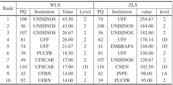
Table 5– The 10 researchers best positioned in the average links strength.
Rank WLS ZLS
PQ Institution Value Level PQ Institution value level
1 108 UNISINOS 43.50 2 74 UFF 254.67 2
2 56 UNISINOS 43.00 2 108 UNISINOS 184.00 2
3 107 UNISINOS 26.67 2 56 UNISINOS 182.00 2
4 81 UFF 26.00 2 62 UFF 178.14 1D
5 74 UFF 21.67 2 41 EMBRAPA 148.00 1D
6 39 PUCPR 18.50 2 81 UFF 130.00 2
7 49 UFSCAR 17.00 2 107 UNISINOS 120.67 2
8 110 UFSCAR 17.00 1D 116 CNEN 102.50 1D
9 42 UFRN 14.00 2 82 INPE 98.00 1A
10 92 UFRN 14.00 2 39 PUCPR 95.00 2
Table 6– Correlations of metrics of the average link strength with the fellowship levels.
Correlations
WLS ZLS
Fellowship Level 0.003 0.131*
*The correlation is significant at the level 0.05 two-tailed test.
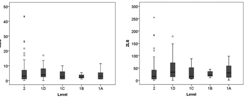
Figure 5 shows the boxplots graphs to evaluate and compare the distributions of averages link strength among the fellowship levels. Level 1D shows the highest variability and highest median in both metrics. Levels 2 and 1D have outliers.
Figure 5– Box plots of the average link strength.
4.4 Closeness Centrality
Table 7 shows the results of the 10 authors better positioned, according to the unweighted close-ness centrality – UCC; W-weighted closeclose-ness centrality – WCC and Z-weighted closeclose-ness cen-trality – ZCC.
Table 7– The 10 researchers best positioned according to closeness centrality.
Rank UCC WCC ZCC
PQ Institution value level PQ Institution value level PQ Institution value level 1 124 UFSCar 0.1834 1A 124 UFSCar 0.3010 1A 124 UFSCar 2.2633 1A
2 32 USP 0.1740 1B 60 USP 0.2915 1A 60 USP 2.2266 1A
3 60 USP 0.1713 1A 112 ITA 0.2838 1B 32 USP 2.1843 1B
4 61 USP 0.1704 2 32 USP 0.2808 1B 112 ITA 2.1621 1B
5 14 ITA 0.1650 1C 33 UFSCar 0.2769 2 33 UFSCar 2.1269 2
6 103 UFMG 0.1618 1C 14 ITA 0.2763 1C 61 USP 2.1004 2
7 47 UNESP/BAU 0.1618 2 61 USP 0.2739 2 103 UFMG 2.0902 1C 8 112 ITA 0.1595 1B 47 UNESP/BAU 0.2681 2 144 UFSCar 2.0877 1D
9 76 USP 0.1595 1B 76 USP 0.2678 1B 36 UFSCar 2.0732 2
To illustrate the change in the positions of the nodes in the three closeness centrality metrics observe researchers PQ32 and PQ60. Researcher PQ32 is the second closest of the other nodes, by UCC, in this case, the sum of the distances from it and the other nodes is smaller than the sum of the distances of PQ60 to other nodes. However, considering WCC, the paths that connect researcher PQ60 to other nodes are formed by more frequent connections than those from the paths that connect researcher PQ32 to other nodes. As the frequency of connections shortens the paths, researcher PQ60 obtained a better position according to WCC. This researcher also remained in second place according to ZCC.
Regarding the fellowship level, researchers with higher levels predominate among the 10 posi-tions according to the three metrics of closeness centrality. Level 2 researchers take on average three positions in this table. Researchers working at USP and UFScar are predominant in these rankings, implying that PQs at these institutions have easier access to other PQs in the network. PQ124 from UFScar obtained the highest value according to the three methods, what shows a proeminent position in the network. Table 8 shows the correlations of the three metrics of close-ness centrality with the fellowship level.
Table 8– Correlations of the closeness centrality metrics with the fellowship levels.
Correlations
UCC WCC ZCC
Level of the fellowship 0.211** 0.182** 0.229**
**The correlation is significant at the level 0.01 two-tailed test.
The three closeness centrality metrics showed significant positive correlations with the fellowship level. The one that presented the highest correlation was ZCC, followed by UCC. Thus, because they have higher possibilities of establishing partnerships publications, researchers with greater closeness centralities also tend to have a higher fellowship level. Furthermore, the researcher who is closest to the leading researchers tends to have a higher fellowship level.
Figure 6 presents the box plots to evaluate and compare the distributions of closeness centralities among the fellowship levels. In the first two graphs, the highest variability is obtained by level 1C, and the highest median and smallest variability are obtained by level 1B. In the third graph, level 2 has the highest variability and level 1B maintains the highest median.
4.5 Betweenness Centrality
Table 9 shows the results of the top 10 authors according to the unweighted betweenness central-ity – UBC; W-weighted betweenness centralcentral-ity – WBC; and Z-weighted betweenness centralcentral-ity – ZBC.
Figure 6– Box plots of the closeness centrality.
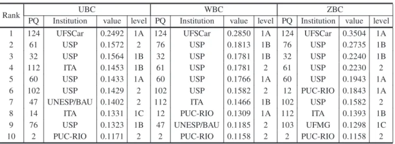
Table 9– The top researchers 10 positioned in the betweenness centrality.
Rank UBC WBC ZBC
PQ Institution value level PQ Institution value level PQ Institution value level 1 124 UFSCar 0.2492 1A 124 UFSCar 0.2850 1A 124 UFSCar 0.3504 1A
2 61 USP 0.1572 2 76 USP 0.1813 1B 76 USP 0.2735 1B
3 32 USP 0.1564 1B 32 USP 0.1781 1B 32 USP 0.2240 1B
4 112 ITA 0.1453 1B 61 USP 0.1781 2 61 USP 0.2230 2
5 60 USP 0.1433 1A 60 USP 0.1766 1A 60 USP 0.1943 1A
6 102 USP 0.1429 2 102 USP 0.1582 2 12 PUC-RIO 0.1843 1A 7 47 UNESP/BAU 0.1402 2 112 ITA 0.1466 1B 102 USP 0.1582 2 8 14 ITA 0.1331 1C 12 PUC-RIO 0.1309 1A 112 ITA 0.1393 1B 9 76 USP 0.1323 1B 47 UNESP/BAU 0.1185 2 103 UFMG 0.1298 1C 10 2 PUC-RIO 0.1171 2 2 PUC-RIO 0.1158 2 2 PUC-RIO 0.1158 2
Table 10– Correlations of the betweenness centrality metrics with the fellowship levels.
Correlations
UBC WBC ZBC
Fellowship Level 0.241** 0.307** 0.367**
**The correlation is significant at the level 0.01 two-tailed test.
The three betweenness centralities metrics showed significant positive correlations with the fel-lowship level. The one that presented the highest correlation with the felfel-lowship level was ZBC, that is, considering the importance of nodes, followed by WBC. Thus, researchers who assume the role of “intermediary”, controlling the frequency of information flow tend to have higher lev-els of productivity, however, those that intermediate nodes in paths whose connections are more frequent and or have the most important nodes have higher fellowship levels.
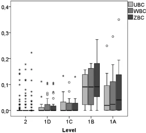
In Figure 7, you can view the center, the dispersion, the diversion of symmetry and the identifi-cation of the observations considered atypical. In these three graphs, levels 1A and 1B show the highest variability and level 1B the highest medians. Level 2 has the smallest variation and the highest number of atypical points.
Figure 7– Box plot of the betweenness centrality.
4.6 Eigenvector Centrality
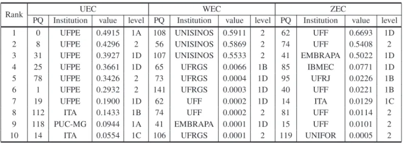
Table 11– The top 10 researchers according to the eigenvector centrality.
Rank UEC WEC ZEC
PQ Institution value level PQ Institution value level PQ Institution value level 1 0 UFPE 0.4915 1A 108 UNISINOS 0.5911 2 62 UFF 0.6693 1D
2 8 UFPE 0.4296 2 56 UNISINOS 0.5869 2 74 UFF 0.5408 2
3 31 UFPE 0.3927 1D 107 UNISINOS 0.5533 2 41 EMBRAPA 0.5022 1D 4 25 UFPE 0.3661 1D 65 UFRGS 0.0066 1B 85 IBMEC 0.0771 1D
5 78 UFPE 0.3426 2 73 UFRGS 0.0004 1D 95 UFRJ 0.0226 1B
6 1 UFPE 0.2932 2 141 UFRGS 0.0003 1D 40 UFF 0.0221 1B
7 19 UFPE 0.1900 1D 62 UFF 0.0002 1D 14 ITA 0.0129 1C
8 112 ITA 0.1433 1B 74 UFF 0.0002 2 81 UFF 0.0114 2
9 118 PUC-MG 0.0944 1A 41 EMBRAPA 0.0001 1D 15 UFF 0.0101 2 10 14 ITA 0.0554 1C 106 UFRGS 0.0001 2 119 UNIFOR 0.0005 2
It is evident that the composition of the top 10 positions according to the three eigenvector cen-trality metrics are formed by different researchers, only researcher PQ14, tenth placed in UEC appears twice in the table position 7 in ZEC. As for researchers fellowship levels, the major-ity are of levels 2 and 1D. UFPE, UNISINOS and UFF have the PQs with highest UEC, WEC and ZEC values, respectively. The correlations among the eigenvector centrality metrics and the fellowship level are presented in Table 12.
Table 12– Correlations of the eigenvector centrality metrics with the fellowship levels.
Correlations
UEC WEC ZEC
Fellowship Level 0.199** 0.154* 0.186**
*The correlation is significant at the level 0.05 two-tailed test.
**The correlation is significant at the level 0.01 two-tailed test.
For the eigenvector centrality, researchers connected with more central researchers in accor-dance with the degree, have higher centrality. Thus, according to UEC, (resp., WEC or ZEC) a researcher will have a higher centrality if he is connected to researchers with greater UEC (resp., WEC or ZEC). The correlations of these metrics with the fellowship level were significant, es-pecially UEC and ZEC.
Figure 8 presents the box plots to evaluate and compare the distributions of the eigenvector centralities among the fellowship levels. To get a better view were disregarded in these graphs the isolated nodes they have eigenvector centrality equal to zero and the scale used was logarithmic. You can view that level 1A has the greatest variability.
4.7 PageRank
Figure 8– Box plots of the eigenvector centrality.
the ranking of the researchers according to these three metrics remain almost unchanged. PQ124 and PQ82 have obtained the highest values for the PageRank, implying that their importance in the network is related to having collaborated with other proeminent PQs.
Table 13– The top 10 researchers according to the PageRank.
Rank UPR WPR ZPR
PQ Institution value level PQ Institution value level PQ Institution value level 1 124 UFSCar 0.026 1A 82 INPE 0.025 1A 124 UFSCar 0.032 1A 2 84 PUC-RIO 0.018 1D 124 UFSCar 0.024 1A 82 INPE 0.026 1A
3 114 UFSC 0.017 1C 0 UFPE 0.021 1A 0 UFPE 0.025 1A
4 62 UFF 0.016 1D 62 UFF 0.021 1D 62 UFF 0.025 1D
5 65 URGS 0.016 1B 12 PUC-RIO 0.019 1A 12 PUC-RIO 0.024 1A
6 0 UFPE 0.015 1A 9 UNIFEI 0.019 2 111 UFRJ 0.022 1A
7 111 UFRJ 0.014 1A 111 UFRJ 0.018 1A 9 UNIFEI 0.019 2
8 9 UNIFEI 0.014 2 117 UNIFEI 0.017 1D 117 UNIFEI 0.018 1D
9 82 INPE 0.013 1A 114 UFSC 0.015 1C 114 UFSC 0.016 1C
10 85 IBMEC 0.013 1D 102 USP 0.014 2 41 EMBRAPA 0.015 1D
Table 14 shows that the correlations of the PageRank with the fellowship level are significant. However, the UPR value of the researcher has the greatest impact on the fellowship level.
Table 14– Correlations of PageRank with the fellowship levels.
Correlations
UPR WPR ZPR
Fellowship Level 0.240** 0.160* 0.211**
*The correlation is significant at the level 0.05 two-tailed test.
**The correlation is significant at the level 0.01 two-tailed test.
Figure 9– Box plots of the PageRank.
4.8 Local clustering coefficient
Table 15 presents the rankings of the top 10 researchers according to the unweighted local clus-tering coefficient – ULC; W-weighted local clusclus-tering coefficient – WLC and; Z-weighted local clustering coefficient – ZLC. The composition of this table is formed basically by level 2 re-searchers. And their positions according to the three metrics are almost the same.
The clustering coefficient of a given researcher indicates how many collaborators are collabo-rating with each other. However, these metrics have no impact on the fellowship level of the researcher, as indicate correlations in Table 16. High clustering coefficient may imply that the researcher does not have a very diverse group of collaborators. UFPE, UFRJ and UTFPR have the higher number of PQs among the 27 greater values of ULC, while UNISNOS and UTFPR have PQs with high WLC and ZLC values.
Table 15– The top 10 researchers according to the Local Clustering Coefficient.
Rank ULC WLC ZLC
PQ Institution value level PQ Institution value level PQ Institution value level
1 56 CNEN 1.00 2 56 UNISINOS 0.89 2 56 UNISINOS 0.31 2
2 108 UFPE 1.00 2 108 UNISINOS 0.89 2 108 UNISINOS 0.31 2
3 74 UFPE 1.00 2 134 UNIFEI 0.31 2 74 UFF 0.28 2
4 134 UFPE 1.00 2 74 UFF 0.31 2 134 UNIFEI 0.14 2
5 33 UFRJ 1.00 2 107 UNISINOS 0.29 2 107 UNISINOS 0.10 2 6 137 UFRJ 1.00 1D 137 PUCRIO 0.15 1D 41 EMBRAPA 0.10 1D
7 50 UTFPR 1.00 2 50 UTFPR 0.14 2 95 UFRJ 0.09 1B
8 70 UTFPR 1.00 2 70 UTFPR 0.14 2 50 UTFPR 0.08 2
9 77 UTFPR 1.00 1C 77 UTFPR 0.14 1C 70 UTFPR 0.08 2
10 66 UFF 1.00 2 54 UFES 0.13 2 77 UTFPR 0.08 1C
Note: Other 17 researchers have ULC equal to 1.
Table 16– Correlations of the Local Clustering Coefficient with the fellowship levels.
Correlations
ULC WLC ZLC
Fellowship Level 0.043 0.029 0.044
4.9 Eccentricity
Table 17 displays the 10 researchers with lowest eccentricities values, which corespond to the most central ones. These values were obtained from three distinct forms: unweighted eccentricity – UE; W-weighted eccentricity – WE; Z-weighted eccentricity – ZE. Researchers of different levels are listed in this table. These are the researchers with the smallest maximum distances from them to any other in the giant component of the network. Many of the researchers in the top-10 positions of UE do not figure in the top-10 according to WE or ZE. In fact, as the weights of the edges and the weights of the edges combined with the nodes’ attributes shorten the paths, other researchers were prioritized. Among the institutions are frequent UNESP-BAU, UFSCar and USP.
Table 17– The 10 researchers best positioned in eccentricity.
Rank UE WE ZE
PQ Intitution value level PQ Intitution value level PQ Institution value level
1 47 UNESP/BAU 7 2 32 USP 4.67 1B 61 USP 0.70 2
2 124 UFSCar 7 1A 61 USP 4.97 2 76 USP 0.78 1B
3 14 ITA 8 1C 47 UNESP/BAU 5.32 2 12 PUC-RIO 0.78 1A
4 23 USP 8 2 76 USP 5.45 1B 102 USP 0.80 2
5 32 USP 8 1B 14 ITA 5.47 1C 86 UNESP/BAU 0.80 2
6 33 UFSCar 8 2 102 USP 5.62 2 104 IBGE 0.81 2
7 36 UFSCar 8 2 124 UFSCar 5.67 1A 32 USP 0.82 1B
8 60 USP 8 1A 12 PUC-RIO 5.70 1A 45 PUC-RIO 0.82 1C
9 61 USP 8 2 48 USP 5.72 2 48 USP 0.82 2
10 86 UNESP/BAU 8 2 86 UNESP/BAU 5.76 2 114 UFSC 0.84 1C
Note: The researchers PQ97 UNESP/BAU level 2, PQ103 UFMG level 1C, PQ105 UNESP/BAU level 2,
PQ115 UNESP/BAU level 1A, PQ136 UNESP/BAU level 2 and PQ144 UFSCar level 1D also have UE equal 8.
The relationship of a researcher with other researchers is better the smaller the eccentricity is. However, none of the metrics of eccentricity significantly impacts the fellowship level, as shown in the Table 18.
Table 18– Correlations of the eccentricity with the fellowship levels.
Correlations
UE WE ZE
Fellowship Level –0.139 –0.052 –0.121
Figure 11– Box plots of the eccentricity.
4.10 Utility
The top 10 reasearchers acccording to their utility or benefit of belonging to network structure is shown in Table 19. The utility was obtained in three different ways: unweighted utility – UU; W-weighted utility – WU; and Z-weighted utility – ZU. The researchers from lower levels 2 and 1D are the ones that have the greatest benefits in UU, and the level 1A researchers occupy 50% the 10 top positions according to WU and ZU. All researchers in the WU list also appear in the ZU list. Once more PQ124 has a proeminent posisiton in the rankings according to all methods.
The benefit of a researcher belonging to the network impacts significantly and in a moderate way his fellowship level, as shown in Table 20. The highest correlation is obtained with ZU followed by UU.
Table 19– The 10 researchers best positioned according to the utility.
Rank UU WU ZU
PQ Intitution value level PQ Intitution value level PQ Institution value level 1 124 UFSCar 6.32 1A 124 UFSCar 6.12 1A 124 UFSCar 7.49 1A
2 114 UFSC 5.50 1C 82 INPE 5.43 1A 0 UFPE 6.32 1A
3 85 IBMEC 4.21 1D 114 UFSC 5.43 1C 82 INPE 6.01 1A
4 9 UNIFEI 4.10 2 0 UFPE 5.00 1A 114 UFSC 5.64 1C
5 143 UFRJ 4.00 2 9 UNIFEI 4.80 2 111 UFRJ 5.44 1A
6 84 PUC-RIO 3.96 1D 111 UFRJ 4.34 1A 12 PUC-RIO 4.86 1A
7 62 UFF 3.65 1D 12 PUC-RIO 4.11 1A 9 UNIFEI 4.78 2
8 82 INPE 3.64 1A 143 UFRJ 4.00 2 62 UFF 4.63 1D
9 52 USP 3.44 1C 62 UFF 3.98 1D 143 UFRJ 4.00 2
10 65 UFRJ 3.43 1B 135 PUC-PR 3.97 2 135 PUC-PR 3.97 2
Table 20– Correlations of the utility with the fellowship levels.
Correlations
UU WU ZU
Fellowship Level 0.251** 0.228** 0.257**
**The correlation is significant at the level 0.01 two-tailed test.
Figure 12– Box plots of the utility.
4.11 Logistic regression
variables, For that, we use a multivariate logisitc regression analysis, where SNA metrics are in-dependent variables and the level of the research productivity grant is the in-dependent value. Since we do not have many researchers in each level 1 fellowship, we grouped all level 1 fellowships in a single group (1) and level 2 felloships received value 0. In this analysis, we consider only the researchers that belong to the main component of the network, since the values of some metrics for nodes in different components may not be comparable.
The first model, a logistic regression analysis was performed to determine the effects of un-weighted metrics (U) on the fellowship level of researchers. The metrics considered in this re-gression were: E-I indexl, E-I indexr , UDC, UCC, UBC, UEC, ULC, UE and UU. The UPR was excluded to avoid the effect of multicollinearity. The logistic regression model was statis-tically significant,χ2 = 37.859, p < 0.0005. The model explained 45.30% (Nagelkerke R2) of the variation of the fellowship level and correctly classified 77.17% of the cases. Of the nine predictors, only two are statistically significant, the result is shown in the Table 21. Thus, we con-clude that the unweighted metrics (E-I indexl and Utility) positively influence the researchers’ fellowships level.
Table 21– Model summary.
Estimation Standard error Wald p-value
Intercept –0.898 0.345 6.779 0.009
E-I indexl 1.788 0.445 16.120 0.000
UU 1.244 0.390 10.166 0.001
The second model, we used the logistic regression was performed to determine the effects of weighted metrics (W) on the fellowships level of researchers. The metrics considered in this regression were: E-I indexl W, E-I indexr, WDC, WCC, WBC, WEC, WLC, WE, WU and WLS. The WPR was excluded to avoid the effect of multicollinearity. The logistic regression model was statistically significant,χ2 = 32.543, p < 0.0005. The model explained 39,78% (Nagelkerke R2) of the variation of the level of productivity and correctly classified 75.00% of the cases. Of the ten predictor variables four are statistically significant, the result is shown in the Table 22 below. According to the result, we conclude that the metrics weighted (E-I indexl, Betweenness centrality, Utility and Eccentricity) positively influence the researchers’ fellowships level.
Table 22– Model summary.
Estimation Standard error Wald p-value
Intercept –0.749 0.302 6.131 0.013
E-I indexl W 1.246 0.339 13.509 0.000
WBC 0.803 0.349 5.302 0.021
WU 0.618 0.309 3.997 0.046
In the third model, the effects of the weighted metrics with the insertion of the nodes’ attributes (Z) on the fellowship level of researchers were also analyzed by a logistic regression analysis. The metrics considered in this regression were: E-I indexl Z, E-I indexr Z, ZCC, ZBC, ZEC, ZLC, ZE, ZU and ZLS. The ZDC and ZPR were excluded to avoid the effect of multicollinearity. The logistic regression model was statistically significant,χ2=35.182,p<0.0005. The model explained 42.43% (Nagelkerke R2) of the variation of the level of productivity and correctly classified 77.2% of the cases. Of the nine predictor variables five are statistically significant, the result is summarized in the Table 23 below. We find that the weighted metrics with the insertion of the nodes’ attributes (E-I indexl Z, Betweenness centrality, Eigenvector centrality, Utility and Average of the strong links) act positively in the researchers’ fellowships level.
Table 23– Model summary.
Estimation Standard error Wald p-value
Intercept –0.609 0.309 3.888 0.049
E-I indexl Z 1.248 0.387 10.374 0.001
ZBC 0.564 0.297 3.602 0.058
ZEC 0.705 0.393 3.213 0.073
ZU 1.070 0.412 6.736 0.009
ZLS –0.871 0.499 3.046 0.081
Comparing the three models, we see that there is evidence that SNA metrics involving the weight of edges and the authors’ attributes contextualize with more information (resources) ways a re-searcher can achieve better productivity. Moreover, the E-I indexl and Utility have shown to be in all models the metric which most influenced the fellowships level, they are present in the three models. Thus, researchers which are to collaborate with other researchers who devote most of their attention to their mutual project are more likely to hold a level 1 fellowship. As well as seek partnerships with researchers from different fellowship levels. The betweenness centrality also has a positive participation in the definition of scholarship levels, but only in the second and third models, so researchers who assume the role of “intermediary”, in paths whose connections are more frequent and have the most important nodes, tend to have level 1 fellowship.
Souza et al. (2016) also developed a logistic regression model to verify the influences of the un-weighted metrics (Degree Centrality, Betweenness Centrality, Closeness Centrality, Eigenvector Centrality, Eccentricity, Cluster Coefficient and Utility) in the fellowships level of researchers in the Probability and Statistic area. And as a result, the degree centrality had a positive effect and the average distance (which was defined as closeness centrality in Souza et al. (2016)) had a negative effect on the fellowship level.
5 CONCLUSIONS
Such metrics were divided among unweighted, weighted by edges, and weighted by edges and nodes. The metrics analyzed were: theE-Iindex, the Degree centrality, the Average link strength, the Closeness centrality, the Betweenness centrality, the Eigenvector centrality, the PageRank, the Eccentricity, the Local clustering coefficient and the Utility.
The unweighted metrics that showed the greatest association with the fellowship level were: the E-Iindexl 0.406, the utility 0.251, the degree centrality 0.244, the betweenness centrality 0,241 and the PageRank 0.240. The metrics weighted by edges which presented the highest association with the fellowship level were: the betweenness centrality 0.307, theE-Iindexl 0.343 and the utility 0.228. The metrics weighted by edges and nodes which presented highest association with the fellowship level were: the betweenness centrality 0.367, theE-Iindexl0.302, the utility 0.257
and the closeness centrality 0.229.
Thus, the major conclusions of this paper are:
• As compared to the co-authorship network of PQs in the Probability and Statistic area, although the Industrial Engineering community is larger, the collaboration among the PQs is not as strong;
• The E-I indexl analysis shows that the geographical distances is still a main barrier to collaboration among PQs in the Industrial Engineering community;
• researchers who assume a role of mediator (greater betweenness centralities) controlling the flow of information, tend to have higher fellowship levels, especially those among the nodes whose paths are formed by connections more frequent or feature more important researchers;
• researchers of higher ranking, by the unweighted PageRank, also have higher fellowship levels. If the PageRank is weighted by edges and nodes, the impact on the fellowship level is lower;
• researchers who present the highest unweighted degree centralities, namely, greater numbers of co-authors, tend to have higher fellowship levels. If the degree centrality is weighted this trend decreases;
• researchers who present greater possibilities for establishing publications partnerships are those with greater closeness centralities and with higher fellowship levels, especially if the partners are researchers with the highesth-index;
• researchers with greater benefits of belonging the network (greater Utility) also have the highest fellowship levels, especially those that have highh-index or collaborate with re-searchers with the highesth-index;
• UNISINOS, UFF, USP, UFScar, UFPE and UTFPR are the institutions that hold the higher number of PQs among the top 10 according to some SNA metrics;
• PQ124, from UFScar, was the one more important in the network according to a greater number of metrics.
• Finally, through a logistic regression analysis, the unique metrics that, according to all three methods, influence the fellowship level being of level 1 as opposed to level 2 are the E-I indexl and the Utility. This implies that level 2 PQs desiring to obtain a level 1 fellowship should both collaborate with level 1 PQs and also concentrate collaboration with other PQs that devote much of their collaboration effort in their relationship.
It is important to note that fellowships are granted for a period of time ranging from 3 years (level 2) up to 5 years (level 1A). Thus, researchers only compete with those that are in the same time cycle, what can cause some discrepancies between different cycles. However, on August 2013, all fellowship levels were reclassified, Figueiredo (2013), to reduce those discrepancies. Since our data was collected on March 2014, this problem of the time cycle was mitigated.
It is worth mentioning that the network was formed only among researchers with CNPq grant in research productivity in the area of Industrial Engineering in Brazil. Thus, in this network, it was not considered the co-authorship relations between them and other non-fellows authors or of other PQs in different areas of knowledge. For future work, one can develop a network that involves beyond the relations among the fellows, their other relationships. And compare the results of the correlations of the network metrics with those studied in this work. Other types of weights of the authors, besides theh-index, may also be studied to evaluate how that would change the results shown here.
REFERENCES
[1] ABBASIA & ALTMANNJ. 2011. “On the correlation between research performance and social net-work analysis measures applied to research collaboration netnet-works”. In: Hawaii International Con-ference on System Sciences, Proceedings of the 41st Annual. Waikoloa, HI: IEEE.
[2] ABBASIA, ALTMANNJ & HOSSAINL. 2011. Identifying the effects of co-authorship networks on the performance of scholars: A correlation and regression analysis of performance measures and social network analysis measures.Journal of Informetrics,5: 94–607.
[3] ABBASIA, HOSSAINAL & LEYDESDORFFL. 2012. Betweenness centrality as a driver of pref-erential attachment in the evolution of research collaboration networks.Journal of Informetrics,6: 403–412.
[4] ANASTASIOST, SGOIROPOULOUC, PAPAGEORGIOUE, TERRAZO & MIAOULIS, G. 2012. Co-authorship networks in academic research communities: the role of network strength. 16th Panhel-lenic Conference on Informatics.
[6] ANDRADERL & R ˆEGOLC. 2015a. Conhecendo a rede de coautoria dos bolsistas de produtividade em pesquisa da ´area de engenharia de produc¸˜ao e a sua influˆencia no n´ıvel de produtividade. In: XLVII Simp´osio Brasileiro de Pesquisa Operacional – SBPO.
[7] ANDRADERL & R ˆEGOLC. 2015b. A influˆencia da rede de coautoria no n´ıvel das bolsas de pro-dutividade da ´area de engenharia de produc¸˜ao. In: XXXV Congresso da Sociedade Brasileira de Computac¸˜ao – CSBC.
[8] BARNETT AH, AULT RW & KASERMANDL. 1988. The Rising Incidence of Co-authorship in Economics: Further Evidence.Review of Economics and Statistics,70: 539–543.
[9] BONACICHP. 1987. Power and centrality: a family of measures.The American Journal of Sociology, 92: 1170–1182.
[10] CN. 2015. Crit´erios de Julgamento. Available in: <http://www.cn.br/web/guest/criterios-de-julga-mento>. Access em: 28 de janeiro de 2015.
[11] EATON JP, WARD JC & KUMARA. 1999. Structural Analysis of Co-Author Relationships and Author Productivity in Selected Outlets for Consumer Behavior Research.Journal of Consumer Psy-chology,8: 39–59.
[12] EGGHEL. 2006. Theory and practise of theg-index.Scientometrics,69: 131–152.
[13] FIGUEIREDORWDE. 2013. CNPq reclassifica pesquisadores e 39 docentes da UFC s˜ao promovidos. Available in: <http://www.ufc.br/noticias/noticias-de-2013/4013-cnpq-reclassifica-pesquisadores-e-39-docentes-da-ufc-sao-promovidos>. Access on: 30 May 2017.
[14] FREEMANLC. 1979. Centrality in Social Networks Conceptual Clarification.Social Networks,1: 215–239.
[15] HAIRJF, BLACKWC, BABINBJ, ANDERSONRE & TATHAMRL. 2009. An´alise multivariada de dados. Bookman Editora.
[16] HANNEMANRA & RIDDLEM. 2005. Introduction to social network methods. Riverside: University of Calif´ornia.
[17] HIRSCHJE. 2005. An index to quantify an individual’s scientific research output.Proceedings of the National Academy of Sciences,102: 16569–16572.
[18] HUANGP-Y, LIUH-Y, CHENC-H & CHENGP-J. 2013. The impact of social diversity and dynamic influence propagation for identifying influencers in social networks, in: Web Intelligence WI and Intelligent Agent Technologies IAT, 2013 IEEE/WIC/ACM International Joint Conferences on, vol. 1, p. 410–416.
[19] HUDSONJ. 1996. Trends in Multi-Authored Papers in Economics.Journal of Economic Perspectives, 10: 153–158.
[20] JACKSONMO. 2008. Social and Economic Networks. Princeton University Press. Stanford Univer-sity, February 2008.
[21] JACKSONMO & WOLINSKYA. 1996. A Strategic Model of Social and Economic Networks.Journal of economic theory,71: 44–74.
[23] KRACKHARDTD & STERNR. 1988. Informal networks and organizational crises: An experimental simulation.Social Psychology Quarterly,51: 123–140.
[24] KRACKHARDTD. 1992. The strength of strong ties: The importance of philos in organizations. In Networks and Organizations: Structure, Form, and Action, p. 216–239.
[25] LEES & BOZEMANB. 2005. The impact of research collaboration on scientific productivity.Social Studies of Science,35: 673–702.
[26] LIUJ, LIY, RUANZ, FUG, CHENX, SADIQR & DENGY. 2014. A new method to construc to co-author networks.Physica A,419: 29–39.
[27] LIUX, BOLLENJ, NELSONML & SOMPELHVAN DE. 2005. Co-authorship networks in the digital library research community.Information Processing and Management,41: 1461–1480.
[28] MENA-CHALCOJP & CESARJRRM. 2009. ScriptLattes: An open-source knowledge extraction system from the Latts platform.Journal of the Braszilian Computer Society,15: 31–39.
[29] NEWMANMEJ. 2001a. The structure of scientific collaboration networks.Proceeding of the National Academy of Sciences,98: 404–409.
[30] NEWMANMEJ. 2001b. Scientific collaboration networks. I. Network constructions and fundamental results.Physical Review E, vol. 64.
[31] NEWMAN MEJ. 2001c. Who is the best connected scientist? A study of scientific coauthorship networks.Complex Networks,650: 337–370.
[32] NEWMANMEJ. 2004. Coauthorship networks and patterns of scientific collaboration.Proceeding of the National Academy of Sciences,101: 5200–5204.
[33] ONEL S, ZEIDA & KAMARTHIS. 2011. The structure and analysis of nanotechnology co-author and citation networks.Scientometrics,89: 119–138.
[34] ONNELA J-P, SARAMAKI¨ J, KERTESZ´ J & KASKIK. 2015. Intensity and coherence of motifs in weighted complex networks.Physical Review E,716: 4.
[35] SANTOSAMDOS. 2014. Aplicac¸˜oes de modelos de grafos na an´alise de conceitos e de redes sociais. Recife. 2014. 162 p. Doutorado – Programa de P´os-graduac¸˜ao em Estat´ıstica/UFPE.
[36] SOUZAFC DE, AMORIMRM & R ˆEGOLC. 2016. A Co-authorship network analysis of CNPq’s productivity research fellows in the probability and statistic area.Perspectivas em Ciˆencia da Infor-mac¸ ˜ao,21(4), 29–47.
[37] WANDERLEYAJ, DUARTEAN, BRITOAVDE, PRESTESMAS & FRAGOSOFC. 2014. Identifi-cando correlac¸ ˜oes entre m´etricas de An´alise de Redes Sociais e oh-index de pesquisadores de Ciˆencia da Computac¸˜ao. In. XXXIV Congresso da Sociedade Brasileira de Computac¸˜ao – CSBC, 2014.
[38] WAINERJ & VIEIRAP. 2013. Correlation between bibliometrics and peer evaluation for all disci-plines: the avaluation of Brazilian scientists.Scientometrics online,96: 395–410.
[39] WASSERMANS & FAUSTK. 1994. Social Networks Analysis: Methods and Applications. Cam-bridge University Press.Structural analysis in social the social sciences series, vol. 8.
[40] YANE & DINGY. 2009. Applying centrality measures to impact analysis: A coauthorship network